Learning Invariant Features Using Inertial Priors Thomas Dean Department of Computer Science Brown University Providence, Rhode Island 02912 CS-06-14 November 2006

Learning Invariant Features Using Inertial Priors∗ Thomas Dean Department of Computer Science Brown University, Providence, RI 02912 November 30, 2006

Abstract We address the technical challenges involved in combining key features from several theories of the visual cortex in a single coherent model. The resulting model is a hierarchical Bayesian network factored into modular component networks embedding variable-order Markov models. Each component network has an associated receptive field corresponding to components residing in the level directly below it in the hierarchy. The variable-order Markov models account for features that are invariant to naturally occurring transformations in their inputs. These invariant features give rise to increasingly stable, persistent representations as we ascend the hierarchy. The receptive fields of proximate components on the same level overlap to restore selectivity that might otherwise be lost to invariance. Keywords: graphical models, machine learning, Bayesian networks, neural modeling

1

Introduction

Supervised learning with a sufficient number of correctly labeled training examples is reasonably well understood, and computationally tractable for a restricted class of models. In particular, learning simple concepts, e.g., conjunctions, from labeled data is computationally tractable [62]. For applications in machine vision, however, labeled data is often scarce and the concepts we hope to learn are anything but simple. Moreover, adult humans have little trouble acquiring new concepts with far fewer examples than computational learning theory might suggest. It would seem that we rely on a large set of subconcepts acquired over a lifetime of training to quickly acquire new concepts [45, 33]. Our visual memory apparently consists of many simple features arranged in layers so that they build upon one another to produce a hierarchy of representations [22, 55]. We posit that learning such a hierarchical representation from examples (input and and output pairs) is at least as hard as learning polynomial-size circuits in which the subconcepts are represented as bounded-input boolean functions. Kearns and Valiant showed that the problem of learning polynomial-size circuits (in Valiant’s probably approximately correct learning model) is infeasible given certain plausible cryptographic limitations [37]. However, if we are provided access to the inputs and outputs of the circuit’s internal subconcepts, then the problem becomes tractable [56]. This implies that if we had the “circuit diagram” for the visual cortex and could obtain labeled data, inputs and outputs, for each component feature, robust machine vision might become feasible. There are many researchers who believe that detailed knowledge of neural circuitry is not needed to solve the vision problem. Numerous proposals suggest plausible architectures for sufficiently powerful hierarchical ∗

A slightly amended version of this technical report will appear in the Annals of Mathematics and Artificial Intelligence.

1

models [28, 44]. Assuming we adopt one such proposal, we are still left with the problem of acquiring training data to learn the component features. The most common type of cell in the visual cortex, called a complex cell by Hubel and Wiesel [32, 31], is capable of learning features that are invariant with respect to transformations of its set of inputs or receptive field. Consider, for example, a cell that responds to a horizontal bar no matter where the bar appears vertically in its receptive field. F¨oldi´ak [19], Wiskott and Sejnowski [65], Hawkins [24] and others suggest that we can learn a hierarchy of such features by exploiting the property that the features we wish to learn change gradually while the transformed inputs change quickly. To understand the implications of this viewpoint for learning, it is as though we are told that consecutive inputs in a time series, e.g., the frames in a video sequence, are likely to have the same label. We are not explicitly provided a label, but knowing that frames with the same label tend to occur consecutively is a powerful clue to learning naturally occurring variation within a concept class. In this paper, we develop a probabilistic model of the visual cortex capable of learning a hierarchy of invariant features. The resulting computational model takes the form of a Bayesian network [53, 35, 34] which is constructed from many smaller networks each capable of learning an invariant feature. The primary contribution of this paper is the parameterization and structure of the component networks along with associated algorithms for learning and inference. Since our model builds upon ideas from several theories of the visual cortex, we begin with a discussion of those ideas and how they apply to our work.

2

Computational Models of the Visual Cortex

In this paper, we make use of the following key ideas in developing a computational model of the visual cortex. Subsequent sections explore in detail how each of these ideas is applied in our model. • Lee and Mumford [42] propose a model of the visual cortex as a hierarchical Bayesian network in which recurrent feedforward and feedback loops serve to integrate top-down contextual priors and bottom-up observations. • Fukushima [22] and F¨oldi´ak [19] suggest that units within each level of the hierarchy form composite features from the conjunction of simpler features at lower levels to achieve shift- and scale-invariant pattern recognition.1 • Ullman and Soloviev [61] describe a model in which overlapping receptive fields are used to deal with the problem of false conjunctions which arises when invariant features are combined without consideration of their relationships. • F¨oldi´ak [19], Wiskott and Sejnowski [65] and Hawkins and George [25] propose learning invariances from temporal input sequences by exploiting the observation that sensory input tends to vary quickly while the environment we wish to model changes gradually. Borrowing from Lee and Mumford, we start with a hierarchical Bayesian network to represent the dependencies among different cortical areas and employ particle filtering and belief propagation to model the interactions between adjacent levels in the hierarchy. This approach presents algorithmic challenges in terms of performing inference in networks on a cortical scale. To address these challenges, we decompose large networks into many smaller component networks and introduce a protocol for propagating probabilistic constraints that has proved effective in simulation. Following Fukushima and F¨oldi´ak, each component network 1

In order to reliably identify objects invariant with respect to a class of transformations, F¨oldi´ak assumes that the network is trained on temporal sequences of object images undergoing these transformations.

2

implements a feature that abstracts the output of a set of simpler components at the next lower level in the hierarchy. Generalization and invariance according to Ullman and Soloviev arise “not from mastering abstract rules or applying internal transformations, but from using the collective power of multiple specific examples that overlap with the novel stimuli.” Ullman and Soloviev essentially memorize fragments of images and their compositional abstractions and then recombine them to deal with novel images. Their approach to modeling invariants contrasts with approaches that rely on normalizing the input image [51]. The emphasis in the Ullman and Soloviev model is on spatial grouping and neglects the role of time [38]. The observation that the stream of sensory input characterizing our visual experience consists of relatively homogeneous segments provides the key to organizing the large set of examples we are exposed to. Berkes and Wiskott [5] exploit this property to learn features whose output is invariant to transformations in the input by minimizing the first-order derivative of the output. George and Hawkins offer an alternative by memorizing frequently occurring prototypical input sequences which they characterize as having been produced by a common cause, and then classifying novel sequences using Hamming distance to find the closest prototype. In our framework, each component network models the dynamics of the features in the level below, while producing its own sequence of outputs which, combined with the output of proximate features on the same level, produce a new set of dynamic behaviors. The dynamics exhibited by any collection of features need not be Markov of any fixed order, and so we implement our component networks as embedded variable-order Markov models [57] whose variable-duration states serve the same role as George and Hawkins’ prototypical sequences. The network as a whole can be characterized as a spatially-extended hierarchical hidden Markov model [18].

3

Hierarchical Graphical Models

Lee and Mumford model the regions of the visual cortex as a hierarchical Bayesian network. Let x1 , x2 , x3 and x4 represent the first four cortical areas (V1, V2, V4, IT) in the visual pathway and x0 the observed data (input). Using the chain rule and the simplifying assumption that in the sequence hx0 , x1 , x2 , x3 , x4 i each variable is independent of the other variables given its immediate neighbors in the sequence, we write the equation relating the four regions as P (x0 , x1 , x2 , x3 , x4 ) = P (x0 |x1 )P (x1 |x2 )P (x2 |x3 )P (x3 |x4 )P (x4 ) resulting in a graphical model or Bayesian network based on the chain of variables: x0 ← x1 ← x2 ← x3 ← x4 In the Lee and Mumford model, activity in the ith region is influenced by bottom-up feed-forward data xi−1 and top-down probabilistic priors representing feedback from region i + 1: x0

x1

x2

?

x3 -

?

?

P (x0 |x1 )P (x1 |x2 )/Z1

P (x1 |x2 )P (x2 |x3 )/Z2

P (x2 |x3 )P (x3 |x4 )/Z3

6

6

6

φ(x1 , x2 )

φ(x2 , x3 )

φ(x3 , x4 )

where Zi is the partition function associated with the ith region and φ(xi , xi+1 ) is a potential function representing the priors obtained from region i + 1, 3

(a)

(b)

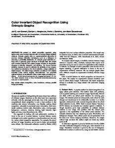
Figure 1: The simple three-level hierarchical Bayesian network (a) employed as a running example in the text is shown along with an iconic rendering of a larger three-dimensional network (b) — two spatial dimensions plus abstraction — using pyramids to depict the component subnetworks. To provide more representational detail in modeling cortical areas, we begin with a graphical model consisting of nodes arranged in K levels. Each directed inter-level edge connects a node in level k to a node in level k − 1. There are also intra-level edges, but, as we will see, these edges are learned and, hence, not present in the graph initially. In general, each level can have more or fewer nodes than the level below it in the hierarchy. However, to illustrate the concepts in our model, we refer to the simple, three-level, hierarchical graphical model shown in Figure 1.a. The term subnet refers to a set of nodes considered together for purposes of decentralized inference. The nodes associated with a particular subnet consist of one node in level k, plus one or more of this node’s children in level k − 1. For reasons that will become apparent in the next section, the node in level k is called the subnet’s hidden node, and the subnet is said to belong to level k. The set of the hidden node’s children in level k − 1 is called the subnet’s receptive field. All of the nodes in the network except those in the input level (k = 1) are discrete, nominal-valued latent variables. The receptive fields for different subnets can overlap, but each node (with the exception of nodes in the input level) is the hidden node for exactly one subnet. The node labeled x1 in Figure 1.a is the hidden node for the subnet with receptive field {y1 , y2 , y3 }. Since we are interested in modeling the visual cortex, receptive fields extend in two spatial dimensions, and so we depict each subnet as a three-dimensional pyramid (two spatial dimensions plus abstraction in the hierarchy of features), and the entire model as a hierarchy of pyramids as illustrated in Figure 1.b. Assuming that each node recursively spans the spatial extent of the nodes in its receptive field, subnets tend to capture increasingly abstract, spatially diffuse features as we ascend the hierarchy. All nodes have roughly the same degree, but the length of edges increases with the level, assuming the obvious threedimensional embedding (see Figure 1.b) and in keeping with the anatomical observations of Braitenberg and Schuz [7]. This property (illustrated in Figure 2) implies that the diameter (the number of edges in the longest shortest path linking any two nodes in a graph) of the subgraph spanning any two adjacent levels in the hierarchy decreases as we ascend the hierarchy. The basic responsibility of a subnet is to implement a discrete-valued feature that accounts for the variance observed in the nodes comprising its receptive field. If we assume variables z1 , ..., z5 are for input only, then there are four subnets shown in Figure 1.a. Now suppose we expand the model in Figure 1 to form a subnet graph as depicted in Figure 3. There is an edge between two subnets in the subnet graph if they share one or more variables. The nodes that comprise a subnet constitute a local graphical model implementing the feature associated with the subnet. The edges in this local graphical model include those connecting the hidden node to the nodes in its receptive field plus additional edges (some of which are learned) as described in the next section.

4

Figure 2: As we ascend the hierarchy, the in- and out-degree of nodes remain constant while the average length of the intra-level edges in the Cartesian embedding of the graph increases, and the diameter of subgraphs spanning adjacent levels decreases.

Figure 3: The hierarchical network from Figure 1.a is expanded to form a graph of subnets. The internal state of each subnet is summarized by a local belief function [53] that assigns a marginal distribution P (x|ξ) to each variable x where ξ signifies evidence in the form of assignments to variables in the input level. The output of a feature is a distribution over the associated subnet’s hidden node assigned by the belief function. The input of a feature corresponds to the vector of outputs of the features associated with its receptive-field variables. In the simplest implementation of our model, every subnet updates its local belief function during each primitive compute cycle. Inference is carried out on the subnet graph in two passes using a variant of generalized belief propagation in which the subnet graph doubles as a region graph [66]. In each complete input cycle, evidence is assigned to the nodes in the input level, and potentials are propagated up the hierarchy starting from the input level and back down starting from the top. Each complete input cycle requires twice the number of primitive compute cycles as there are levels in the hierarchy. If there is no overlap among receptive fields and no intra-level edges, this two-pass algorithm is exact, and a single pass is sufficient for exact inference. If these two conditions are not met, the algorithm is

5

Figure 4: On the left (a) is a depiction of the first two levels in a hierarchy of spatiotemporal abstractions. Spatial variables are projected onto horizontal rows and time extends in the direction of the vanishing point. The nine variables in the first level enclosed in a rectangle identify the spatiotemporal receptive field of one variable in the second level. The graphic on the right (b) illustrates the three stages of spatiotemporal pooling: (1) spatial abstraction, (2) temporal modeling and (3) spatiotemporal aggregation. approximate, but it produces reasonably good approximations when tested against an exact algorithm on small networks (see Murphy et al [47] and Elidan et al [14] for related studies). We limit the propagation of potentials between subnets on the same level; subnets whose receptive fields do overlap participate in a limited exchange of potentials described in Section 7. If two variables on the same level are dependent and the receptive fields for their respective subnets do not overlap, their dependence must be realized primarily though paths ascending and descending the hierarchy.

4

Embedded Hidden Markov Models

Temporal contiguity is at least as important as spatial contiguity in making sense of the world around us. Gestalt psychologists refer to the notion of grouping by common fate, in which elements are first grouped by spatial proximity, and then they are separated from the background when they move in a similar direction [64]. Research on shape from motion attempts to reconstruct the three-dimensional shape of objects from sequences of images by exploiting the short baseline between the consecutive frames of the image sequence [60]. While there are areas of the cortex (the lateral occipital complex) that appear to be specialized for processing shape — relating primarily to spatial contiguity — and areas (the medial temporal and adjacent motion-selective cortex) that appear to be specialized for processing motion — relating primarily to temporal contiguity, the exact way in which the two are brought together is unclear [49]. We assume that spatial and temporal information is both integrated and generated at all levels of the cortex simultaneously, resulting in a hierarchy of spatiotemporal abstractions (Figure 4.a). In our model, integration within a level takes place in three stages as illustrated in Figure 4.b. In the first stage, collections of variables corresponding to the outputs at one level in the hierarchy are pooled to construct a vocabulary of spatiotemporal patterns. The second stage analyzes sequences of such patterns to produce a temporal model accounting for the way in which these patterns evolve over time. In the third and final stage we use the temporal model to infer a new abstract output variable that reproduces persistent, stable patterns in the input. To understand how we model time, it is useful to think of the hierarchical model described in the previous

6

Figure 5: An illustration of a hidden Markov model embedded in a subnet section as a slice in time, and its nodes as state variables in a factorial Markov model. However, rather than reproduce the entire graphical model n times to create one large Markov model with n time slices, we embed a smaller hidden Markov model inside of each subnet as illustrated in Figure 5. To model the passage of time, we replicate the local graphical model in each slice of the embedded model to represent a Markov process in which the hidden variable represents the hidden state of the process and the variables in the hidden node’s receptive field represent the multivariate observations of the process. This embedding has a number of features in common with our earlier work in developing the dynamic Bayesian network (DBN) model [13], and the application of such graphical models in robotics [3]. Unlike a conventional static Bayes network, the subnet graph with its embedded Markov models retains state.2 At any given instant, the slices within a given subnet are populated by evidence in the form of variable instantiations in the case of the input level and propagated potentials in all other cases. On each complete input cycle, evidence is shifted so that each slice is assigned the evidence previously assigned to the slice “on its right”, new evidence is used to fill the rightmost slice, and the oldest evidence is eliminated in the process. Only the potentials in the rightmost slice are updated, and the Markov model serves as a smoothing filter, and, as we will see, the mechanism whereby we implement invariant features. While the above illustration provides the right conceptual picture, the number of time slices shown is a bit misleading. The model we propose is both simpler — in that we can get by with only two slices by exploiting the Markov property, and more complex — in that it requires additional latent variables to mediate between the hidden state of the process and the sequences of multivariate observations. By embedding the Markov models within subnets, we can account for the possibility that the inter-slice duration varies among subnets and thereby represent change at many temporal scales and over long spans of time. For example, in a hierarchy of subnets in which one slice of a subnet always corresponds to two slices of its children in the subnet graph, the inter-slice duration in the highest level will be exponentially longer (in the number of levels in the hierarchy) than the inter-slice duration of the subnets in the input level. The result is a spatially-extended version of a hierarchical hidden Markov model (HHMM) [18]. Figure 6.a shows the state-transition diagram for a three-level hidden Markov model. Each state in the HHMM either emits an output symbol or calls a subroutine (sub automaton) at the next lower level in the hierarchy. Control returns to the caller when the subroutine enters an end state Figure 6.b shows how to represent a HHMM as a multi-slice DBN. The final-state variables, fti , are used to represent entering an end state, and to control transitions in the next higher level. If every sub automaton transitions through at least 2

The state retained in the slices of embedded Markov models is analogous the trace mechanisms used by F¨oldi´ak [19] and Barto and Sutton [2].

7

(a)

(b)

Figure 6: The top graphic (a) shows the state-transition diagram for a three-level hierarchical hidden Markov model. Solid arcs represent transitions between states on the same level of abstraction. Dashed arcs represent one HMM calling a subordinate HMM in a level lower in the hierarchy; think of the caller as temporarily relinquishing control of the process to a subroutine. Terminal states — those not calling subroutines — are shown emitting a unique symbol, but in general such states may have a distribution over a set of output symbols. Nodes drawn with two concentric circles correspond to end states and signal returning control to the caller. The bottom graphic (b) depicts the same model as in (a), but in this case represented as a dynamic belief network where xit denotes the hidden state on level i at time t, yt is the observation at time t and fti is used to represent entering an end state (after [48]).

8

Figure 7: By storing a constant number of slices per subnet, a subnet graph requiring only O(K) memory can approximate a hierarchical hidden Markov model represented as a dynamic Bayesian network with K levels and O(2K ) slices. In the graphic, only the nodes enclosed in ellipses are realized in the subnet graph at the time corresponding to the last slice.

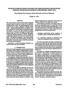
Figure 8: The state transition diagram on the right (a) depicts a stochastic automaton with two distinct sub automata. The automaton spends most of its time cycling between states 1 and 2, or cycling between states 3 and 4. The goal of slow feature analysis — as depicted in (b) — is to identify these sub automata and cluster the states accordingly. two states before entering an end state, it will require a DBN representing a K-level HHMM with O(2K ) slices to simulate one state transition in the top level. Fortunately, we can approximate such a HHMM with only O(K) space as illustrated in Figure 7.

5

Learning Invariant Features Using Inertial Priors

Before continuing with our discussion of embedded Markov models, we consider what it means to learn invariant features. Imagine a sequence of observations — quite likely noisy — and suppose the observations are of different shapes undergoing various transformations — quite likely nonlinear. Assume that consecutive observations in the sequence tend to come from observing the same shape undergoing the same transformation, but that periodically the shape or the transformation changes. Figure 8.a shows the state-transition diagram for a stochastic finite-state automaton characterizing this situation. The automaton has four states labeled 1 through 4 and three outputs labeled a, b and c. The edges in the diagram are labeled with transition probabilities, and following each transition the automaton emits the 9

Figure 9: This graphic illustrates the key components involved in learning a variable-order hidden Markov model embedded in a subnet. An observation model (a) maps input yit onto a set of atomic single-observation states σ ∈ Σ. A bounded-order hidden Markov process (b) is used to account for the evolution of the atomic single-observation states thereby modeling the transformations governing the input. The bounded-order Markov model over σ ∈ Σ is then mapped to a first-order Markov model (c) over a set of composite states ω ∈ Ω. The composite states are clustered (d) to form a set of output classes — the values of xti — so that composite states that tend to follow one another in time are in the same class. output associated with its current state. If we were to run this automaton, we would expect it to alternate between states 1 and 2 for a while, eventually transition to 4, alternate between 3 and 4 for a while, transition to 1, and so on. The two sets of states that are circled in Figure 8.b correspond to the sub automata on a given level in a hierarchical hidden Markov model. Learning the invariant feature of a subnet is tantamount to learning the sub automata governing the input to that subnet. To illustrate the process of learning invariant features, we examine a sequence of graphical models beginning with Figure 5, extending through four intermediate stages in Figure 9, and culminating in the final form shown in Figure 10. The first stage involves learning an observation model and is depicted in Figure 9.a. In order to enable learning invariants, we complicate the picture of the embedded Markov model in Figure 5 by introducing a new latent variable that mediates between the subnet hidden variable (xt1 ) and its set of observed variables (yit ). In describing the state space for this new latent variable, we find it useful to distinguish between the set of composite variable-duration states, denoted ω ∈ Ω, and the set of atomic single-observation states, 10

denoted σ ∈ Σ. Atomic states comprise our vocabulary for describing spatiotemporal patterns; think of the atomic states as the primitive symbols emitted by the sub automata in the hierarchical hidden Markov model. Composite states represent the variable-duration distinctive features of the temporal model; think of the composite states as the signature bigrams, trigrams and, more generally, n-grams that constitute our language for describing complex spatiotemporal patterns. t i signify the multivariate observation at time t. If the y are continuous, we might Let y t = hy11 , ..., yM i use a mixture of Gaussians to model the observations. The density relating observations to atomic states in this case is: H X p(yy |σ) = p(z = h|σ)p(yy |z = h) k=1

where p(yy |z = h) = N (yy |µh , Σh ) is a multivariate Gaussian and H is the number of mixture components. Unfortunately, only the level-one variables are continuous in our model. For all of the other levels in the hierarchy, the receptive-fieldQvariables in subnets are nominal valued, suggesting that we might be able to use naive Bayes, P (yy |σ) = M i=1 P (yi |σ), to model observations. It is important, however, that we be able to model the dependencies involving the variables in receptive fields. Instead of the traditional naive Bayes model, we use a variant of the tree-augmented naive Bayes networks of Friedman et al [21] to model observations: M Y P (yy |σ) = P (yi |Parents(yi ), σ) i=1

where Parents(yi ) denotes the set of parent nodes of yi in the graphical model determined by the Friedman et al algorithm. The Friedman et al algorithm serves to determine the set of intra-level edges that were left unspecified in the initial description of the underlying Bayesian network.3 Each level in the hierarchy tends to compress both space and time, inducing additional dependencies among the variables in the higher levels and rendering first-order models inappropriate. To account for these dependencies, we model the dynamics directly in terms of the atomic single-observation states using a bounded-memory Markov process with transition probabilities defined by P (σt |σt−1 , ..., σ0 ) = P (σt |σt−1 , ..., σt−L ) where L is the bound on the order of the Markov process. The resulting model is shown in Figure 9.b. with L = 3. To avoid the combinatorics involved in the use of higher-order models, we employ variable-order Markov models [57] to represent these long-range temporal dependencies. Variable-order Markov models have the advantage that they tend to require fewer parameters, and so provide some control over sample complexity.4 We use a continuous-input variant of the probabilistic suffix tree algorithm [57] following the work of Sage and Buxton [59] to learn a variable-order stochastic automaton modeling the underlying dynamics. The states of this automaton correspond to the leaves of the suffix tree and thus the composite variable-duration hidden states of our embedded Markov model.5 Each composite variable-duration state maps to a sequence of atomic single-observation states, ω ∈ Ω 7→ Σk for some k, and the transition probabilities are modeled as the first-order Markov process P (ωt |ωt−1 , ..., ω0 ) = P (ωt |ωt−1 ) shown in Figure 9.c. 3

We are also experimenting with a variant of the structural expectation maximization (SEM) algorithm [20] as a means of realizing a small subset of a much larger set of potential inter-level connections and implementing a version of Hebbian learning to establish inter-level edges. 4 Variable-duration hidden Markov models as described by Rabiner in [54] offer a representationally equivalent alternative, but tend to require more parameters. 5 Actually, the suffix tree has to be expanded to define a transition function on all pairs of states and symbols. Appendix B of [57] describes how to construct a probabilistic suffix automaton from the probabilistic suffix tree.

11

Figure 10: The four stages illustrated in Figure 9 can be combined a single graphical model whose parameters are learned by expectation maximization. The assignment of the conditional probability distribution for the variable xt1 , P (xt1 |xt−1 1 ), is governed in part by an inertial prior that biases parameter estimation in favor of models in which (the value of) xt1 tends to persist. The final form of the embedded hidden Markov model shown in Figure 9.d is determined by soft clustering the composite states to obtain the conditional probability P (ω1t |xt1 ). We apply a form of spectral analysis to the composite state transition matrix [50] and then apply soft K-means to the resulting vectors using greedy expectation maximization [63]. This final embedded model is related to the input/output hidden Markov model of Bengio and Frasconi [4] and the sparse Markov transducer of Eskin et al [15]. For purposes of exposition, we presented the embedded hidden Markov model in stages to illustrate the main components of the model. Indeed, learning embedded models in stages has certain advantages in terms of online and distributed implementations. However, it is possible and instructive to provide a graphical model that precisely specifies the topology of the network, as well as any assumptions in the form of prior knowledge required for inference. The key assumption in our model is that the features we are interested in learning change slowly even though the input is changing rapidly as a result of naturally occurring transformations. This is the assumption implicit in our use of spectral clustering to define P (ω1t |xt1 ). To make this assumption explicit in our model we first need to represent that the output at time t depends on the output at t − ∆. We do this by adding an arc from xt−∆ to xt in Figure 9.d to obtain the graphical model shown in Figure 10. To represent the bias that the output changes slowly, we introduce the notion of an inertial prior on the parameters of the (output) state transition matrix. Heckerman [26] introduced the likelihood equivalent uniform Bayesian Dirichlet (BDEU) metric as a means of scoring structures in learning Bayesian networks. To implement a prior using the BDEU metric, we first have to choose an equivalent sample size, which specifies the degree to which we expect the model parameters to change as we account for new evidence during parameter estimation. The equivalent sample size is converted into a matrix of pseudo counts weighted to account for the size of the conditional probability tables we are trying to learn. The pseudo counts are used during expectation maximization to adjust the expected sufficient statistics in updating the model parameters. Dirichlet priors serve as a regularizer and help to prevent over-fitting. To implement an inertial prior for the model in Figure 10, we simply re-weight the pseudo counts within the state-transition table representing P (xt |xt−∆ ) by fattening up the entries along the diagonal that govern self-transitions. With this additional bias, we can learn models that reliably identify and track the states of sub automata comprising the dynamics of subnet input. The method works across a range of processes and 12

Figure 11: An illustration of how temporal resolution is determined within a hierarchy of spatiotemporal features. Each of the four red boxes represents a sequence of output distributions of the binary hidden variable for some subnet. The shaded green bars provide an indication of the sampling rate for the subnets immediately upstream of the specified variables. is not sensitive to the parameter governing the re-weighting of diagonal entries.

5.1

Variable-duration Hierarchical Hidden Markov Models

Hierarchical hidden Markov models [18] allow us to model processes at different temporal resolutions. We could force each subnet to span a greater temporal extent than its children by having it sample the output of its children at intervals, rather than aligning the slices of its embedded hidden Markov model one-to-one with those of its children. In this section, we briefly explore another alternative that we are considering for the distributed implementation of our model. There is no need to specify distinct learning and inference phases in our model, but it is simpler to explain what is being learned if we make such a distinction. Assume for the sake of discussion, that learning proceeds one level of subnets at a time starting from bottom of the hierarchy. Each individual subnet receives a sequence of outputs (as described in Section 3) from each of the features associated with the nodes in its receptive field. During each primitive compute cycle, each subnet collects potentials from each of its neighbors in the subnet graph, updates its belief function, and produces an output. Each subnet also buffers some fixed number of outputs from the subnets in its receptive field. It is important to note, however, that while a subnet may produce an output at time t, that output need not be directly used in updating the subnets receiving that output — at least not in the sense that every output corresponds to a slice in some embedded hidden Markov model. If we assume that the period of the primitive compute cycle is short enough that we can recover the full Fourier spectrum of the signal underlying the sequence of outputs produced by any collection of subnets, then we use the Nyquist rate (twice the period of the highest frequency component in the Fourier spectrum) to determine the delay between atomic single-observation states.6 Figure 11 attempts to render this sampling process graphically. Each of the four red boxes in the figure depicts a sequence of output distributions of the hidden variable (binary in this example) for some subnet. The shaded green bars provide an indication of the sampling rate for the subnets immediately upstream of the specified variables. These samples correspond to the multivariate observations y t introduced earlier and serve to instantiate the slices in the embedded hidden Markov models. Given that the processes defined on Ω are first-order Markov (in contrast with the processes defined on Σ), we don’t actually have to keep around more than two slices since the past output history can now be summarized in a single slice. 6

There is evidence to suggest that cortex is capable of performing a similar sort of Fourier analysis as part of constructing spatial representations [39].

13

5.2

Balancing Selectivity and Invariance

Each subnet can now be viewed as identifying the sub automata responsible for its observed input. Suppose the atomic states Σ are associated with patterns of light and dark corresponding to simple shape fragments such as the following: . Consider the case of two subnets with adjacent receptive fields (1) (2) presented with the following sequences of inputs and producing x1 and x1 , respectively, as output:

(1)

(1)

(1)

(1)

(1)

(2)

The top subnet produces x1 for the sequence σ1 , σ2 , σ3 , σ4 and the bottom subnet produces x1 for (2) (2) (2) (2) the sequence σ1 , σ2 , σ3 , σ4 , since they have been trained on moving images and produce output that is invariant to translation. Suppose that a third subnet resides in the level above and takes as input the output of subnets one and (1) (2) two. Subnet three would see x1 and x1 and might classify this pattern as a somewhat longer bar tilted at approximately 5◦ off vertical and moving right (or up, e.g., see Figure 12), but what happens in the following:

(1)

(2)

In this case, subnets one and two might again output x1 and x1 , since they are trained to respond invariant with respect to translation. But then subnet three will respond exactly as before even though the input is not a continuous bar. Ullman and Soloviev resolve this dilemma by employing overlapping receptive fields. In their approach, subnet three would report a continuous canted bar only if this interpretation is consistent with all of the subnets spanning the relevant image region:

The output transition model P (xt |xt−1 ) responds invariant with respect to common transformations in the input allowing the model to generalize to novel stimuli. At the same time, the observation model P (yy |σ) selectively combines the output from several invariant features whose receptive fields overlap thereby preventing the model from over generalizing. The observation model also plays a key role in providing top-down priors by representing the dependencies among the receptive-field variables. We end this section with a brief discussion of some limitations and extensions of the approach described thus far. The first limitation concerns our ability to unambiguously capture the dynamics inherent in the input to a given subnet. Adelson and Movshon [1] discuss the aperture and temporal-aliasing problems which address the impossibility of simultaneously determining direction and velocity when viewing a moving object through a small-aperture window. Figure 12 illustrates the problem by showing a sequence of images 14

Figure 12: The problem of simultaneously determining the direction and velocity of an object when viewed through a small aperture is referred to as the aperture or temporal aliasing problem [1].

Figure 13: This graphic represents the atomic single-observation states corresponding to the bottom left-hand corner of an axis-aligned rectangle which is allowed to move left, right, up, down, and in either direction along any diagonal. The letters A–Q correspond to the atomic single-observation states in Σ. consistent with several different direction-velocity pairs. We simply accept this ambiguity on a given level, assuming that in most cases it will get resolved in subsequent levels of the hierarchy which enjoy a greater temporal and spatial extent. The second limitation concerns our ability to exploit the assumed temporal homogeneity of input sequences. Consider the depiction of Σ shown in Figure 13 and assume that the input sequence consists of sequences showing just the bottom right hand corner of an axis-aligned rectangle starting from an arbitrary point in the receptive field and moving left, right, up, down or back and forth along any diagonal. This is the sort of input and transformations that we are likely to see in the experiments described in Section 6. Note that the processes governing the transformations illustrated in Figure 13 are not first order. If a sequence of inputs starts in, say, J, the next inputs might be E, F , G, I, K, M , N , O or even J if the rectangle is not moving at all relative to the viewer’s frame of reference. However, if the viewer has seen the input M followed by J, then the next input is likely to be G. If a sequence begins in C, then D and a succession of Qs may follow. If it begins in B and the object is moving in the same direction, we’ll see C followed by D and then a succession of Qs. Ideally, we’d like to group B, C, D, Q∗ together with C, D, Q∗ since they are both generated by the same process. If the method of using variable-order Markov models performs as we expect it to, the subsequences B, C, D, Q and C, D, Q will be represented as separate composite variable-duration states. Moreover, if the inertial priors impose their bias as we have witnessed in other experiments, these two composite steps will be grouped by

15

the output variables of subnets. We have not as yet amassed enough experimental evidence to determine if this desired behavior can be achieved robustly. The next section provides a snapshot of where we are in terms of developing prototypes and running experiments.

6

Implementation

There is a great deal that we don’t know about the primate cortex. Indeed, it can be argued persuasively that we have a firm handle on as little as 10% of V1, which is arguably the most extensively studied area of the visual cortex [52]. Even so there is merit in developing large-scale simulations to test theories and explore practical applications. For the last year and a half, we have been working toward just such a goal. The models and algorithms described in the previous sections were designed for implementation on a computing cluster of the sort now relatively common in research labs: hundred-plus processors running at better than 2GHz, each having 2GB or more of memory and communicating though a fast interconnect, e.g., 10-Gigabit Ethernet. A single subnet with a 3 × 3 receptive field consisting of variables that can take on ten possible values can easily have conditional probability tables of size 105 , and exact inference using the junction-tree algorithm [10, 30] can involve cliques of size 107 or more depending on the arrangement of intra-level edges. If each subnet has a dedicated processor, a hierarchical model consisting of, say, four levels can process one input in less than 100 milliseconds assuming the sort of hardware outlined above. Since describing the basic approach in 2005 [11], we have built and experimented with several implementations. The first implementation was described in [12]; it uses a different topology for subnets and does not deal with time. This early prototype was written in Matlab and tested on the NIST hand-written digit database. The prototype managed a little better than 90% classification on the training data and better than 80% on the test data having seen only 1/3 of the available training data. This level of performance falls well short of the best algorithms but was not surprising given that our algorithm learned the parameters for all but the top-level subnet in an unsupervised manner. We also ran a set of experiments exploring the limitations of several layer-by-layer learning techniques and concluded that, without some form of supervision for the lower levels, significantly better performance is not possible. The results for these experiments as well as those for the digit recognition experiments are available on a web site created as a companion to this paper site http://www.cs.brown.edu/∼tld/projects/cortex/. Next we developed a prototype MPI-based7 version of the atemporal implementation as a proof of concept. The MPI version relied on running each subnet in a separate Matlab process and was useful primarily for debugging the message-passing algorithms in a distributed, asynchronous setting. We also implemented an initial temporal version using subnets with embedded hidden Markov models, but this version turned out to be impractical due in part to the size of the subnets employing the topology used in the early prototypes. The latest Matlab implementation includes all of the features described in this paper (including the new subnet topology) except the technique for automatically determining subnet sampling rates described in Section 5.1. The code for this implementation along with a study of models for learning invariants is available on the companion web site. In addition to experiments on the NIST digit database and various synthetic datasets, the on-line materials include a set of models and experimental results based on the pictionary dataset that was developed by Dileep George to test an implementation (see [23]) of hierarchical temporal memory [24, 25]. In the networks used in experiments with the pictionary dataset, the lowest level is 27 × 27, each subnet has a 3 × 3 receptive field, and there are no overlaps among the receptive fields. The nodes in each level are arranged in a square grid as shown in Figure 14.a, and subscribe to the fixed pattern of intra-level edges shown in Figure 14.b. 7

MPI (for “message-passing interface”) is a specification for parallel programming on a variety of hardware using a messagepassing protocol for interprocess communication.

16

    

n+1 ··· n + m + 1 ··· .. .. . . n + m2 − m · · · ··· n n+m .. .

n+m−1 n + 2m − 1 .. . n+

m2

    

−1

(a)

·→·→ ↓&↓& ·→·→ ↓&↓&

...

↓&↓& ·→·→

··· ··· ··· ···

→· &↓ →· &↓

...

&↓ →·

(b) Figure 14: One level in the Bayesian network used for the pictionary dataset illustrating (a) the nodenumbering scheme and (b) the pattern of intra-level connections showing how this pattern together with the node-numbering scheme ensure that the graph is acyclic and the natural ordering on the integers constitutes a topological sort of the nodes in the network. The width of a level is m = w + (p − 1)(w − o) where w is the width of the receptive fields, p is the width of the parent level and o is the overlap between adjacent receptive fields.

Figure 15: The forty-eight patterns comprising the pictionary dataset. These prototypes are used to generate sequences of images for evaluating invariant features.

17

Figure 16: A cross-sectional view of the hierarchical Bayesian network used for experiments involving the pictionary dataset showing a small portion of the 820 nodes that comprise this network. The resulting subnet graph consists of 91 subnets arranged in three levels, with a single subnet in level three, nine in level two, and 81 subnets in level one (see Figure 16). The binary images in the pictionary dataset are constructed from a set of forty-eight line drawings each representing a simple schematic shape, such as a bed, a cat, or the letter H, called a prototype (see Figure 15). To construct an image sequence, select a prototype shape, create the first frame in the sequence by positioning the prototype shape at a randomly chosen position in a 27 × 27 image field, select a transformation, and then obtain a sequence of frames by applying the selected transformation to frame i to obtain frame i + 1. The bottom two levels are trained in an unsupervised manner, and then the top level is trained in a supervised manner using the labels for the prototypes. In a typical experiment, we present the system with a thousand or so randomly generated sequences to train the bottom levels. Then we present an additional hundred or so sequences while assigning labels to the topmost node in the network which corresponds to the hidden node in the top subnet. We test the system by presenting an additional set of sequences and comparing the maximum a priori (MAP) value of the hidden node in the top-level subnet with the label of the last frame in the sequence. Performance is measured as the number of times the MAP estimate agrees with the label. If we consider eight possible transformations, say, translations up, down, left, right and along the diagonals, eight possible prototypes of size no more than 8 × 8, require that the first frame of any sequence completely contain the prototype, and constrain the length of the sequences to exactly five frames, then we have more than 20,000 training and testing examples to choose from. Randomly choosing from among the eight labels yields an expected performance of 12.5%. If we present 100 sequences of length five for a total of 500 frames we may not even see every prototype under all transformations. The Matlab implementation simulates a distributed system within a single Matlab process and can take a long time to train and test. To expedite the training and testing, we take several shortcuts: On level one, we tie the parameters across all of the 81 subnets and train just one subnet with 10,000 short sequences comprising approximately 25,000 individual frames. On level two, we partition the subnets into five groups covering separate regions of the visual field, tie the parameters of all the subnets within each group, and then train one subnet in each group selected so that it is centrally located within its region of the visual field. The single subnet in level three is trained in a supervised manner as described above. In the experiments described here, training proceeds level by level though this is not strictly necessary. Once a subnet is trained, it begins to receive messages containing potentials from its parents and children in the subnet graph. Trained subnets incorporate these potentials into their local belief function and propagate new potentials to their parents and children. When all of the subnets except those in the top level are trained, the top-level subnets (there is only one in the pictionary models) begin receiving potentials from their children and labels in the form of degenerate potentials (a vector with 0 in each position except the position corresponding the label index which is assigned 1) from the supervisory program in charge of supplying input to the bottom level and labels to the top level. Once the top-level subnets have accumulated enough training data, they begin to send potentials back to the supervisory program just as if it was their parent. These potentials are used to evaluate the performance of the network as a whole. Once all of the subnets have been trained, evaluation takes three cycles of inference per sequence frame, 18

# TESTING 500 400 600 500 600 500 500 500 500

# TRAINING 500 750 1000 1250 1500 1750 2000 2500 2750

% CORRECT 35.56% (64/180) 38.36% (56/146) 45.21% (99/219) 40.56% (73/180) 47.20% (101/214) 51.40% (92/179) 46.99% (86/183) 53.55% (98/183) 55.49% (101/182)

ELAPSED TIME 32614 seconds (approximately 9 hours) 47319 seconds (approximately 13 hours) 62279 seconds (approximately 17 hours) 83434 seconds (approximately 23 hours) 89734 seconds (approximately 25 hours) 105910 seconds (approximately 29 hours) 163943 seconds† (approximately 46 hours) 199477 seconds† (approximately 55 hours) 189110 seconds† (approximately 53 hours)

Table 1: Shown are the results from nine experiments using the pictionary dataset. Each experiment uses eight of the forty-eight prototypes in the dataset, and so random guessing yields 12.5% in expectation. The columns in the table correspond to the number of frames used for training, the number frames used for testing, the percentage of sequences in which the MAP assignment for the last frame in a sequence matches the label of the prototype being transformed in the sequence, and, finally, the elapsed time required to run the experiment (all jobs except those marked with † were run on a dedicated processor). one cycle for each level as messages are passed up the hierarchy. For pictionary evaluation, we don’t bother with passing messages back down the hierarchy as we are only concerned with the belief function computed by the top-level subnets. This implies that processing each frame requires 91 subnets to update their belief functions and pass messages. Performing these 91 updates serially can take considerable time. On a dedicated 2GHz processor with 2GB of memory, training and testing, including both learning and inference for all but the first level (which is trained separately so that its parameters can be reused in several experiments), takes about one minute per frame. For example, an experiment involving 1500 frames takes a little over 24 hours. This has limited the size and type of experiments we have been able to run and has motivated our work on implementations that can take advantage of distributed computing — more about which subsequently. Nevertheless we have performed many smaller experiments and we have made our Matlab implementation available on the companion web site for others to replicate our experiments and conduct their own. Table 1 shows the results of nine representative experiments; more results are available on the companion web site along with the code used to produce them. The level of performance is respectable given the small amount of training data used and the fact that these results required no tuning of parameters, unless one counts the rather Draconian step of tying the parameters in levels one and two to achieve reasonable running time (which is more likely to impact adversely performance). These results rely exclusively on first-order and zero-order models even though, as pointed out in Section 5.2, the transformations in our experiments are likely best modeled as second-order processes. The first implementation (in Matlab) for learning variableorder Markov processes using inertial priors and the DBN shown in Figure 10 required approximately 20 minutes to train on 10,000 sequences of average length 5 and an alphabet of 25. Doubling the alphabet size increases the time fivefold, while time scales linearly with the number of sequences. The latest version which decomposes training into three stages depicted in Figure 4.b and the models shown in Figure 9 is written largely in C and takes less than a minute to train on 10,000 sequences of average length 5 and an alphabet of 25. More important than our not using variable-order models is the fact that we use first-order models only on level one; the models in subnets on levels two and three are zero-order.8 The first-order subnets on level 8

This choice of models was forced on us by memory limitations and our single-minded pursuit of a parallel implementation.

19

one can take advantage of their inertial priors to support the sort of semi-supervised learning described in Section 5. Learning in the zero-order subnets on level three is facilitated through the use of labels. The zero-order subnets on level two, however, have neither labels nor informative priors to guide learning. We are confident that we can significantly improve upon the results shown in Table 1 by using first-order models in the subnets on level two. At this point, we are concentrating on a C++ implementation that will free us from our dependence on Matlab and, in particular, on having to manage all of the subnets within a single process running on a single machine. The current Matlab implementation owes much to Kevin Murphy’s Bayes Net Toolbox (BNT) [46]. Happily, we were able get a good deal of the functionality of BNT by using Intel’s open-source Probabilistic Networks Library (PNL) http://www.intel.com/technology/computing/pnl/index.htm which drew upon BNT for inspiration and technical detail. It is hard to beat Matlab in performing basic vector and matrix operations, but we achieve close to the same level of performance on these operations using a C++ interface to the BLAS and LAPACK Fortran libraries which Matlab also leverages for this purpose. The initial attempts to parallelize our code using MPI/LAM [9] were frustrated by the low-level nature of MPI and the overhead involved in porting to various clusters. We are now collaborating with three engineers at Google to take advantage of Google’s considerable computational resources and the layer of software that shelters Google application programmers from the annoying details of processor allocation and inter-processor communication. As results become available, they will be reported on the companion web site.

7

Discussion and Related Work

The main contribution of this paper is a class of probabilistic models and an associated bias for learning invariant features. Instances of this class can be embedded as components within a more comprehensive hierarchical model patterned after the visual cortex and approximating a hierarchical hidden Markov model. We have mentioned much of the directly related work in the context of the preceding discussion. Here we review additional relevant work and then conclude with a discussion of what we believe to be some of the most important remaining technical challenges. Wiskott and Sejnowski [65] present a neurally-inspired approach to learning invariant or slowly-varying features from time-series data. It was their intuition which first led us to pursue the line of research explored in this paper: “The assumption is that primary sensory signals, which in general code for local properties, vary quickly while the perceived environment changes slowly. If one succeeds in extracting slow features from the quickly varying sensory signal, one is likely to obtain an invariant representation of the environment.” Later we encountered the earlier work of F¨oldi´ak providing an account [19] of Hebbian learning in complex cells in which the output of a cell is adjusted in accord with its output at the previous time step: “This temporal low-pass filtering of the activity embodies the assumption that the desired features are stable in the environment.” Hawkins and George [25] stress the importance of “spatial and temporal pooling” in training their hierarchical temporal models. Hawkins [24] presents a general cortical model that incorporates variants of many of the basic ideas presented above, and George and Hawkins [23] describe a preliminary implementation of the Hawkins’ model. Their implementation does not employ a temporal model per se despite their stated emphasis on identifying frequently occurring sequences generated by a common cause. By using a When run in a single Matlab process, the simulated distributed model with first-order subnets on both level one and level two requires seven gigabytes just to store the model parameters. Our mindset all along has been that we must implement our model to run on parallel hardware if we are to demonstrate its merits convincingly on interesting problems, and, clearly, pictionary is a toy problem meant to emphasize the task of learning invariants. This mindset has allowed us to focus on developing parallel codes, but it has also deflected us from developing efficient serial codes.

20

more expressive temporal model, we are able to represent a richer set of causes and thus potentially improve generalization. They also rely on tree-structured Bayesian networks with their obvious computational advantages and representational shortcomings (they do not allow overlapping receptive fields or intra-level edges). Wiskott and Sejnowski impose what we have referred to as inertial priors to bias learning to find invariant features. Inertial priors together with the assumption of local homogeneity enable a form of semi-supervised learning. Inputs corresponding to instantiations of receptive-field variables are obviously not labeled. However, we assume that inputs in close temporal proximity will tend to be associated with the same cause, as Hawkins might characterize it, and, hence, they have the same label. Bray and Martinez [8] implement a form of inertial bias by maximizing output variance over the long term while minimizing output variance over the short term. Kab´an and Girolami [36] provide an alternative approach based on generalized topographic maps [6] for exploiting locally homogeneous regions of text in documents. Our approach to modeling time using variable-duration Markov models allows us to implement inertial priors directly within the underlying Bayesian graphical model. Psychologists have long been interested in how subjects group objects in space and time. Kubovy and Gepshtein [38] review the psychophysical evidence for current theories about how we group objects according to their spatial and temporal proximity. Their discussion of Shimon Ullman’s early work was particularly helpful in thinking about learning spatiotemporal features. Our inspiration for modeling the visual cortex as a hierarchical Bayesian network came from [42]. In the simplest instantiation of the Lee and Mumford model within our framework, each subnet is of the form P (xi |xi+1 ) and (exact) inference can be accomplished using Pearl’s belief propagation algorithm [53] by passing λ messages P (ξ − |xi ) to subnets upstream in the visual pathway, and π messages P (xi+1 |ξ + ) downstream, where ξ + and ξ − represent the evidence originating, respectively, above and below in the hierarchy. Overlapping receptive fields and intra-level edges necessarily complicate this simple picture. In particular, separate subnets may not assign the same potentials to nodes in the intersection of their respective receptive fields. Different subnets may even impose different local topologies over the same variables since connectivity among receptive field variables is learned independently. While we originally viewed the ability of subnets to impose different local topologies on their shared variables as a liability, we now view it as a feature of our model that contributes to its robustness. However, we do take steps to ensure that subnets agree, at least approximately, on the potentials they assign to shared variables. Partial agreement is accomplished by having subnets with overlapping receptive fields exchange potentials. This exchange occurs prior to each update of the local belief function which occurs twice per input, once on passing potentials up the hierarchy starting from the input level and once on passing potentials back down the hierarchy. Since the receptive fields of subnets in the higher levels span large portions of their respective levels, this means that information tends to spread more quickly among the nodes at the highest levels. A subnet with hidden variable x receives potentials corresponding to priors of the form P (x|ξ) from all of the subnets whose receptive fields contain x; to resolve any remaining differences, these potentials are combined into a single potential as a weighted average. There is no shortage of proposals suggesting variants of the sort of level-by-level learning that we have used in our algorithms. In particular, Hinton turned to hierarchical learning in restricted Boltzmann machines as a means of tractable inference. Restricted Boltzmann machines are a special case of the product of experts (PoE) model [27]. In PoEs, the hidden states are conditionally independent given the visible states just as they are in our networks. Mayraz and Hinton [43] suggest the use of the following strategy for learning these multi-layer models: “Having trained a one-hidden-layer PoE on a set of images, it is easy to compute the expected activities of the hidden units on each image in the training set. These hidden activity vectors will themselves have interesting statistical structure because a PoE is not attempting to find 21

independent causes and has no implicit penalty for using hidden units that are marginally highly correlated. So we can learn a completely separate PoE model in which the activity vectors of the hidden units are treated as the observed data and a new layer of hidden units learns to model the structure of this ‘data’.” A number of researchers have made similar observations and put forward proposals for performing inference that exploit the same underlying intuitions. We were originally attracted to the idea of level-by-level parameter estimation in reading [23] although the basic idea is highly reminiscent of the interactive activation model described in [44]. In the George and Hawkins algorithm, each node in a Bayesian network collects instantiations of its children that it uses to derive the state space for its associated random variable, and estimate the parameters for the conditional probability distributions of its children. The states that comprise the state space for a given node correspond to perturbed versions of the most frequently appearing vectors of instantiations of its children. Their network is singly connected and, for this class of graphs, Pearl’s belief-propagation algorithm is both exact and efficient. Hinton, Osindero and Teh [29] present a hybrid model combining Boltzmann machines and directed acyclic Bayesian networks. They also employ level-by-level parameter estimation in an approach similar to the algorithm for learning restricted Boltzmann machines mentioned earlier. They apply Hinton’s method of contrastive divergence in an attempt to ensure that units within a layer are diverse in terms of the features they model and various methods of isolating and tying parameters to control convergence. We expect that for many perceptual learning problems the particular way in which we decompose the parameter-estimation problem (which is related to Hinton’s weight-sharing and parameter-tying techniques) will avoid potential problems due to early (and permanently) assigning parameters to the lower layers. Yann LeCun and his colleagues [41] have developed a class of models called Multi-Layer Convolutional Neural Networks that are trained using a version of the back-propagation algorithm [58] and have been shown to be effective in object recognition [40]. Fei-Fei and Perona [17] have a Bayesian approach to learning hierarchical models for recognizing natural scene categories [16]. In an important sense, the main technique presented in this paper is a one-trick pony. Our basic premise is that inertial priors can turn an unsupervised learning problem into a semi-supervised problem, assuming that the basic underlying assumptions apply. All of the other pieces depend on this one, rather simple idea. We believe that the best way to amplify the value of inertial priors is to combine this bias with attentional mechanisms so that, in addition to exploiting the assumption that world changes slowly, we force the world, or rather our perception of the world, to change under our control, for example, by moving our eyes or our bodies. By making use of our ability to intervene in the world, we can very often resolve perceptual ambiguity. Indeed, in many cases, it is only by engaging the world that we can obtain the information needed to self-supervise our learning.

8

Acknowledgments

Thanks to David Mumford and Tai-Sing Lee for the paper that inspired this work and my interest in computational neuroscience. Students at Brown and Stanford, including Arjun Bansal, Chris Chin, Jonathan Laserman, Aurojit Panda, Ethan Schreiber and Theresa Vu, helped debug both the ideas and the various implementations. Dileep George and Bobby Jaros at Numenta provided feedback on early versions of the temporal model, and Jeff Hawkins provided insight on the neural and algorithmic basis for spatiotemporal pooling. At Google, Glenn Carroll, Jim Lloyd and Rich Washington always asked just the right questions to get me back on track when I was confused. Mark Boddy and Steve Harp at Adventium Labs provided insights into the application of cortical models to the game of Go. Finally, I am grateful to Johan de Kleer, Tom

22

Mitchell, Nils Nilsson, Peter Norvig and Shlomo Zilberstein for their early encouragement in my pursuing this research.

References [1] A DELSON , E., AND M OVSHON , J. Phenomenal coherence of moving visual patterns. Nature 300 (1982), 523–525. [2] BARTO , A. G., S UTTON , R. S., AND A NDERSON , C. W. Neuronlike adaptive elements that can solve difficult learning control problems. IEEE Transactions on Systems, Man, and Cybernetics 13, 5 (1983), 835–846. [3] BASYE , K., D EAN , T., K IRMAN , J., AND L EJTER , M. A decision-theoretic approach to planning, perception, and control. IEEE Expert 7, 4 (1992), 58–65. [4] B ENGIO , Y., AND F RASCONI , P. An input output HMM architecture. In Advances in Neural Information Processing 6, e. a. J. D. Cowan, Ed. Morgan Kaufmann, San Francisco, California, 1994. [5] B ERKES , P., AND W ISKOTT, L. Slow feature analysis yields a rich repertoire of complex cell properties. Journal of Vision 5, 6 (2005), 579–602. [6] B ISHOP, C. M., S VENS E´ N , M., AND W ILLIAMS , C. K. I. GTM: A principled alternative to the selforganizing map. In Advances in Neural Information Processing Systems, M. C. Mozer, M. I. Jordan, and T. Petsche, Eds., vol. 9. MIT Press, Cambridge, MA, 1997, pp. 354–360. [7] B RAITENBERG , V., AND S CHUZ , A. Cortex: Statistics and Geometry of Neuronal Connections. Springer-Verlag, Berlin, 1991. [8] B RAY, A., AND M ARTINEZ , D. Kernel-based extraction of slow features: Complex cells learn disparity and translation invariance from natural images. In Advances in Neural Information Processing Systems, vol. 14. MIT Press, Cambridge, MA, 2002. [9] B URNS , G., DAOUD , R., AND VAIGL , J. LAM: An open cluster environment for MPI. In Proceedings of Supercomputing Symposium (1994), pp. 379–386. [10] C OWELL , R. G., DAWID , A. P., L AURITZEN , S. L., AND S PIEGELHALTER , D. J. Probabilistic networks and expert systems. Springer-Verlag, New York, NY, 1999. [11] D EAN , T. A computational model of the cerebral cortex. In Proceedings of AAAI-05 (Cambridge, Massachusetts, 2005), MIT Press, pp. 938–943. [12] D EAN , T. Scalable inference in hierarchical generative models. In Proceedings of the Ninth International Symposium on Artificial Intelligence and Mathematics (2006). [13] D EAN , T., AND K ANAZAWA , K. A model for reasoning about persistence and causation. Computational Intelligence Journal 5, 3 (1989), 142–150. [14] E LIDAN , G., M C G RAW, I., AND KOLLER , D. Residual belief propagation: Informed scheduling for asynchronous message passing. In Proceedings of the Twenty-second Conference on Uncertainty in AI (UAI) (Boston, Massachussetts, July 2006).

23

[15] E SKIN , E., G RUNDY, W. N., AND S INGER , Y. Protein family classification using sparse markov transducers. In Proceedings of the Eighth International Conference on Intelligent Systems for Molecular Biology (2000), pp. 134–145. [16] F EI -F EI , L., F ERGUS , R., AND P ERONA , P. Learning generative visual models from few training examples: an incremental Bayesian approach tested on 101 object categories. In Proceedings of CVPR05 Workshop on Generative-Model Based Vision (2004). [17] F EI -F EI , L., AND P ERONA , P. A Bayesian hierarchical model for learning natural scene categories. In CVPR (2005). [18] F INE , S., S INGER , Y., AND T ISHBY, N. The hierarchical hidden Markov model: Analysis and applications. Machine Learning 32, 1 (1998), 41–62. ¨ ´ , P. Learning invariance from transformation sequences. Neural Computation 3 (1991), AK [19] F OLDI 194–200. [20] F RIEDMAN , N. The Bayesian structural EM algorithm. In Proceedings of the Conference on Uncertainty in Artificial Intelligence (1998), pp. 129–138. [21] F RIEDMAN , N., G EIGER , D., AND G OLDSZMIDT, M. Bayesian network classifiers. Machine Learning 29, 2-3 (1997), 131–163. [22] F UKUSHIMA , K. Neocognitron: A self organizing neural network model for a mechanism of pattern recognition unaffected by shift in position. Biological Cybernnetics 36, 4 (1980), 93–202. [23] G EORGE , D., AND H AWKINS , J. A hierarchical Bayesian model of invariant pattern recognition in the visual cortex. In Proceedings of the International Joint Conference on Neural Networks, vol. 3. IEEE, 2005, pp. 1812–1817. [24] H AWKINS , J., AND B LAKESLEE , S. On Intelligence. Henry Holt and Company, New York, 2004. [25] H AWKINS , J., AND G EORGE , D. Hierarchical temporal memory: Concepts, theory and terminology, 2006. [26] H ECKERMAN , D. A tutorial on learning Bayesian networks. Tech. Rep. MSR-95-06, Microsoft Research, 1995. [27] H INTON , G. Product of experts. In Proceedings of International Conference on Neural Networks (1999), vol. 1, pp. 1–6. [28] H INTON , G., AND S EJNOWSKI , T. Learning and relearning in Boltzmann machines. In Parallel Distributed Processing: Explorations in the Microstructure of Cognition, Volume I: Foundations. MIT Press, Cambridge, Massachusetts, 1986, pp. 282–317. [29] H INTON , G. E., O SINDERO , S., AND T EH , Y.-W. A fast learning algorithm for deep belief nets. Neural Computation (2006). [30] H UANG , C., AND DARWICHE , A. Inference in belief networks: A procedural guide. International Journal of Approximate Reasoning 15, 3 (1996), 225–263. [31] H UBEL , D. H. Eye, Brain and Vision (Scientific American Library, Number 22). W. H. Freeman and Company, 1995. 24

[32] H UBEL , D. H., AND W IESEL , T. N. Receptive fields, binocular interaction and functional architecture in the cat’s visual cortex. Journal of Physiology 160 (1962), 106–154. [33] JACKENDOFF , R. Foundations of Language: Brain, Meaning, Grammar, Evolution. Oxford University Press, Oxford, UK, 2002. [34] J ENSEN , F. Bayesian graphical models. John Wiley and Sons, New York, NY, 2000. [35] J ORDAN , M., Ed. Learning in Graphical Models. MIT Press, Cambridge, MA, 1998. ´ , A., AND G IROLAMI , M. A dynamic probabilistic model to visualise topic evolution in text [36] K AB AN streams. Journal of Intelligent Information Systems 18, 2-3 (2003), 107–125. [37] K EARNS , M., AND VALIANT, L. G. Cryptographic limitations on learning boolean functions and finite automata. In Proceedings of the Twenty First Annual ACM Symposium on Theoretical Computing (1989), pp. 433–444. [38] K UBOVY, M., AND G EPSHTEIN , S. Perceptual grouping in space and in space-time: An exercise in phenomenological psychophysics. In Perceptual Organization in Vision: Behavioral and Neural Perspectives, M. Behrmann, R. Kimchi, and C. R. Olson, Eds. Lawrence Erlbaum, Mahwah, NJ, 2003, pp. 45–85. [39] K ULIKOWSKI , J. J., AND B ISHOP, P. O. Fourier analysis and spatial representation in the visual cortex. Experientia 37 (1981), 160–163. [40] L E C UN , Y., H UANG , F.-J., AND B OTTOU , L. Learning methods for generic object recognition with invariance to pose and lighting. In Proceedings of IEEE Computer Vision and Pattern Recognition (2004), IEEE Press. [41] L E C UN , Y., M ATAN , O., B OSER , B., D ENKER , J. S., H ENDERSON , D., H OWARD , R. E., H UB BARD , W., JACKEL , L. D., AND BAIRD , H. S. Handwritten zip code recognition with multilayer networks. In Proceedings of the International Conference on Pattern Recognition (1990), IAPR, Ed., vol. II, IEEE Press, pp. 35–40. [42] L EE , T. S., AND M UMFORD , D. Hierarchical Bayesian inference in the visual cortex. Journal of the Optical Society of America 2, 7 (July 2003), 1434–1448. [43] M AYRAZ , G., AND H INTON , G. Recognizing handwritten digits using hierarchical products of experts. IEEE Transactions on Pattern Analysis and Machine Intelligence 24 (2002), 189–197. [44] M C C LELLAND , J., AND RUMELHART, D. An interactive activation model of context effects in letter perception: I. An account of basic findings. Psychological Review 88 (1981), 375–407. [45] M URPHY, G. L. The Big Book of Concepts. MIT Press, Cambridge, MA, 2002. [46] M URPHY, K. The Bayes Net Toolbox for Matlab. Computing Science and Statistics 33 (2001). [47] M URPHY, K., W EISS , Y., AND J ORDAN , M. Loopy-belief propagation for approximate inference: An empirical study. In Proceedings of the 16th Conference on Uncertainty in Artificial Intelligence (2000), Morgan Kaufmann, pp. 467–475. [48] M URPHY, K. P. Dynamic Bayesian Networks: Representation, Inference and Learning. PhD thesis, University of California, Berkeley, Computer Science Division, 2002. 25

[49] M URRAY, S. O., O LSHAUSEN , B. A., AND W OODS , D. L. Processing shape, motion and threedimensional shape-from-motion in the human cortex. Cerebral Cortex 13, 5 (2003), 508–516. [50] N G , A., J ORDAN , M., AND W EISS , Y. On spectral clustering: Analysis and an algorithm. In Advances in Neural Information Processing Systems (Cambridge, MA, 2002), vol. 14, MIT Press. [51] O LSHAUSEN , B. A., A NDERSON , A., AND VAN E SSEN , D. C. A neurobiological model of visual attention and pattern recognition based on dynamic routing of information. Journal of Neuroscience 13, 11 (1993), 4700–4719. [52] O LSHAUSEN , B. A., AND F IELD , D. J. How close are we to understanding V1? Neural Computation 17 (2005), 1665–1699. [53] P EARL , J. Probabilistic Reasoning in Intelligent Systems: Networks of Plausible Inference. Morgan Kaufmann, San Francisco, California, 1988. [54] R ABINER , L. R. A tutorial on hidden Markov models and selected applications in speech recognition. Proceedings of the IEEE 77, 2 (1989), 257–286. [55] R IESENHUBER , M., AND P OGGIO , T. Hierarchical models of object recognition in cortex. Nature Neuroscience 2, 11 (November 1999), 1019–1025. [56] R IVEST, R. L., AND S LOAN , R. A formal model of hierarchical concept learning. Information and Computation 114, 1 (1994), 88–114. [57] RON , D., S INGER , Y., AND T ISHBY, N. The power of amnesia: Learning probabilistic automata with variable memory length. Machine Learning 25, 2-3 (1996), 117–149. [58] RUMELHART, D. E., H INTON , G. E., AND W ILLIAMS , R. J. Learning internal representations by error propagation. In Parallel Distributed Processing: Explorations in the Microstructure of Cognition. Volume 1: Foundations, D. E. Rumelhart and J. L. McClelland, Eds. MIT Press, Cambridge, MA, 1986. [59] S AGE , K. H., AND B UXTON , H. Joint spatial and temporal structure learning for task based control. In International Conference on Pattern Recognition (ICPR) (2004), vol. 2, pp. 48–51. [60] U LLMAN , S. The Interpretation of Visual Motion. MIT Press, Cambridge, MA, USA, 1979. [61] U LLMAN , S., AND S OLOVIEV, S. Computation of pattern invariance in brain-like structures. Neural Networks 12 (1999), 1021–1036. [62] VALIANT, L. G. A theory of the learnable. Communications of the ACM 27 (1984), 1134–1142. ¨ , B. Efficient greedy learning of gaussian mixtures. Neural [63] V ERBEEK , J., V LASSIS , N., AND K R OSE Computation 15, 2 (2003), 469–485. [64] W ERTHEIMER , M. Untersuchungen zur lehre von der gestalt, II (Investigations of the principles of gestalt, II). Psychologische Forschung 4 (1923), 301–350. [65] W ISKOTT, L., AND S EJNOWSKI , T. Slow feature analysis: Unsupervised learning of invariances. Neural Computation 14, 4 (2002), 715–770. [66] Y EDIDIA , J. S., F REEMAN , W. T., AND W EISS , Y. Understanding belief propagation and its generalizations. In Exploring artificial intelligence in the new millennium, G. Lakemeyer and B. Nebel, Eds. Morgan Kaufmann Publishers Inc., San Francisco, 2003, pp. 239–269.

26