Learning By Investing Embodied Technology and Business Cycles Geng Li

∗

Federal Reserve Board May 2011

Abstract Major technological advances often require investment in new capital before they raise productivity. The extent to which productivity can be raised, however, is often unknown at the arrival of the new technology. This paper develops a dynamic model of optimal investment with technological advances of unknown magnitude and strong complementarity between new capital and new technology. In such a model the productivity frontier after a technological advance is learnt from sequentially assessing returns on new capital invested in the previous period. Motivated by the IT-related investment boom and bust, a closed-form sufficient condition for accelerating investment that induces a capital overhang is derived. Simulation results show that sufficiently large technological advances can induce long-lasting expansions and endogenous recessions in this model.

KEYWORDS: Embodied technology, Learning, Overinvestment, AK models JEL Classification: E22, E32

∗

Federal Reserve Board, Washington, DC 20551. Email [email protected]. This is a revised version of a chapter from my dissertation. I am deeply indebted to my dissertation committee members—Robert Barsky, Matthew Shapiro, Dmitriy Stolyarov and Tyler Shumway—for their guidance and encouragements. I also thank Susanto Basu, Karen Dynan, James Feigenbaum, Andra Ghent, Chris House, Miles Kimball, many of my colleagues at the Federal Reserve Board, the participants of seminars and conferences where the paper was presented at various stages, and in particular, Bob King, and an anonymous referee for helpful suggestions and comments. The views presented in the paper are those of the author and are not necessarily those of the Federal Reserve Board or its staff.

1

Introduction

Most technological advances require investment in new capital before the economy can enjoy a higher productivity. In the polar case, new technology and new capital can be complements in a Leontief way. In such a scenario output does not increase after a new technology arrives if no new capital is installed. Properties of such strong complementarity between new technology and new capital, which is often referred to as embodied technology, has been explored since at least Solow (1959). In this paper, we study a model that is different from canonical embodied technology models in three key aspects. First, standard embodied technology models assume that new technology only applies to the capital installed after the technological advance, leaving the productivity of older capital unchanged. In contrast, we assume that new technology raises the productivity of capital of all vintages once new capital is installed. Second, marginal product of capital does not change with the amount of new capital installed in standard models. We assume instead that, up to the frontier of the underlying technological advance, the more new capital has been installed, the more productivity gains are materialized. Finally, unlike standard models that assume the magnitude of the technological advance is known at its arrival, we assume that the magnitude is not known immediately at the arrival of the advance. The magnitude instead will be learned gradually through investing in new capital and assessing the induced increase of productivity. Specifically, in our model when a technological advance arrives, productivity, which applies to capital of all vintages, becomes an increasing function (the embodiment function) of the amount of new capital invested, up to a limit determined by the magnitude of the advance itself. Beyond this limit, investment in new capital no longer increases productivity. Investors only know the distribution from which the technology shock is drawn but do not observe its exact magnitude. Therefore, investment is made based on imperfect information about the size of the shock. Each period, investors find out whether they have invested enough in new capital to take the full advantage of the new technology by assessing the productivity gains induced by the investment made last period. If the potential of the new technology has not been reached, investors’ belief on the magnitude of the underlying advance will be updated and the investment in new capital will continue. In its spirit, the model is closely related to Zeira (1987), in which capital productivity declines to zero beyond an ex ante unknown upper bound of productive capital. We will discuss in more detail how our model is related to Zeira (1987) later in the paper. In addition, we show that, under certain assumptions of the embodiment function, the production function introduced here is equivalent to an AK model with an ex ante unknown boundary,

1

beyond which the production technology is concave, instead of linear, in capital. Our model of investment dynamics in the wake of major technological advances is, to a great extent, motivated by the accelerating investment in new capital and capital overhang during the IT boom and bust. Private investment rose substantially in terms of both levels and its share in GDP in the 1990s and such growth stopped abruptly in the year 2000. In the subsequent years, investment decreased sharply and the economy as a whole experienced a recession. Many business leaders and policymakers concluded that aggressive investment in IT and related industries during the boom largely resulted in a substantial overhang of capital.1 The model introduced in this paper can replicate qualitatively the key features of this episode of expansion and contraction. Heuristically, firms invest in new capital to take advantage of the IT revolution, without knowing the limit to which this new technology can increase productivity. The belief of this limit becomes increasingly optimistic over time as investors repeatedly realize that they have not invested enough to exhaust the potential of the new technology. Such belief revisions lead to increasingly aggressive investment and a capital overhang, followed by a recession. Formally, a closedform sufficient condition for accelerating investment is derived for our model. We show, for example, if the economy has CRRA preferences and the technology shock is believed to be drawn from a Cauchy distribution, our model implies accelerating investment. The way technological advances raise productivity and the information structure introduced in this model makes output react to technology shocks with greater inertia than in the equilibrium business cycle models that do not have these features. We show that in our model a single sufficiently large technological advance can induce a decade-long economic expansion that ends with overinvestment, exemplifying the model’s strong propagation mechanism. In our model, recessions arise endogenously, instead of being driven by negative shocks. To this extent, a favorable technology innovation already contains the seed of a future recession. Moreover, one implication of the model is that experiencing such recessions, though ex post costly, is ex ante optimal. It should be noted that the technology shocks feeded into the impulse-response analysis in our paper are somewhat different from those used in most business cycle studies (such as the Solow residual series). 1

For example, in July 2000, close to the peak of the boom, Microsoft President and CEO Steve Ballmer commented in a speech to the technology association of Georgia that, “A lot of people are overinvesting in dot-com start-ups ... There has been a hysteria. There is too much money chasing Internet ideas in the short run.”, Likewise, one year later, after the investment spending boom collapsed and the economy was in a recession, the then vice chairman of the Federal Reserve Board, Roger W. Ferguson, commented on July 18, 2001 in a speech to the Charlotte Economics Club that “ ... for a variety of reasons ... firms may be holding considerably more capital now than they would prefer . . . although it is difficult to determine how large the overhangs of capital might be at present, they seem likely to exert at least a modest amount of drag on the economy over the near term, even as growth picks up.”

2

Our model is most applicable in describing the investment dynamics with respect to the revolutionary technological advances that have profound and extensive impact on the economy, which are often referred to as the general purpose technology (GPT).2 Accordingly, our simulation analysis focus on the economy’s response during one episode of such a GPT advance. The paper will proceed as follows. Section 2 sets up the model of embodied technology and learning and introduces an embodiment function that exhibits certain useful properties. Section 3 presents the key properties of the model, including a sufficient condition for accelerating investment. For expositional purposes, we study the investment dynamics after a technological advance of both known and unknown magnitude. Section 4 discuss in great detail the model’s relationship to previous models of embodied technology (such as Solow 1959) and models of investment under uncertainty (such as Zeira 1987). Section 5 presents some numerical examples when the model is more realistically parameterized and shows that the model can replicate qualitatively the key observations from the IT boom and bust. Finally, Section 6 concludes and sets forth a research agenda.

2

A Model of Embodied Technology and Learning

2.1

Production Function and Information Structure

We begin with formalizing the key assumptions of our model introduced at the beginning of the paper regarding technology-capital complementarity and information structure. Assumption 1 Investment in new capital is required to take advantage of new technology. Productivity increases with the quantity of new capital invested up to a limit that is determined by the magnitude of the underlying technological advance. Assumption 2 As new capital is accumulated, productivity of both old and new capital increases. Assumption 3 Investors know only the distribution of technological advances, but do not know the magnitude of a realized advance at its arrival. Assumption 4 A firm can learn only through its own experiments and cannot learn from other firms. Now we show how each assumption is factored into the model: Assume that a technological advance arrives at t = 0, before which the production function of a representative firm is Y0 = A0 × K0α ,

(1)

2 Jovanovic and Rousseau (2005) provide a comprehensive treatment of the GPT history and its contributions to economic growth.

3

where Y0 is the output, and K0 is the pre-shock level of capital that is assumed to be at the steady state level with respect to the pre-shock level of technology, A0 . The post-shock level of technology is denoted by A and A > A0 . After the technological advance arrives, the production function becomes et × K α Yt = A t

∀

t>0,

(2)

et = min [A, Ψ (Knew, t , Kold, t )] is the effective productivity in period t. It is equal to the minwhere A imum between A, the underlying post-shock frontier of technology, and Ψ (Knew, t , Kold, t ), a function capturing how much of the new technology has been embodied into new capital invested. Consistent with Assumption 1, the embodiment function Ψ should satisfy Ψ(0, Kold ) = A0 , and

∂Ψ ≥ 0, ∂Knew

(3)

so that without any investment in new capital productivity does not rise, and that productivity increases with the amount of new capital invested up to a limit. It is clear that relative to the old capital that existed before the arrival of new technology, new capital bears an additional role—embodying new technology. Therefore, the marginal product of new capital always (at least weakly) exceeds that of old capital. Assuming there is no depreciation, all post-shock investment will be made in new capital. The amount of old capital will therefore be a constant equal to K0 . Thus, the embodiment function can be presented as Ψ(Kt , K0 ), where total capital stock, Kt = Knew,t + Kold,t , evolves as Kt = K0 + Knew, t = K0 + Knew, t−1 + Inew, t−1 = Kt−1 + It−1 .

(4)

As equation (2) indicates, consistent with Assumption 2, both new and old capital enjoys higher productivity as more new capital is accumulated. For reference convenience, in the remainder of the paper we refer to the embodied technology introduced here as the Ψ-embodied technology. Letting K ∗ be the level of capital such that Ψ(K ∗ , K0 ) = A and introducing the shorthand notation Ψt = Ψ(Kt , K0 ), we can rewrite the production function (2) as ( Ψt × Ktα if Kt < K ∗ , Yt = if otherwise. AKtα

(5)

Assumption 3 states that investors do not know how big A is at the arrival of the new technology. They know, however, the distribution from which A is chosen. They learn how big the advance is by continuously investing in new capital and assessing whether adding new capital keeps driving its productivity higher. Letting φ(A) and Φ(A) denote the probability and cumulative density function of 4

the distribution of A respectively, learning is carried out as follows: The investors observe the output and the levels of new capital accumulated and compute the value of Ψt . By equation (5) they can infer the range of A by applying

 Yt = Ψt × Ktα

=⇒

Yt 6= Ψt × Ktα

=⇒

A > Ψt , Yt A= α . Kt

(6)

The idea is simple—if not enough new capital has been invested to completely embody the new technology, it follows that min [A, Ψt ] = Ψt , and in turn, Yt = Ψt × Ktα . Investors therefore are able to φ(A) infer that A is greater than Ψt and that the conditional distribution of A is updated as . 1 − Φ(Ψt ) Conversely, if the invested new capital is beyond what is needed, investors immediately learn that Yt min [A, Ψt ] = A and the exact magnitude of A can be calculated as A = α . Kt Finally, Assumption 4 precludes the potential positive externality generated by a firm’s investment in new capital. Because each firm has to learn by itself, observing the investment returns of other firms does not facilitate learning. As we will discuss later in the paper, this assumption is critical for the existence of an equilibrium in a decentralized competitive economy.

2.2

A Special Case of the Embodiment Function

To further study the properties of the model, it is helpful to work with a specific embodiment function, Ψ. We now introduce a special case of the Ψ function that will be used frequently in the remainder of the paper. The embodiment function satisfies (3) and two additional restrictions. First, the minimum amount of new capital required to completely embody the new technology is the steady state level of capital. Second, for any level of A, the model with Ψ-embodied technology has the same long-run steady state as in a standard neoclassical growth model. The first restriction implies that if K ∗ is the steady state level of capital, we should have min [A, Ψ (K ∗ , K0 )] = A = Ψ (K ∗ , K0 ) .

(7) α

∗

∗

Now consider a standard Cobb-Douglas production function, Yt = AKt . Let K (A0 ) and K (A00 ) be the steady state levels of capital associated with two levels of technology, A0 and A00 , we have the well-known relationship

· ∗ 00 ¸1−α A00 K (A ) = 0 A K ∗ (A0 )

∀ A0 and A00 .

(8)

Because the above relation holds regarding all pairs of A0 and A00 , we can let A0 = A0 and A00 = A as the pre- and post-shock levels of technology. The second restriction states that the steady state level of capital in Ψ-embodied technology model is the same as in the Cobb-Douglas model. Therefore, 5

recalling that K0 is the steady state level with respect to the pre-shock level of technology, by (7) and (8), and normalizing A0 = 1, we have µ ∗

A = Ψ (K , K0 ) =

K∗ K0

¶1−α .

(9)

Because the above relationship holds for any A, for any Knew, t , the embodiment function has an explicit form

µ Ψ (Kt , K0 ) =

Knew,t + K0 K0

¶1−α

µ =

Kt K0

¶1−α .

(10)

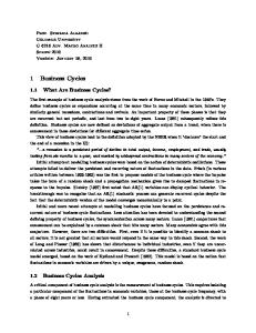
Further, in the general equilibrium of a convex economy, letting β be the discount factor of the economy, we have the familiar relationship 1 + αK0α−1 = 1/β. Combining this relationship with (5) and (10) 1−β and letting m = , the production function thus becomes αβ ( mKt if Kt < K ∗ (A), Yt = (11) AKtα if otherwise. Figure 1 contrasts production function (11) with a standard disembodied production function. In the latter, output jumps from Y0 to A × Y0 when technology increases from A0 to A, even without any investment in new capital. The entire production function shifts up. For Ψ-embodied technology, the production function is linear before capital is accumulated to the steady state, K ∗ (A). Beyond this level, Ψ-embodied technology coincides with the production function Y = AK α . Essentially, production function (11) calls for an AK-technology that is linear in capital with a possibly unknown boundary, beyond which output is concave in capital.

3

Properties of Models with the Ψ-Embodied Technology

The previous section has shown that under certain assumptions of the embodiment function, the production function introduced in our model combines an AK technology and a Cobb-Douglas technology, each applicable within a certain range of (new) capital stock. Though much work has been done studying the properties of the AK models (see, for example, Jones 1995 and McGrattan 1998), to the best of our knowledge, relatively little is known about the properties of such models when the AK technology is applicable to only a certain range of capital stock. This section helps bridge this gap and examines properties of the model that features Ψ-embodied technology and information structure introduced in the previous section.

6

3.1

The Deterministic Case

For expositional purposes, we begin with studying the simplest model where there is no uncertainty about the magnitude of the technological advance and the production function is given by (11). Retaining the assumption of no depreciation and the initial capital stock is at the stead state with respect to the pre-shock level of technology, the social planner’s problem can be written as

max {Ct }

∞ X

β t U (Ct )

(12)

t=0

subject to the resources constraint Ct + It = Yt , the capital accumulation equation (4), and the production function (11). We assume CRRA preferences, such that U (Ct ) = Ct1−σ /1 − σ. In a canonical AK model like Yt = mKt , ∀Kt , we have the familiar balanced growth results—K, C, I, and Y all grow at the same constant rate. In our model, however, output is linear in capital only if Kt < K ∗ (A). Because K ∗ (A) is the steady state level of capital for technology level, A, under production function Y = AKtα , the social planner wants to accumulate exactly K ∗ (A) amount of capital and nothing more than that. Like in a canonical AK model, the first order condition (FOC) requires the marginal utility, hence consumption, to grow at a constant rate as long as the linear technology is applicable, i.e., ¶ µ αβ + 1 − β Ct+1 σ = β(1 + m) = if Kt < K ∗ (A). Ct α

(13)

However, K, and accordingly, Y and I, generally does not grow at the same rate as C does. Indeed, capital stock does not grow even at a constant rate except for some knife-edge levels of A. Appendix A illustrates the variable growth rate in a stylized three-period model of an economy with logarithm preference.

3.2

A Ψ-embodied Technology Model with CRRA Preferences and Pareto-Distributed Shocks

Perhaps somewhat surprisingly, the balanced growth results apply to a Ψ-embodied technology model with unobserved magnitude of technological advances that follows a certain class of probabilistic distribution. In each period in this model, the social planner will find himself in one of the two regimes—the linear regime if Y = mK, or the concave regime if Y = AK α . Learning continues in the linear regime and the magnitude of the underlying technological advance is revealed in the concave regime. Consumption in the linear regime is a decision variable, whereas all output will be consumed in the concave 7

regime, i.e., C = AK α .3 The social planner optimizes the following objective function max E0 {Ct }

∞ X

β t U (Ct ),

t=0

subject to the capital accumulation function (4), the production function (11), and the information structure (6). As Zeira (1987) noted, because all relevant conditional probabilities in future periods can be computed at t = 0, the optimization problem can be written in the more compact form Z ∞ Z Ψt+1 ∞ ∞ X X β t+1 t α max β U (Ct ) φ(A) dA + U (AKt+1 )φ(A) dA, 1 − β Ψt {Kt }t≥1 Ψt t=0

(14)

t=0

where we slightly abuse the notation and use Ct to denote the level of consumption in the linear regime. The level of consumption in the concave regime is written out explicitly as AK α . In the linear regime, Ct = (1 + m)Kt − Kt+1 . Substituting this relationship into (14) and using the Leibniz’s rule repeatedly, we have the following FOC for Kt+1 : © ª U 0 (Ct ) [1 − Φ(Ψt )] = β (1 + m)U 0 (Ct+1 ) [1 − Φ(Ψt+1 )] − U (Ct+1 )φ(Ψt+1 )Ψ0t+1 ·Z Ψt+1 ¸ β α−1 0 α α + αAKt+1 U (AKt+1 )φ(A) dA + U (Ψt+1 Kt+1 )φ(Ψt+1 )Ψ0t+1 1 − β Ψt −

β2 α U (Ψt+1 Kt+2 )φ(Ψt+1 )Ψ0t+1 1−β

(15)

d Ψ(Kt+1 ). Despite its messy appearance, each term of dKt+1 the FOC above has its intuitive economic interpretation. Divide both side by 1 − Φ(Ψt ), the left hand where Ψ0t+1 is the shorthand notation for

side of equation (16) is the marginal utility of consumption in time t, the first row of the right hand side terms is the probability weighted marginal utility in time t + 1 if the production technology stays linear in capital, taking into account the reduction of this probability caused by the marginal investment. Similarly, the second row of the FOC shows the probability weighted marginal utility if the production technology is concave in capital for K = Kt+1 , taking into account the increase of this probability due to the marginal investment. Finally, the last term of the FOC, a trickier one, represents the value of marginal investment made in period t of discovering the true magnitude of A in period t + 1, therefore avoiding making another round of investment that would increase capital to Kt+2 . To have a sharper illustration of the key characteristics of the equilibrium investment dynamics, we assume that investors are able to learn the true magnitude of the technology shock at the borderline when the investment in new capital exactly embodies the new technology, i.e., when A = Ψt+1 .4 Then, 3

Recall that we assume no depreciation in capital. Notice that the production function (11), though not globally differentiable, is continuous, i.e., limK↑K ∗ Y = limK↓K ∗ Y . As long as the magnitude of the technology shock is continuously distributed with no mass on any single point of A, this assumption should be innocuous and do not alter any results quantitatively. 4

8

α = AK α . Several it follows that if Kt+1 exactly embodies A, we have Kt+2 = Kt+1 and Ct+1 = AKt+1 t+2

terms in equation (16) are cancelled out and the FOC can be simplified to R Ψt+1 α−1 0 α )φ(A) dA U (AKt+1 β αAKt+1 1 − Φ(Ψ ) t+1 Ψt U 0 (Ct ) = β(1 + m) U 0 (Ct+1 ) + . 1 − Φ(Ψt ) (1 − β)[1 − Φ(Ψt )]

(16)

To gain further insights of the dynamics implied by the FOC, we now consider a specific parametrizaω tion, assuming CRRA preferences and technology shocks following Pareto distribution: φ(A) = 1+ω A 1 and Φ(A) = ω . After some algebra the FOC (16) can be reorganized to A µ

Ct+1 Ct

¶σ

µ = β(1+m)

Kt+1 Kt

¶(α−1)ω

ω + σ+ω−1

µ

1 m

¶σ µ

Ct+1 Kt+1

¶σ "µ

Kt+1 Kt

¶(α−1)(1−σ)

µ −

Kt+1 Kt

¶(α−1)ω # . (17)

If the economy does have a constant rate, ζ ∗ , of balanced growth on the linear production function Kt+1 Yt+1 It+1 Ct+1 Ct+1 = = = = ζ ∗ , ∀ t if Kt+1 < K ∗ (A), then, the term is also a regime, i.e., Ct Kt Yt It Kt+1 constant and equal to (1 + m) − ζ ∗ . Thus, ζ ∗ solves the following algebraic equation µ ¶ ω 1 + m − ζ σ (α−1)(1−σ−ω) [ζ − 1] − ζ σ−(α−1)ω + β(m + 1) = 0, (18) σ+ω−1 m Table 1 below presents the roots of the equation above for typical values of σ and ω when α = 0.3 and β = 0.96. Table 1: Balanced Growth Rates in Ψ-embodied Technology Models ζ∗

σ=1

σ=2

σ=3

ω = 1.2 ω = 1.5 ω = 1.8

1.065 1.061 1.058

1.038 1.036 1.035

1.027 1.026 1.025

Heuristically, the social planner weighs two types of risk that influence the optimal investment rate from opposite directions. On the one hand, if the economy remains in the linear regime during the next period, the linear production technology would call for a fairly high investment rate. On the other hand, a higher investment rate in the current period will increase the probability of overshooting the optimal capital stock level. Intuitively, the heavier is the tail of the technology shock distribution, the lower is the probability of overshooting. This can be seen in equation (16) as the higher is the [1 − Φ(Ψt+1 )] value , the more weight is put on the marginal utility in the linear regime. For Pareto [1 − Φ(Ψt )] 9

distributions, tail fatness depends on the value of parameter ω. The hazard rate of the distribution, φ(A) ω defined as , is equal to , which increases with ω for any level of A (and decreases with A for 1 − Φ(A) A any value of ω). Therefore, a lower value of ω implies a higher investment and growth rate. Likewise, a higher σ implies the social planner is less willing to give up today’s consumption for tomorrow’s, dζ ∗ leading to a lower investment and growth rate. Indeed, more generally, taking the derivatives and dω ∗ dζ with respect to the implicit function (18), we find the derivatives are negative for typical values of dσ α and β. The canonical AK model can be considered as the special case of the model above, with the distribution of A has a mass equal to one at A = ∞. Such a distribution can be viewed as the Pareto distribution with ω = 0, for which the optimality condition (17) degenerates into (13) and ζ ∗ = 1.933 if σ = 1. Of course, the investment and growth rate is the highest if the social planner does not have to be concerned about overshooting outright.

3.3

A Sufficient Condition for Accelerating Investment

One of the distinct characteristics associated with the IT boom and bust is the decade-long investment boom that ended up with a huge capital overhang and collapse of investment. During the boom, both the level of investment and its share in GDP rose substantially. However, in the economy presented in Section 3.2, investment’s GDP share is a constant. From a theoretical perspective, the IT investment boom motivates us to search for a sufficient condition for accelerating investment such that its share in GDP rises. Examining optimality conditions (16) and (17), we see that when capital stock grows at a constant 1 − Φ(Ψt+1 ) is a constant for Pareto rate ζ ∗ , the term that measures the likelihood of undershooting, 1 − Φ(Ψt ) distributions. If the likelihood of undershooting increases (likelihood of overshooting decreases) with K for any (imposed) fixed growth rate ζ, the optimal investment rate should accelerate over time, eventually causing a capital overhang. When K grows at rate ζ, the level of technology embodied by K increases at rate γ = ζ (1−α) . The technology shock distribution should satisfy ∂ 1 − Φ(γA) > 0, ∂A 1 − Φ(A)

∀A, and γ > 1.

(19)

Applying quotient differentiation rule, it is easy to show that the inequality above is equivalent to the condition below that is more intuitive to interpret, H(γA) 1 < , H(A) γ where H(A) =

∀A, and γ > 1,

φ(A) is the hazard rate function of the distribution. 1 − Φ(A) 10

(20) The condition above

states that if the hazard rate declines more rapidly than the growth of the underlying random variable itself in proportional sense, optimal investment in the linear production regime will accelerate over time. Clearly, the Pareto distribution does not satisfy this condition because for this class of 1 H(γA) distributions, = . It is, however, easy to verify that the truncated Cauchy distribution, H(A) γ 2 φ(A) = , A ∈ (1, ∞), is one example of the distributions that do satisfy (20).5 π[1 + (A − 1)2 ]

3.4

Learning Externality and Model Decentralization

So far we have been studying the properties of the Ψ-embodied technology in the context of a social planner’s optimization. To understand how such a model affect business cycle dynamics, we want to examine whether the equilibrium quantity can be replicated in a decentralized economy. The answer is yes—the social planner’s problem has the same optimal quantity path as the competitive model introduced below—but only when Assumption 4 holds. The equivalent decentralized model can be described as the follows—a representative consumer maximizes the discounted sum of future utility over an infinite time horizon. She owns shares of the firms in the economy, receives dividend payments each period, and can trade the shares to smooth her consumption. The consumer’s problem is max E0

[Ct ,St ]

∞ X

β t U (Ct ),

(21)

t=0

subject to Ct + Pt St = (Pt + Dt )St−1 .

(22)

where St , Dt , and Pt are the share holdings, per-share dividend payment, and the ex-dividend share price at the end of period t, respectively. A unit measure of continuum of identical firms each maximizes the sum of its discounted dividend flow max E0 It

∞ · X

β

t=0

0 (C ) t U 0 (C0 )

tU

¸ Dt ,

(23)

subject to Dt = Yt − It , 5

(24)

The inequality (20) is merely a sufficient, not the necessary, condition for accelerating investment in a setup with no other frictions. As we will show later in the paper, in a more realistically parameterized setup with positive capital depreciation and investment adjustment costs, a technology shock distribution with mildly decreasing hazard rate is able to induce accelerating investment.

11

where output Yt is defined as in (11). ( Yt =

mKt AKtα

if Kt < K ∗ (A), if otherwise.

The information structure is the same as in Section 2.1. It is straightforward to verify that this optimization program has the same set of FOCs as in the social planner’s optimization studied in Section 3.2. Given the initial state of the economy, A0 , K0 , and the unconditional distribution of A, an equilibrium of the decentralized economy is given by a sequence of quantities {Ct , It , Kt , Yt }∞ t=0 and prices ∞ {Pt }∞ t=0 such that given prices {Pt }t=0 , the representative household solves (21); the firm solves (23)

subject to underlying resources constraints. The markets for equity shares and goods clear, such that St = 1 and Ct = Dt ∀t. Recall that Assumption 4 states that a firm can learn only through its own experiments and cannot learn from other firms. This assumption is critical for model decentralization because it shuts off the possible externality learning may generate, ensuring firm i’s investment decision is not a function of firm j’s investment decision. First, the assumption requires that learning takes place at each firm. It is the amount of new capital invested at each firm, not the aggregate amount of new capital in the economy, that determines the productivity of each firm. Second, in a model with ex ante unknown magnitude of technology shocks, learning by investing is risky because the firm is likely to overshoot the optimal level for capital. Without Assumption 4, if one firm can learn about the size of A by observing other firms’ output produced with new capital, this firm will be able to avoid overshooting and invest exactly the optimal amount of capital, thus inducing a free-rider behavior. We defer the discussion of the implied industry dynamics in a model without resorting to Assumption 4 in Section 6.

4

Related Models of Embodied Technology and Learning

Figure 2 illustrates how the model of Ψ-embodied technology introduced above is different from the canonical models of embodied technology, such as Solow (1959). The dashed line is the productivity path after a technology shock in a model without embodiment. It jumps to A from A0 right after the shock arrives at time t0 . The thin solid curve is the average productivity path in a model of Solow-embodied technology with partially irreversible capital. The average productivity converges to A as old capital is being gradually replaced by the new capital that embodies the latest technology. The thick curve represents the productivity path implied by Ψ-embodied technology. At time t0 , the 12

economy learns about the arrival of a new technology and starts investing in new capital. The economy accumulates a sufficient amount of capital at t1 to pick up all of the new technology. Beyond this point, productivity is equal to A. However, investors do not realize this until they observe that learning is completed at t1 + 1 and their expectations on productivity level between t1 and t1 + 1 exceeds the true magnitude of the underlying technology advance. The contrast between Ψ-embodied and Solow-embodied technology reflects two categories of technological innovation. One type of innovation does require substantial replacement of old capital with new capital, whereas the other type of innovation requires adding new capital to complement with old capital. As a stylized example, consider an automobile company producing cars using manually operated assembly lines. A new technology that controls assembly lines with computers is then introduced to the industry. If the old assembly lines cannot work with the computer system and have to be replaced with new assembly lines, the scenario is best described by a Solow model. If the computer system can be used to operate the old assembly lines, the scenario is consistent with Ψ-embodied technology. In such a scenario, it is the productivity of the producer as a whole (both the assembly lines and the controlling system) that increases. The ex ante unknown limit for new capital to embody new technology introduced here shares the same spirit as Zeira (1987), where output is assumed to be the minimum between capital, K, and an ex ante unknown boundary, K ∗ . Similar models are used in Rob (1991) and Barbarino and Jovanovic (2006) in the context of market capacity expansions. Relative to this class of models, our model allows capital to play a richer set of roles—output continues to rise with capital beyond a critical value, though at a lower rate, as additional capital beyond this level does not embody extra new technology into the production but remains as productive as old capital. Furthermore, the critical value of “productive capital,” a term due to Zeira (1987), instead of being given exogenously like in the existing literature, has a rather intuitive and articulated interpretation in our model. Finally, we study the model in a dynamic general equilibrium framework, instead of a partial equilibrium model at the industry or firm level. In our model, learning contributes to prolonging the investment and output boom and endogenously induces overinvestment and a recession. Our proposed learning mechanism is closely related to the literature often referred to as “Bayesian learning by doing.” For example Aghion, Bolton, Harris, and Jullien (1991) study the problem of optimal learning through sequential experimentations. In an application of the theory, Aghion, Bolton, and Jullien (1987) investigate experimental price setting by a monopolist facing demand uncertainty. Learning effects’ potential of generating asymmetries in 13

business cycles has long been appreciated. For example, recently, Van Nieuwerburgh and Veldkamp (2006) study a model where agents cannot tell whether high output is due to better technology or lucky shocks and learning is modelled as a Baysian filter. Economic activities are dense before the business cycle peaks, generating more information that facilitates faster learning and induces an abrupt recession when a negative shock hits. In contrast, at the beginning of the recovery, sluggish economic activities hinder learning and prolong the recovery process.6 Our model is also related to Pastor and Veronesi (2009), who allow for uncertainty about average productivity of new technology and learning about the productivity before large scale adoption of the new technology. In another recent strand of literature, various authors have introduced “news shocks” to the real business cycle models. Like the shocks studied in this paper, such “news shocks” do not immediately change the current production technology but may alter the current economic activities. Beaudry and Portier (2004) revitalize the idea of Pigou (1926) and show that an upward-biased expectation of future productivity growth will lead to an expansion. In a similar spirit, Jaimovich and Rebelo (2009, p.1115) argue that “recessions are driven not by bad shocks today but by lackluster news about the future.” These models do not model learning explicitly. However, allowing for learning may potentially limit the severity of recessions in these models. Should the agents be able to gradually collect additional more accurate information and accordingly revise their expectations about future productivity growth as the boom lasts, they will be less likely surprised by the “lackluster news.”

5

Numerical Examples

This section solves a parameterized model of Ψ-embodied technology and learning in a dynamic general equilibrium setup. The goal of the exercise is to study the following questions. First, can such a model endogenously generate an accelerating investment path? Second, how is investment growth related to the tail properties of the technology shock distribution? Third, does the model present a strong propagation mechanism that allows the economy to have long-lasting reactions to technology shocks? And finally, does the model have the ability of creating endogenous recessions without assorting to real negative shocks? Because we do not calibrate certain key parameters (such as the parameters of technology shock distribution) to match the data, our simulation results are meant to be suggestive and qualitative. To better isolate and highlight the effects of embodied technology and learning on investments, we 6

Also, see Van Nieuwerburgh and Veldkamp (2006) for a concise survey of the literature on the relationship between learning and asymmetry.

14

choose to keep labor supply and demand out of the picture for the current paper and leave it as a subject for future research. Section 3.4 shows that a competitive economy has the same equilibrium quantity path as in a centralized social-planner economy. The latter is more convenient to solve for computationally. Therefore, the model we simulate here is similar to the one we introduced in Section 3.2. The two alternations we made to the numerical model include: first, we allow for asymmetric capital adjustment costs to reflect partial irreversibility of installed capital, which is a fairly standard assumption in the investment dynamics literature (for example, Hall 2001). We did not introduce such an assumption heretofore in order to make the model as analytically tractable as possible. Second, to have a plausible investment share in GDP, we relax the assumption of zero depreciation. However, to keep the model tractable, we assume that the depreciation rates of new and old capital are the same and that the economy simply replenishes the depreciated old capital, i.e., Kold,t ≡ K0 , so that all net investment remains being made in new capital. Specifically, the social planner solves max E {Ct }

∞ X

β t U (Ct )

t=0

subject to the production function (11), the information updating process (6), the capital accumulation equation, and related resources constraints. Deviating from the previous models, we assume there is a positive capital depreciation rate, δ, and capital adjustment costs, Θ. The capital accumulation equation and resources constraints become Kt+1 = (1 − δ)Kt + It ,

(25)

Ct + It + Θt = Yt .

(26)

and

We use the typical parameter values in the business cycles literature and set α = 0.3, annual discount factor β = 0.96, CRRA coefficient σ = 2, and annual depreciation rate δ = 0.1. The parameters and functional form of capital adjustment cost are chosen following Hall (2001). µ ¶ µ ¶ θ+ Kt+1 − Kt 2 θ− Kt+1 − Kt 2 Θt = × P(Kt+1 − Kt ) + × [1 − P(Kt+1 − Kt )], (27) 2 Kt 2 Kt where P is an indicator function such that P(Kt+1 − Kt ) = 1 if Kt+1 − Kt ≥ 0 and P(Kt+1 − Kt ) = 0 if Kt+1 − Kt < 0. θ+ and θ− are the parameters of adjustment costs for positive and negative net investment, respectively. The values of θ+ and θ− are closely related to the persistence of the investment boom. A higher θ+ makes faster investment more costly and a higher θ− makes it more difficult to undo the capital overhang if investment overshoots the optimal level of capital, both prolonging the 15

process of learning and investing. Hall (2001) proposes two values, 2 and 8, as the lower and upper bound for θ+ . We use the geometric average of the two and set θ+ = 4. The parameter θ− is then chosen to be equal to 40, ten times larger than θ+ , to capture the irreversibility of installed capital. What is still left to be chosen is the distribution of the technological innovations. In Section 3 we show that the investment rate and its dynamics is closely related to the hazard rate of the distribution. We examine two technology shock distributions, one with constant hazard rate and one with decreasing hazard rate, to assess how hazard rate affects investment dynamics. We show that in a realistically parameterized model even a distribution the hazard rate of which does not decline as rapidly as required in (20) can induce persistent and accelerating investment. First, normalizing the pre-shock level of productivity A0 = 1, we assume ² = A − A0 = A − 1 follows an exponential distribution, φ(²) = λe−λ² . The hazard rate of the distribution is constant and is equal to λ, which we set equal to 25, giving us a mean of ² equal to 0.04.7 Figure 3 illustrates the impulse-response dynamics of the economy after a new technology arrives.8 The magnitude of this technology shock is equal to 0.2, which is close to the cumulative productivity gain during the 1990s. The upper-left panel shows the conditional expectation of the magnitude of the technology shock. We see that right after the shock arrives, the expectation is simply equal to the unconditional mean, 0.04. In the subsequent periods learning-by-investing continuously pushes up the conditional expectation of ² until investment overshoots the optimal level of capital. In the period right before overshooting takes place, the conditional expectation of ² is equal to 0.24, higher than the true value of the shock. After overshooting, the true value of the shock is revealed. In this setup, we find that investment finally overshoots in the tenth year after the arrival of the new technology. While the economy remains in the learning regime, it also experiences a persistent boom of investment and output. The middle-left panel shows that in the nine consecutive years during which investment has been increasing since the innovation the annual investment growth rate is 3.0 percent and the cumulative growth is 28.5 percent. In the tenth year, when it is learned that capital stock has overshot, investment is reduced dramatically by more than 20 percent. The output dynamics are shown in the bottom-left panel. Output enjoys an equally long-lasting boom before the arrival of an 7

The technology advances considered in this paper are the general purpose technologies (GPT). Such innovations are not expected to take place in every single year. Rather, it arrives once in a long period. The postwar data suggest that, measured by the Solow residuals, the average annual growth of TFP is 0.79 percent. After controlling for the variations in capital utilization and nonconstant returns to scale, Basu, Fernald, and Kimball (2004) report that the “purified” residuals increase on average 0.35 percent annually. Suppose a GPT innovation arrives once in each decade and all productivity increases are due to GPT innovation, the mean of ² should then be between 3.6 and 8.2 percent. We choose the mean of ² closer to the lower bound, acknowledging that not all TFP growth was caused by GPT innovations. 8 Appendix B describes the details of computation.

16

endogenous recession. During the learning phase, output grows at an average annual rate of about 3.0 percent, about the same as the investment. The collapse of the investment also ends the output boom. We see output abruptly becomes flat, though its level does not decrease much in absolute terms. Because the underlying technology innovation distribution has a constant hazard rate, the optimal investment rate as a share of GDP stays flat. In contrast, the NIPA data suggest that the share of private fixed investment increased by almost 30 percent during the 1990s. The consumption dynamics, in the middle-right panel, largely replicate those of the output before the overshooting occurs. It is interesting to observe that at the onset of overshooting consumption increases noticeably because while investment collapsed output does not change much. The counter cyclicality in consumption is consistent with what we observed from the recession after the IT bubble bursted. In the two years following the business cycle peak, the cumulative real GDP growth was only 2.6 percent, whereas the cumulative real consumption growth was almost 5.7 percent. As noted above, the size of capital adjustment costs has a quantitatively important effect on the persistence of the boom. Adopting the lower values in Hall (2001)—θ+ = 2 and θ− = 20—and redoing the exercise, we find that the investment levels are almost 10 percent higher than those in figure 3 before overshooting. Consequently, the boom period shortens to only seven years. Moreover, in such a scenario, the economy overshoots by a larger amount of new capital, making the investment collapse and recession more pronounced. Now, we experiment with an alternative specification for the distribution of technology shocks that has a (mildly) decreasing hazard rate. Assume that the PDF of ² is ξλ1 e−λ1 ² + (1 − ξ)λ2 e−λ2 ² and λ1 < λ2 , a weighted average of two exponential distributions. Unlike the standard exponential distribution that has a constant hazard rate, the hazard rate of this distribution decreases from λ2 to λ1 as ² increase from zero to ∞. We choose the parameters λ1 , λ2 , and ξ to make this distribution have the same mean as the previous one. Figure 4 illustrates how the economy evolves after a shock of ² = 0.2 in this setup. In contrast to the previous case, the conditional expectation of ² increases much more rapidly. Within eight years, it jumps from 0.04, the unconditional mean, to near 0.4 before the economy overshoots. The more rapidly revised belief induces an acceleration in investment. On average, investment grows at an annual rate of 5.5 percent, while its share in GDP increases from 27.2 percent to 31.5 percent.9 Another important distinction in this example relative to the one with constant hazard rate 9

The equilibrium share of investment is higher in our model than in the NIPA, partly due to the assumption of δ = 0.1, which can be too high for many types of capital other than software and equipment in the economy.

17

is that the recession is more pronounced here because the economy has overshot by a larger amount and has to disinvest more capital overhang. Finally, as shown in the bottom-right panels in figure 3 and 4, the model with either of the two distributions implies high levels of (shadow) interest rate over the learning regime. This is because during this period the marginal product of capital, hence the incentive to invest, is very high, depressing the current level of consumption and boosting the expected growth rate of consumption. One counterfactual implication of the model’s shadow interest rate dynamics is that the implied firm’s value would crash at the arrival of new technology and subsequently recover while the learning process is going on.10

6

Concluding Remarks

We propose a novel model of embodied technology. In this model, new technology is embodied in new capital and brings higher productivity for capital of all vintages. Before the full potential of the new technology is reached, the more new capital is invested, the higher is the realized productivity level. Because investors do not know the exact magnitude of the technological innovation, they have to learn it by sequentially investing in new capital. Restricting the model to have the same long-run steady state as the neoclassical growth model without embodied technology, we show that the model can be represented as an AK-production function with an unknown boundary, beyond which output is concave in capital. We show that, with CRRA preferences, the economy enjoys a constant balanced growth while it is in the learning regime if the technological innovations are believed to be drawn from a Pareto distribution. Further, we present a closed-form sufficient condition for accelerating investment and capital overhang, the characteristic observations from the IT boom and bust. The model features a long lasting boom after one sufficiently large technology shock and induces endogenous recessions without evoking any negative shocks. We further argue that it is efficient, ex ante, to allow for the possibilities of such recessions, although they are ex post costly. Numerical results show that a single large technology innovation can induce a boom lasting nearly a decade. In addition, the model is able to generate fairly robust consumption growth during the recession, a phenomenon of the 2001 recession that is hard to be explained in a canonical equilibrium business cycle model. 10

Our model is a closed economy model where every dollar of increase in investment is at the cost of cutting contemporaneous consumption, which in turn raises the expected consumption growth and real interest rate. During the 1990s, especially the later part of the decade, large amounts of foreign capital flowed in and helped keep the interest rate low. The firm value dynamics implied by the Ψ−embodied technology and learning can potentially be more consistent with the data in an open economy setup.

18

Although many of the empirical motivations of the paper are drawn from the IT boom and bust, similar business cycle dynamics existed in many other episodes in history. Jovanovic and Rousseau (2005) document that the share of total power generated by electricity increased sharply between 1900 and 1929, suggesting an investment boom in the electricity industries. The growth of electric power share slowed down abruptly in 1929, the first year of the Great Depression. The electricity expansion never returned to its previous strength, even after the end of the depression. Similar expansions and contractions are documented in the studies of canal and railroad industries in the 19th century. Canal building boomed after the invention of steamboats. Atack and Passell (1994) find that more than 4,000 miles of canal had been completed by the year 1860. However, many of these canals did not live up to the expectations of their promoters and many of these projects eventually turned out to be financial failures. Later in the same century, the railroad expansion shared a similar fate. Thousands of miles of railroad were built and left unused or under used, a phenomenon described by Schumpeter (1949) as constructions “ahead of demand.” Fogel’s investigation (1964) found that the ex post return in the railroad industry in the early 1870s turned out to be too low to attract capital. Overall, the steamboat, the railroad, and electricity all contributed to productivity increases to a great extent, but investment eventually overshot by a large scale. Our ongoing research focuses on relaxing the “learning from yourself” assumption. Allowing for “learning from others” will not only make the model more realistic but also let us able to study interesting industrial dynamics, such as the emergence of technology leaders. Our conjecture is that a subgame perfect equilibrium can arise in such an economy. At the equilibrium, there will be a fraction of firms (technology leaders) that choose to bear the risk of overshooting and invest in new capital. The remainder firms (followers) will wait until the leaders have revealed the magnitude of the technological advance and invest the optimal amount of new capital. The leaders will have a technology competitive edge over the followers, compensating the risk of overshooting. Most interestingly, the fraction of leader firms is endogenously determined, which depends on, among other factors, the demand elasticity and hazard rate of the technology shock distributions.

A

A Three-period Example

Using a stylized three-period model, we illustrate that if the AK technology applies only to a certain range of capital, beyond which output is a concave function of capital, the equilibrium does not call for a balanced growth. In particular, although consumption grows at a constant rate, capital, investment and output does not. We analyze a three-period model because it is the simplest set up 19

that allows us to illustrate the divergence between consumption and capital growth rate. Generically, the optimal number of periods for capital accumulation depends on the magnitude of the shock and should be determined endogenously. For any such optimal number of periods, the results of constant consumption growth and varying rates of investment, capital and output growth hold. max Log(C0 ) + βLog(C1 ) + β 2 Log(C2 )

C0 ,C1 ,C2

subject to Ct + I t = Y t ,

Yt = Kt ,

Kt+1 = Kt + It t = 0, 1, 2,

and K3 = K ∗ Where we further simplify the notation somewhat and set the production function to Yt = Kt , rather than Yt = mKt , as in (11). At the equilibrium, consumption grows at a constant rate 2β, with 2 ∗ 2K0 − K ∗ /4 2 C . In contrast, I = (β + β + 1)K0 + K /4 , I = , C = 2βC and C = 4β C0 = 1 0 2 0 0 1 β2 + β + 1 β2 + β + 1 ∗ 2 ∗ 2 (β − 1)2βK0 + (1 + 2β)K /4 (2β + β + 1)K /2 − 4β K0 , I2 = . Clearly, investment, hence capital 2 β +β+1 β2 + β + 1 and output, does not grow at the same constant rate unless K ∗ takes some knife-edge value.

B

Computation Methods

We use the value function iteration technique over a discrete grid to solve the model. The social planner’s value function can be written as ½ ¾ Z Ψt+1 1 V (Kt ) = max U (Ct ) + β[1 − Φ(Ψt+1 )] × V (Kt+1 ) + W (Kt+1 , A)φ(A) dA , Ct [1 − Φ(Ψt )] Ψt where W (Kt+1 , A) = max {Iτ }

∞ X

β τ −t U (A Kτα − Iτ − Θτ ) .

(28)

τ =t+1

is the post-learning value function if the magnitude of the technological innovation is revealed to be equal to A. We discretize the technology shock distribution with N points, and each point has weight equal to

1 N.

Depending on the shape of the distribution, N may have to be rather large to capture

the tail properties. Meanwhile I discretize the state variable, K. It is straightforward to compute the post-learning value function W (K, A) by iterating W (K, A) alone because it does not involve V (K). [1 − Φ(Ψt+1 )] We then compute for all possible pairs Kt+1 > Kt on the K grid. Finally, we iterate [1 − Φ(Ψt )] the entire value function V (K) until the gap is smaller than 0.0001. 20

References [1] Aghion, Philippe, Patrick Bolton, and Bruno Jullien (1987), “Learning Through Price Experimentation by a Monopolist Facing Unknown Demand”, MIT Working Paper. [2] Aghion, Philippe, Patrick Bolton, Christopher Harris, and Bruno Jullien (1991), “Optimal Learning by Experimentation”, Review of Economic Studies, vol. 58 (June), pp. 621-54. [3] Atack, Jeremy and Peter Passell (1994) “A New Economic View of American History from Colonial Times to 1940”, New York: W.W. Norton & Company. [4] Barbarino, Alessandro and Boyan Jovanovic (2007), “Shakeouts and Market Crashes”, International Economic Review, vol. 48 (May), pp. 395-420. [5] Basu, Susanto, John Fernald and Miles Kimball (2006). “Are Technology Improvements Contractionary?”, American Economic Review, vol. 96 (December), pp. 1418-48. [6] Beaudry, Paul and Franck Portier (2004), “An Exploration into Pigou’s Theory of Cycles”, Journal of Monetary Economics, vol. 51 (September), pp. 1183-216. [7] Cogley, Timothy and James M. Nason (1995) “Output Dynamics in Real-Business-Cycle Models”, American Economic Review, vol. 85 (June), pp. 492-511. [8] Fogel, Robert (1964), “The Union Pacific Railroad: A Case in Premature Enterprise”, Baltimore: Johns Hopkins University Press. [9] Hall, Robert (2001), “The Stock Market and Capital Accumulation”, American Economic Review, vol. 91 December, pp. 1185-202. [10] Jaimovich, Nir and Sergio Rebelo (2009), “Can News About the Future Drive the Business Cycle?” American Economic Review, vol. 99 (December), pp. 107-118. [11] Jones, Charles I. (1995), “Time series tests of endogenous growth models,” Quarterly Journal of Economics vol. 110 (May), pp. 495525. [12] Jovanovic, Boyan and Peter Rousseau (2005), “General Purpose Technology”, chapter in the Handbook of Economic Growth, vol.1, part 2, pp. 1181-224. [13] McGrattan, Ellen R. (1998), “A Defense of AK Growth Models,” Fedearl Reserve Bank of Minneapolis Quarterly Review, vol. 22, pp. 13 - 27. [14] Van Nieuwerburgh, Stijn and Laura Veldkamp (2006), “Learning Asymmetries in Real Business Cycles”, Journal of Monetary Economics, vol. 53 (May), pp. 753-72. 21

[15] Pastor, Lubos and Pietro Vironesi (2009) “Technological Revolutions and Stock Prices,” American Economic Review, vol. 99, September pp. 1451 1463. [16] Pigou, Arthur Cecil (1926), “Industrial Fluctuations”, New York: A.M. Kelly. [17] Rob, Rafael (1991), “Learning and Capacity Expansion under Demand Uncertainty”, Review of Economic Studies, vol. 58 (June), pp. 655-75. [18] Schumpeter, Joseph (1949), “The Theory of Economic Development”. Cambridge: Harvard University Press. [19] Solow, Robert (1959), “Investment and Technological Progress”, In Kenneth Arrow, Samuel Karlin and Patrick Suppes, eds., Mathematical Methods in the Social Sciences, Stanford, CA: Stanford University Press, pp. 89-104. [20] Zeira, Joseph (1987), “Investment as a Process of Search”, Journal of Political Economy, vol. 95 (February), pp. 204-10.

22

Y

Y = (K0)

-1

* K Y= AK

Y= K

A*Y0

Y0

K0

K*(A)

K

Figure 1: Comparison of Output Changes between the Standard Cobb-Douglas and Ψ-Embodied Technology

23

Expected Productivity

Productivity

A

A0

0

t0

t1

t1+1

t

Disembodied Technology, Model in this Paper, -embodied Technology Solow-Embodied Technology.

Figure 2: Productivity Changes in Disembodied, Solow-Embodied, and Ψ-Embodied Technology Models

24

0.4 0.3 0.2 0.1 0

0

5 10 15 year after the technology shock Investment

20

investment share in GDP

conditional expectation about ε

ε expectation

Investment Share

0.3 0.25 0.2 0.15

consumption

investment

2

1.5

1

0

5 10 15 year after the technology shock Output

5 10 15 year after the technology shock Consumption

20

0

5 10 15 year after the technology shock Interest Rate

20

0

5 10 15 year after the technology shock

20

1.4 1.2 1 0.8

20

0

0.4 interest rate

output

1.4 1.2 1 0

5 10 15 year after the technology shock

0.3 0.2 0.1 0

20

Figure 3: Impulse Response of a Constant Hazard Rate ² Distribution

25

0.4 0.3 0.2 0.1 0

0

5 10 15 year after the technology shock Investment

20

investment share in GDP

conditional expectation about ε

ε expectation

Investment Share

0.3 0.25 0.2 0.15

consumption

investment

2

1.5

1

0

5 10 15 year after the technology shock Output

5 10 15 year after the technology shock Consumption

20

0

5 10 15 year after the technology shock Interest Rate

20

0

5 10 15 year after the technology shock

20

1.4 1.2 1 0.8

20

0

0.4 interest rate

output

1.4 1.2 1 0

5 10 15 year after the technology shock

0.3 0.2 0.1 0

20

Figure 4: Impulse Response of a Decreasing Hazard Rate ² Distribution

26