Learning and Approximation of Chaotic Time Series Using Wavelet-Networks V. Alarcon-Aquino, E. S. García-Treviño, R. Rosas-Romero, L.G. Guerrero-Ojeda Departamento de Ingenieria Electrónica Universidad de las Américas Puebla, Sta. Catarina Mártir. Cholula, Puebla. C.P. 72820. MEXICO E-mail:
[email protected],
[email protected] Abstract This paper presents a wavelet neural-network for learning and approximation of chaotic time series. Wavelet networks are a class of neural network that take advantage of good localization and approximation properties of multiresolution analysis. This kind of network use wavelets as activation functions in the hidden layer and a noniterative method is used for its learning. Comparisons are made between a wavelet network, tested with two different wavelets, and the typical feed-forward networks trained with the backpropagation algorithm. The results reported in this paper show that wavelet networks have better approximation properties than its similar backpropagation networks. Keywords: wavelet networks, wavelets, chaos theory, back-propagation networks, approximation theory, multiresolution analysis.
1. Introduction Wavelet neural networks are a novel powerful class of neural networks that incorporate the most important advantages of multiresolution analysis introduced by Mallat in 1989 [6]. These networks preserve all the features of common neural networks, but in addition, have rigorous mathematical foundations. In wavelet networks, the activation functions have good localization properties; this important characteristic allows hierarchical and multiresolution learning as well as transparent design of the network. Wavelets are a new family of basis functions that combine powerful properties such as orthogonality, compact support, localization in time
and frequency, and fast algorithms. Wavelets have generated a tremendous interest in both theoretical and applied areas, especially over the past few years [10]. Wavelet based methods have been used for approximation theory, pattern recognition, compression, numerical analysis, computer science, electrical engineering, physics etc. Wavelet networks are a class of neural networks that employ wavelets as activation functions. These have been recently researched as an alternative approach to the traditional neural networks with sigmoidal activation functions. Wavelet networks have attracted great interest, because of their advantages over other networks schemes (see e.g., [9]). There are two main research groups that combine wavelet theory and neural networks, both with a comprehensive framework. The first is based on the work of Zhang and Benveniste [8] [11], that introduces a (1+½) layer neural network based on wavelets, but their approach is still using a type of backpropagation algorithm to train de network. The second is based on the work initiated by Bakshi and Stephanopoulos [7], in which wavelets are used in a structure similar to radial basis function networks, but a non-iterative and hierarchical method is used for learning [5]. We based this work on the second approach, following the concept of locally supported basis functions such as radial basis function networks and from wavelet decomposition in signal processing. Function approximation involves estimating the underlying relationship from a given finite inputoutput data set, and it has been the fundamental problem for a variety of applications in pattern classification, data mining, signal reconstruction, and system identification [4]. Recently, feedforward neural networks such as multilayer perceptrons and radial basis function networks
have been widely used as an alternative approach to function approximation since they provide a generic black-box functional representation. Furthermore, these networks have shown to be capable of approximating any continuous function defined on a compact set in ‘8 , where ‘ denotes real numbers, with arbitrary accuracy. In this work we show the powerful and the abilities of this kind of networks, making approximation of time series. Particularly, we present wavelet networks applied to the approximation of chaotic time series. For this purpose comparisons are made between a wavelet network, tested with two different wavelets, and the typical feed-forward networks trained with the backpropagation algorithm [3]. The results reported in this work show clearly that wavelet networks have better approximation properties than its similar backpropagation networks. The reason for that is the firm theoretical foundations of wavelet networks, that combine, the mathematical methods and tools of multiresolution analysis with the neural network framework. The remainder of this paper is organized as follows. Section 2 briefly reviews wavelet theory. Section 3 describes the wavelet network structure. In Section 4 chaotic time series are presented. In Section 5 comparisons between wavelet networks and back-propagation networks are made and discussed. Finally, Section 5 presents the conclusions of this work.
2. Review of wavelet theory Wavelet transforms involve representing a general function in terms of simple, fixed building blocks at different scales and positions. These building blocks are generated from a single fixed function called mother wavelet by translation and dilation operations. The continuous wavelet transform considers a family <+ß, ÐBÑ œ
" B, < ß Èl+l Œ +
(1)
where + − ‘ ß , − ‘, with + Á !, and <Ð † Ñ satisfies the admissibility condition. For discrete wavelets the scale (or dilation) and translation parameters in (1) are chosen such that at level 7 the wavelet +!7 <Ð+!7 BÑ is +!7 times the width of <ÐBÑ. That is, the scale parameter Ö+ œ +!7 À 7 − ™× and the translation parameter Ö, œ 5,! +!7 À 7ß 5 − ™×. This family of wavelets is thus given by
<7ß5 aBb œ +!
7Î#
(2)
so the discrete version of wavelet transform is .7ß5 œ Ø1ÐBÑß <7ß5 ÐBÑÙ
7Î#
œ +!
' _ 1ÐBÑ
(3)
Ø † ß † Ù denotes the P# -inner product. To recover 1ÐBÑ from the coefficients Ö.7ß5 ×, the following stability condition should exist [2], Em1ÐBÑm# Ÿ " "l 1ÐBÑß <7ß5 ÐBÑ¡l# Ÿ Fm1ÐBÑm# ß 7−™ 5−™
(4) with E ! and F _ for all signals 1ÐBÑ in P# Ð‘Ñ denoting the frame bounds. These frame bounds can be computed from +! , ,! and <ÐBÑ [12]. The reconstruction formula is thus given by 1ÐBÑ ¸
# " " 1ÐBÑß <7ß5 ÐBÑ¡<7ß5 ÐBÑÞ E F 7−™ 5−™ (5)
Note that the closer E and F , the more accurate the reconstruction. When E œ F œ ", the family of wavelets then forms an orthonormal basis [12]. 2.1 Orthonormal bases and multiresolution analysis The mother wavelet function <ÐBÑ, scaling +! and translation ,! parameters are specifically chosen such that <4ß8 ÐBÑ constitute orthonormal bases for P# Ð‘Ñ [6], [12]. To form orthonormal bases with good time-frequency localisation properties, the time-scale parameters Ð,ß +Ñ are sampled on a so-called dyadic grid in the time-scale plane, namely, +! œ # and ,! œ ", [6], [12]Þ Thus, from Eq. (2) substituting these values, we have a family of orthonormal bases, <7ß5 ÐBÑ œ #7Î#
(6)
Using Eq. (3), the orthonormal wavelet transform is thus given by 1ÐBÑß <7ß5 ÐBÑ¡ =
#7Î# '_ 1ÐBÑ<7ß5 a#7 B 5 b.B _
(7)
19 ÐBÑ œ ! -!ß5 9!ß5 ÐBÑ
and the reconstruction formula is obtained from Eq. (5). A formal approach to constructing orthonormal bases is provided by multiresolution analysis (MRA) [6]. The idea of MRA is to write a function 1ÐBÑ as a limit of successive approximations, each of which is a smoother version of 1ÐBÑ. The successive approximations thus correspond to different resolutions [6].
Then, by including the wavelets of the same resolution, a finer approximation is provided,
2.2 Discrete Wavelet Transform: Decomposition and Reconstruction
In general, adding wavelets of a higher resolution to a current approximation, a finer approximation of 1ÐBÑ is obtained,
Since the idea of multiresolution analysis is to write a signal 1ÐBÑ as a limit of successive approximations, the differences between two successive smooth approximations at resolution #7" and # give the detail signal at resolution #7 . In other words, after choosing an initial resolution P, any signal 1ÐBÑ − P# Ð‘Ñ can be expressed as [6], [12]: 1ÐBÑ œ "-Pß5 9Pß5 ÐBÑ " ".7ß5 <7ß5 ÐBÑß _
5−™
1" ÐBÑ œ 19 ÐBÑ ! .!ß5
17" ÐBÑ œ 17 ÐBÑ ! .7ß5 <7ß5 ÐBÑ
_
This process can be continued until the function 1ÐBÑ is re-produced as in equation (8). Figure 1 shows a typical wavenet structure. At each stage of learning, the approximation problem may be expressed as s17 ÐBÑ œ ! -7ß5 )7ß5 ÐBÑ
where
s17 ÐBÑ œ 1ÐBÑ 17 ÐBÑ φ − nodes φ Lk φ Lk
x
ψLk ψ mk
cˆLk cˆLk dˆLk
∑
dˆmk
gˆ
dˆ1k
ψ1k
3. Description of wavelet-networks As stated previously, we based this work on the wavelet network approach introduced by Bakshi and Stephanopoulos [7] in which wavelets are used in a structure similar to radial basis function networks. Equation (8) represents the basic framework for the construction of wave-nets. A wave-net is defined as a one hidden layer network whose basis functions are drawn from a family of orthogonal wavelets [7]. Multiresolution analysis is the framework for its learning. In fact, by incorporating the basis functions at a particular resolution, namely 7=0 here, the first approximation to the desired function is obtained [14],
(13)
5−™
Ð*Ñ
Equations (7) and (9) express that a signal 1ÐBÑ is decomposed in details Ö.7ß5 × and approximations Ö-7ß5 × to form a multiresolution analysis of the signal [6].
(12)
5−™
where the detail or wavelet coefficients Ö.7ß5 × are given by Eq. (7), while the approximation or scaling coefficients Ö-7ß5 × are defined by -7ß5 œ #7Î# '_ 1ÐBÑ97ß5 a#7 B 5 b.B
(11)
5−™
7œP5−™
(8)
(10)
5−™
ψ − nodes
Figure 1. A typical wavenet structure Now, if one considers a practical case of finite discrete sequences of inputs and outputs, the equation (13) leads to where
(14)
s1 œ EG
Ô s1ÐB" Ñ × Ô )" ÐB" Ñ Ö s1ÐB# Ñ Ù Ö ) ÐB Ñ Ù EœÖ " # s1 œ Ö ã ã Õ s1ÐB8 Ñ Ø Õ )" ÐB8 Ñ
ÞÞÞ ÞÞÞ ÞÞÞ
)5 ÐB" Ñ × )5 ÐB# Ñ Ù Ù ã )5 ÐB8 Ñ Ø
Ô -" × Ö- Ù G œÖ #Ù ã Õ -5 Ø
(15)
The least squares solution of (14) is given by G œ ÐÐEX EÑ" EX Ñ1 s œ Es1
(16)
where E+ is the pseudo-inverse of matrix E. If data are regularly sampled and the basis functions are orthonormal, !5 )# Ð5Ñ œ " then EX E becomes an identity matrix and equation is simplified to: (17)
G œ EX s1
4. Chaotic time series Chaos is the mathematical term for the behavior of a system that is inherently unpredictable.
Unpredictable phenomena are readily apparent in all areas of life [1]. Many systems in the natural world are now known to exhibit chaos or nonlinear behavior, the complexity of which is so great that they were previously considered random. The unraveling of these systems has been aided by the discovery, mostly in this century, of mathematical expressions that exhibit similar tendencies [2]. In this section, we present briefly the four chaotic time series used in this work (see Figure 2). 4.1 Logistic map It was explored by ecologist and biologist who used it to model population dynamics. It was popularized by Robert May in 1976 as an example of a very simple nonlinear equation being able to produce very complex dynamics. The mathematical equation that describes the logistic map has the form: BÐ> "Ñ œ +BÐ>ÑÐ" BÐ>ÑÑ (18)
time
time
1
2
1
0.6
amplitude
amplitude
0.8
0.4
-1
0.2 0
0
0
10
20
30
40
-2
50
0
10
20
20
20
10
10
0
-10
-20
30
40
50
30
40
50
(b)
amplitude
amplitude
(a)
0
-10
0
10
20
30 (c)
40
50
-20
0
10
20 (d)
Figure 2. Chaotic series: (a) Logistic map, (b) Henon attractor, (c) Lorenz attractor, (d) Rossler attractor.
where + œ %, and BÐ!Ñ œ !Þ!!!"!%.
the
initial
condition
4.2 Rossler attractor It was introduced for Otto Rossler and arose from work in chemical kinetics. The system is described with 3 coupled non-linear differential equations: .B (19) .> œ C D .C .> œ B +C .D œ , DÐB -Ñ .> where + œ !Þ"&ß , œ !Þ#!ß - œ "!. 4.3 Lorenz attractor It was introduced by E. N. Lorenz, in 1963. It was derived from a simplified model of atmospheric interactions. The system is most commonly expressed as 3 coupled non-linear differential equations: .B (20) .> œ +ÐC BÑ .C œ BÐ, DÑ C .> .D .> œ BC -DÑ where + œ "!ß , œ #)ß - œ )Î$. 4.4 Hénon Attractor It was introduced by M, Hénon in 1976, and was derived from a study of chaotic functions trajectories. .B # (21) .> œ + ,C B .C œ B .> where + œ "Þ%ß , œ !Þ$ . The chaotic series described previously are considered for this work because they illustrate how the complex behavior can easily be produced by simple equations with non-linear elements and feedback. Figure 2 shows these four chaotic time series plotted for the first 50 samples.
5. Simulation results This work present wavelet networks applied to the approximation of four of the most known chaotic time series: Logistic Map, Lorenz Attractor, Hénon Attractor, and Rossler Attractor. Particularly, this section presents comparisons
between a wavelet network, tested with two different wavelets, and the typical feed-forward networks trained with the backpropagation algorithm [3]. The last three time series mentioned previously were obtained from [14]. Lorenz attractor was sampled every 0.01 time steps, Rossler and Hénon series every 0.1 time steps. For an appropriate learning, and taking into account the features of the activation functions used by the networks analyzed, the four series were normalized in the range of 0-1. For the basis functions of the wavelet network approach we first test it with orthogonal BattleLemarie wavelet (wavenet(1)) and afterwards with Haar wavelet (wavenet(2)). For the backpropagation network, we use tangent-sigmoidal activation functions, and it was trained with a learning rate of 0.1, the momentum term was set at 0.07, and 5000 iterations. The same architecture was used for BPN and for the wavenetsß that is, 16-1 (one input layer, six hidden units and one output unit). For all series the first 300 samples were used for training and the next 200 samples for testing. Table 1. Simulations results
Approach Wavenet (1) Wavenet (2) BP Approach Wavenet (1) Wavenet (2) BP Approach Wavenet (1) Wavenet (2) BP Approach Wavenet (1) Wavenet (2) BP
Logistic map MSE(training) MSE (testing) 0.001443 0.001201 0.049707 0.050050 0.121968 0.133198 Hénon attractor MSE(training) MSE (testing) 0.065681 0.0797552 0.028381 0.031613 0.074312 0.080172 Lorenz attractor MSE(training) MSE (testing) 0.059465 0.058034 0.060698 0.060266 0.060410 0.062313 Rossler attractor MSE(training) MSE (testing) 0.039531 0.041005 0.041139 0.042490 0.053366 0.055777
As can be seen in Table 1, wavelet networks outperform BPN when using Battle-Lemarie and Haar Wavelets. This is due to the fact that neural networks based on conventional single-resolution schemes cannot learn difficult time series, with
abrupt changes in its behavior; consequently the training process often converge very slowly and the trained network may not generalize well. It is worth noting that the wavenet(1) performs a better approximation than the wavenet(2). This is due to the fact that the Battle-Lemarie wavelet has higher degree of smoothness than the Haar wavelet. A higher degree of smoothness in a wavelet corresponds to better frequency localization [10].
6. Conclusions The results reported in this work show clearly that wavelet networks have better approximation properties than its similar backpropagation networks. The reason for that is the firm theoretical foundations of wavelet networks, that combine, the mathematical methods and tools of multiresolution analysis with the neural network framework. The wavelet selected as basis function for the studied approach play an important role in the approximation process. Generally the selection of the wavelet depends on the kind of function to be approximated. In our particular case, due to the features of time series studied, a wavelet with good high-frequency localization like Battle-Lemarie, showed better approximation results.
7. References: [1] R. L. Devaney, "Chaotic Explosions in Simple Dynamical Systems", The Ubiquity of Chaos, Edited by Saul Krasner. American Association for the Advancement of Science. Washington D. C., U.S.A. 1990 [2] J. Pritchard, "The Chaos CookBook: A practical programming guide", Part of Reed International Books. Oxford. Great Britain. 1992. [3] S. Y. Kung, "Digital Neural Networks", Department of Electrical Engineering, Princeton University, Prentice Hall. New Jersey. U.S.A. 1993. [4] S. Sitharama Iyengar, E.C. Cho, Vir V. Phoha, "Foundations of Wavelet Networks and Applications", Chapman & Hall/CRC. U.S.A. 2002 [5] A. A. Safavi, H. Gunes, J.A. Romagnoli, "On the Learning Algorithms for Wave-Nets", Department of Chemical Engineering, The University of Sydney. Australia. 2002, [6] S. G. Mallat, "A theory for Multiresolution Signal Decomposition: The Wavelet Representation", IEEE
Transactions on Pattern Analysis Intelligence. Vol II. No 7. July 1989
and
Machine
[7] B. R. Bakshi, G.Sthepanopoulos, "Wavelets as Basis Functions for Localized Learning in a Multiresolution Hierarchy", Laboratory for Intelligent Systems in Process Engineering, Department of Chemical Engineering. Massachusetts Institute of Technology, Cambridge, MA 02139, 1992 [8] Q. Zhang, A. Benveniste, "Wavelet Networks", IEEE Transactions on Neural Networks. Vol 3. No 6. July 1992 [9] E. A. Rying, Griff L. Bilbro, and Jye-Chyi Lu. "Focused Local Learning With Wavelet Neural Networks", IEEE Transactions on Neural Networks, Vol. 13, No. 2, March 2002. [10] B. Jawerth, W. Sweldens. "An overview of wavelet based multiresolution analyses", SIAM, 1994. [11] Xeiping Gao, Fen Xiao, Jun Zhang, Chunhong Cao. "Short-term Prediction of Chaotic Time Series by Wavelet Networks", WCICA, Fifth World Congress on Intelligent Control And Automation, 2004. [12] I, Daubechies. "Ten Lectures on Wavelets", New York. SIAM. 1992. [13] A. A. Safavi, J. A.Romagnoli "Application of Wave-nets to Modellling and Optimisation of a Chemical Process" Safavi, A.A. Romagnoli, J.A. Proceedings., IEEE International Conference on Neural Networks, 1995. [14 ] E, R Weeks. http://www.physics.emory.edu/~weeks/