PHYSICAL REVIEW B 76, 045321 共2007兲

Kondo quantum dot coupled to ferromagnetic leads: Numerical renormalization group study M. Sindel,1 L. Borda,1,2 J. Martinek,3,4,5 R. Bulla,6 J. König,7 G. Schön,5 S. Maekawa,3 and J. von Delft1 1Physics

Department, Arnold Sommerfeld Center for Theoretical Physics, and Center for NanoScience, Ludwig-Maximilians-Universität München, 80333 München, Germany 2 Research Group “Theory of Condensed Matter” of the Hungarian Academy of Sciences, TU Budapest, Budapest H-1521, Hungary 3Institute for Materials Research, Tohoku University, Sendai 980-8577, Japan 4Institute of Molecular Physics, Polish Academy of Sciences, 60-179 Poznań, Poland 5Institut für Theoretische Festkörperphysik and DFG-Center for Functional Nanostructures (CFN), Universität Karlsruhe, D-76128 Karlsruhe, Germany 6Theoretische Physik III, Elektronische Korrelationen und Magnetismus, Universität Augsburg, D-86135 Augsburg, Germany 7 Institut für Theoretische Physik III, Ruhr-Universität Bochum, 44780 Bochum, Germany 共Received 18 July 2006; revised manuscript received 3 November 2006; published 18 July 2007兲 We systematically study the influence of ferromagnetic leads on the Kondo resonance in a quantum dot tuned to the local moment regime. We employ Wilson’s numerical renormalization group method, extended to handle leads with a spin asymmetric density of states, to identify the effects of 共i兲 a finite spin polarization in the leads 共at the Fermi surface兲, 共ii兲 a Stoner splitting in the bands 共governed by the band edges兲, and 共iii兲 an arbitrary shape of the lead density of states. For a generic lead density of states, the quantum dot favors being occupied by a particular spin species due to exchange interaction with ferromagnetic leads, leading to suppression and splitting of the Kondo resonance. The application of a magnetic field can compensate this asymmetry, restoring the Kondo effect. We study both the gate voltage dependence 共for a fixed band structure in the leads兲 and the spin polarization dependence 共for fixed gate voltage兲 of this compensation field for various types of bands. Interestingly, we find that the full recovery of the Kondo resonance of a quantum dot in the presence of leads with an energy-dependent density of states is possible not only by an appropriately tuned external magnetic field but also via an appropriately tuned gate voltage. For flat bands, simple formulas for the splitting of the local level as a function of the spin polarization and gate voltage are given. DOI: 10.1103/PhysRevB.76.045321

PACS number共s兲: 72.15.Qm, 75.20.Hr, 72.25.⫺b, 73.23.Hk

I. INTRODUCTION

The interplay between different many-body phenomena, such as superconductivity, ferromagnetism, or the Kondo effect, has recently attracted a lot of experimental and theoretical attention. A recent experiment of Buitelaar et al.1 nicely demonstrated that Kondo correlations compete with superconductivity in the leads. The interplay between Kondo correlations and itinerant electron ferromagnetism in the electrodes has theoretically been intensively studied within the last years,2–9 initially leading to controversial conclusions. For effectively single-level quantum dots 共i.e., dots with a level spacing much bigger than the level broadening ⌫兲, consensus was found that a finite spin asymmetry in the density of states in the leads results 共in general兲 in splitting and suppression of the Kondo resonance. This is due to the spindependent broadening and renormalization of the dot level position induced by spin-dependent quantum charge fluctuations. In terms of the Kondo spin model, it can be treated as an effective exchange interaction between a localized spin on the dot and ferromagnetic leads. Moreover, it was shown that a strong coupling Kondo fixed point with a reduced Kondo temperature can develop6,7 even though the dot is coupled to ferromagnetic leads, given that an external magnetic field6 or electric field7 共gate voltage兲 is tuned appropriately. Obviously, in the limit of fully spin-polarized leads, when only one spin component is present for energies close to the Fermi surface 共half-metallic leads兲, the effective screening of the impurity cannot take place any more and the Kondo reso1098-0121/2007/76共4兲/045321共17兲

nance does not develop. A part of these theoretical predictions have recently been confirmed in an experiment by Pasupathy et al.10 The presence of ferromagnetic leads could also nicely explain the experimental findings of Nygård et al.11 Since the interplay between ferromagnetism and strong correlation effects is one of the important issues in spintronic applications, there are currently many research activities going on in this direction. The goal is to manipulate the magnetization of a local quantum dot 共i.e., its local spin兲 by means of an external parameter, such as an external magnetic field or an electric field 共a gate voltage兲, with high accuracy. This would provide a possible method of writing information in a magnetic memory.12 Since it is extremely difficult to confine a magnetic field such that it only affects the quantum dot under study, it is of big importance to search for alternative possibilities for such a manipulation 共e.g., by means of a local gate voltage, as proposed by the authors13兲. In this paper, we push forward our previous work by performing a systematic analysis on the dependence of physical quantities on different band structure properties. Starting from the simplest case, we add the ingredients of a realistic model one by one, allowing a deeper understanding of the interplay of the Kondo model and itinerant electron ferromagnetism. In this paper, we extend our recent studies carried out in this direction6,7,13 and illustrate the strength of the analytical methods by comparing the results predicted by them to the results obtained by the exact numerical renormalization group 共NRG兲 method.14 While in Refs. 2–9 the dot was attached to ferromagnetic leads with an unrealistic, spin-

045321-1

©2007 The American Physical Society

PHYSICAL REVIEW B 76, 045321 共2007兲

SINDEL et al.

independent, and flat band—with a spin-dependent tunneling amplitude—we generalize this treatment here by allowing for arbitrary density of states 共DOS兲 shapes.13 In particular, we carefully analyze the consequences of typical DOS shapes in the leads on the Kondo resonance. We explain the difference between these shapes and provide simple formulas 共based on perturbative scaling analysis15,16兲 that explain the numerical results analytically. We study both the effect of a finite lead spin polarization and the gate voltage dependence of a single-level quantum dot contacted to ferromagnetic leads with three relevant DOS classes: 共i兲 for flat bands without Stoner splitting, 共ii兲 for flat bands with Stoner splitting and, 共iii兲 for an energy-dependent DOS 共also including Stoner splitting兲. For this sake, we employ an extended version of the NRG method to handle arbitrary shaped bands.17 The article is organized as follows: In Sec. II, we define the model Hamiltonian of the quantum dot coupled to ferromagnetic leads. In Sec. III, we explain details of the Wilson mapping on the semi-infinite chain in the case of the spindependent density of states with arbitrary energy dependence. Using the perturbative scaling analysis, we give prediction for a spin-splitting energy for various band shapes in Sec. IV. In Sec. V, the results for spin-dependent flat DOS are demonstrated, together with the Friedel sum rule analysis. The effect of the Stoner splitting is discussed in Sec. VI, together with comparison to experimental results from Ref. 11 and an arbitrary band structure in Sec. VII. We summarize our findings then in Sec. VIII.

dispersion function ⑀rk␴. Vrk labels the tunneling matrix element between the impurity and lead r, Sz = 共nˆ↑ − nˆ↓兲 / 2, and the last term in Eq. 共1兲 denotes the Zeeman energy due to external magnetic field B acting on the dot spin only. Here, we neglect the effect of an external magnetic field on the leads’ electronic structure, as well as a stray magnetic field from the ferromagnetic leads. The coupling between the dot level and electrons in lead r leads to a broadening and a shift of the level ⑀d, ⑀d →˜⑀d 共where the tilde denotes the renormalized level兲. The energy and spin dependency of the broadening and the shift, determined by the coupling, ⌫r␴共␻兲 = ␲␳r␴共␻兲兩Vr共␻兲兩2, plays the key role in the effects outlined in this paper. Henceforth, we assume Vrk to be real and k independent, Vrk␴ = Vr, and lump all energy and spin dependence of ⌫r␴共␻兲 into the DOS in lead r, ␳r␴共␻兲.18 Without loosing generality, we assume the coupling to be symmetric, VL = VR. Accordingly, by performing a unitary ˆ ˆ = 1 兺 共⑀ simplifies to H transformation,19 H ᐉ ᐉ 2 k␴ Lk␴ † + ⑀Rk␴兲␣sk␴␣sk␴, where ␣sk␴ denotes the proper unitary combination of lead operators which couple to the quantum dot and we dropped the part of the lead Hamiltonian which is decoupled from the dot. With the help of the definitions V ⬅ 冑VL2 + VR2 , ␣k␴ ⬅ ␣sk␴, and ⑀k*␴ ⬅ 21 共⑀Lk␴ + ⑀Rk␴兲, the full Hamiltonian can be cast into a compact form,

II. MODEL: QUANTUM DOT COUPLED TO FERROMAGNETIC LEADS

A. Ferromagnetic leads

We model the problem at hand by means of a single-level dot of energy ⑀d 共tunable via an external gate voltage VG兲 and charging energy U that is coupled to identical, noninteracting leads 共in equilibrium兲 with Fermi energy ␮ = 0. Accordingly, the system is described by the following Anderson impurity model: ˆ +H ˆ , ˆ =H ˆ +H H ᐉ ᐉd d ˆ = ⑀ 兺 nˆ + Unˆ nˆ − BS , H d d ␴ ↑ ↓ z ␴

共1兲

with the lead and the tunneling part of the Hamiltonian ˆ = 兺 ⑀ c† c , H ᐉ rk␴ rk␴ rk␴

共2兲

ˆ = 兺 共V d† c + H.c.兲. H ᐉd rk ␴ rk␴

共3兲

rk␴

rk␴

Here, crk␴ and d␴ 共nˆ␴ = d␴† d␴兲 are the Fermi operators for electrons with momentum k and spin ␴ in lead r 共r = L / R兲 and in the dot, respectively. The spin-dependent dispersion in lead r, parametrized by ⑀rk␴, reflects the spin-dependent DOS, ␳r␴共␻兲 = 兺k␦共␻ − ⑀rk␴兲, in lead r; all information about energy and spin dependency in lead r is contained in the

ˆ , ˆ = 兺 ⑀* ␣† ␣ + 兺 V共d† ␣ + H.c.兲 + H H d k␴ k␴ k␴ ␴ k␴ k␴

k␴

共4兲

ˆ as given in Eq. 共1兲. with H d

For ferromagnetic materials, electron-electron interaction in the leads gives rise to magnetic order and spin-dependent DOS, ␳r↑共␻兲 ⫽ ␳r↓共␻兲. Magnetic order of typical band ferromagnets such as Fe, Co, and Ni is mainly related to electron correlation effects in the relatively narrow 3d subbands, which only weakly hybridize with 4s and 4p bands.20 We can assume that due to a strong spatial confinement of d electron orbitals, the contribution of electrons from d subbands to transport across the tunnel barrier can be neglected.21 In such a situation, the system can be modeled by noninteracting22 s electrons, which are spin polarized due to the exchange interaction with uncompensated magnetic moments of the completely localized d electrons. In mean-field approximation, one can model this exchange interaction as an effective molecular field, which removes spin degeneracy in the system of noninteracting conducting electrons, leading to a spindependent DOS. In experiments, very frequently, the electronic transport measurements are performed for two configurations of the leads’ magnetization direction:10 the parallel and antiparallel alignments. By comparison of electric current for these two configurations, one can calculate the tunneling magnetoresistance, an important parameter for the application of the magnetic tunnel junction.12 In this paper, we restrict the leads’ magnetization direction to be either 共i兲 parallel, i.e., the left and right leads have the DOS ␳L␴共␻兲 and ␳R␴共␻兲, respectively, so the total DOS

045321-2

PHYSICAL REVIEW B 76, 045321 共2007兲

KONDO QUANTUM DOT COUPLED TO FERROMAGNETIC…

corresponding to the total dispersion ⑀k*␴ 共∀k 苸 关−D0 ; D0兴兲 is given by ␳␴共␻兲 = ␳L␴共␻兲 + ␳R␴共␻兲, and 共ii兲 antiparallel, i.e., the magnetization direction of one of the leads 共let us consider the right one兲 is reverted so ␳R␴共␻兲 → ␳R¯␴共␻兲, where ¯␴ = ↓ 共↑兲 if ␴ = ↑ 共↓兲, so the total DOS is described then by ␳␴共␻兲 = ␳L␴共␻兲 + ␳R¯␴共␻兲. Here, D0 labels the full 共generalized兲 bandwidth of the conduction band 共further details can be found below兲. Effects related to leads with noncollinear leads’ magnetization are not discussed here.23 For the special case of both leads made of the same material in the parallel alignment, ␳L␴共␻兲 = ␳R␴共␻兲 and, in the antiparallel alignment, ␳L␴共␻兲 = ␳R¯␴共␻兲. Therefore, for the antiparallel case, it gives the total DOS to be spin independent, ␳↑共␻兲 = ␳L↑共␻兲 + ␳R↓共␻兲 = ␳L↓共␻兲 + ␳R↑共␻兲 = ␳↓共␻兲. In a such situation, one can expect the usual Kondo effect as for normal 共nonferromagnetic兲 metallic leads; however, the conductance will be diminished due to mismatch of the density of states described by the prefactor of the integral in Eq. 共23兲. B. Different band structures

In this paper, we will consider different types of total spin-dependent band structures ␳␴共␻兲 independently of the particular magnetization direction of leads. The particular magnetization configuration will affect only the linear conductance G␴ due to the DOS mismatch for both leads, as will be discussed in detail later.

(a)

ω /D0

D0 (b)

∆

1 1

1 1

1

1 1 1 1 1

1

1

1

1

1

1

1

10

10 10

10 10 10

−D 10 10

10

10

01 01 01 01 01 01 01 01 01 01

1

1

1 01 01 01 01 01 01 01 01 01 01

1

11

1

1

1

1

1

1

1

1

1

1

1

1

1

1

1 1

∆ 1

−D0

1

1

1

1 1

1 1 1

1

−1

1 1

1 1

1

1

1

1 1

1

Λ−n −Λ−n 1

1 1

1

1

1

1 1

1

1

1

1

1 1

1

1

1

1

Λ−1 1

1

1

1

1

1

1 1

1

1

1

1 1

11 1

1

0

Λ

1

11 1

1

1

1

11 1

1

1 1

1

11 1

1 1

1

1

1 1

1

11 1

1

1 1

1

11

1

1 1

1

1 1

1

1 1

1 1

1

1

1 1

1

1

1 1

∆ 1 1

1

1 1

1

1 1

V 1

1

11

1 1 1

1

1 1

11

1

D

1

11

1 1

1

1

11

1 1

1 1

1

11

1 1 1

1

11

1 1 1

1

11 1

1 1

1 1

1 1 1 1

1 1 1

1

1

1

µ=0

1 1

1 1

1

V 1 1

−Λ

∆ −Λ0

ρσ(ω)

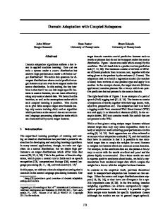
FIG. 1. 共Color online兲 共a兲 Example of an energy- and spindependent lead DOS ␳␴共␻兲 with an additional spin-dependent shift ⌬␴. To perform the logarithmic discretization, a generalized bandwidth D0 is defined. Since we allow for bands with energy and spin dependence, the discretization is performed for each spinˆ does not include component separately, see panel 共b兲. Since H ᐉd spin-flip processes, an impurity electron of spin ␴ 关circles in panel 共b兲兴 couples to lead electrons of spin ␴, ␴ = ↑ 共↓兲, only. Panel 共b兲 also illustrates that impurity electrons couple to leads’ electron and hole states with arbitrary energy ␻, 兩␻兩 艋 D0.

⌬ = ⌬↓ − ⌬↑ ,

共6兲

at the band edges of the conduction band 共see Fig. 10兲. The flat band model with a Stoner splitting and consequences of the particle-hole symmetry breaking is considered in Sec. VI. 3. Arbitrary band structure

1. Flat band

The simplest situation where one can account spin asymmetry is a flat band with the energy-independent DOS ␳␴共␻兲 = ␳␴. Then, the spin asymmetry can be parametrized just by a single parameter, the spin imbalance in the DOS at the Fermi energy ␻ = 0. For flat bands, the knowledge of the spin polarization P of the leads, defined as P=

␳↑共0兲 − ␳↓共0兲 , ␳↑共0兲 + ␳↓共0兲

共5兲

is sufficient to fully parametrize ␳␴共␻兲 共see Fig. 2兲. This particular DOS shape is special due to the fact that the particle-hole symmetry is conserved in the electrodes leading to a particular behavior for the symmetric Anderson model. This type of model of the leads will be considered in Sec. V. 2. Stoner splitting

One can generalize this model and break the particle-hole symmetry by taking the Stoner splitting into account. A consequence of the conduction electron ferromagnetism is that the spin-dependent bands are shifted relative to each other 共see Fig. 1兲. For a finite value of that shift ⌬␴, the spin-␴ band is in the range −D + ⌬␴ 艋 ␻ 艋 D + ⌬␴ 共with the “original” bandwidth D兲. In the limit ⌬␴ = 0, only energies within the interval 关−D ; D兴 are considered, a scheme usually used in the NRG calculations.7 This relative shift between the two spin-dependent bands leads to the so-called Stoner splitting ⌬, defined as

Since the spin splitting of the dot level is determined by the coupling to all occupied and unoccupied 共hole兲 electronic states in the leads, the shape of the whole band plays an important role. Therefore, it is reasonable to consider an arbitrary DOS shape, which cannot be parametrized by a particular set of parameters as the imbalance between ↑ and ↓ electrons at the Fermi energy or a Stoner splitting 共see Fig. 1兲. Therefore, in Sec. VII, we will consider a model with a more complex band structure and, in Sec. III, we will develop the NRG technique for an arbitrary band structure. III. METHOD: NUMERICAL RENORMALIZATION GROUP FOR AN ARBITRARY SPINDEPENDENT DENSITY OF STATES

In our analysis, we take the ferromagnetic nature of the noninteracting leads by means of a spin- and energydependent DOS ␳␴共␻兲 into account. A general example is given in Fig. 1. To compute the properties of the model described above, we have extended the NRG technique calculation to handle a spin-dependent density of states. In order to understand to what extent the method applied here is different from the standard NRG, it is adequate to briefly review the general concepts of NRG. The NRG technique was invented by Wilson in the 1970s to solve the Kondo problem;14 later, it was extended to handle other quantum impurity models as well.24–26,28 In his original work, Wilson considered a spin-independent flat density of states for the conduction electrons. Closely fol-

045321-3

PHYSICAL REVIEW B 76, 045321 共2007兲

SINDEL et al.

lowing Refs. 17 and 27, where the mapping for the case of energy-dependent DOS was given, we generalize that procedure for the case of the Hamiltonian given in Eq. 共4兲 which contains leads with an energy and spin-dependent DOS. It is convenient to bring the Hamiltonian given by Eq. 共4兲 into a continuous representation27 before the generalized mapping is started. The replacement of the discrete fermionic operators by continuous ones, ␣k␴ → ␣␻␴, translates the lead and the tunneling part of the Hamiltonian into ˆ =兺 H ᐉ ␴

ˆ =兺 H ᐉd ␴

冕

冕

1 † d␻g␴共␻兲␣␻␴ ␣␻␴ ,

共7兲

d␻h␴共␻兲共d␴† ␣␻␴ + H.c.兲.

共8兲

−1

lead operators of harmonic index p = 0兲 will be dropped below. Defining a fermionic operator f 0␴ ⬅

ˆ =兺 H ᐉd ␴

As shown in Ref. 27, the hereby defined generalized dispersion g␴共␻兲 and hybridization h␴共␻兲 functions have to satisfy the relation

⳵g␴−1共␻兲 兵h␴关g␴−1共␻兲兴其2 = ␳␴共␻兲关V␴共␻兲兴2 , ⳵␻

共9兲

is the inverse of g␴共␻兲, which ensures that the where action on the impurity site is identical both in the discrete and the continuous representation. Note that there are many possibilities to satisfy Eq. 共9兲. The key idea of Wilson’s NRG14 is a logarithmic discretization of the conduction band, by introducing a discretization parameter ⌳, which defines energy intervals 兴 − D0⌳−n ; −D0⌳−n−1兴 and 关D0⌳−n−1 ; D0⌳−n关 in the conduction band 共n 苸 N0兲. Within the nth interval of width dn = ⌳−n共1 − ⌳−1兲, a ± Fourier expansion of the lead operators ⌿np 共␻兲 with fundamental frequency ⍀n = 2␲ / dn is defined as =

冦

1

冑d n e

±i⍀n p␻

if ⌳−共n+1兲 艋 ± ␻ ⬍ ⌳−n otherwise.

0

冧

␣␻␴ =

再兺 np

冎

+ − 关anp␴⌿np 共␻兲 + bnp␴⌿np 共␻兲兴 .

冋冑

共11兲

共12兲

⬁

ˆ = H ᐉ

† 关␧n␴ f n†␴ f n␴ + tn␴共f n†␴ f n+1␴ + f n+1 兺 ␴ f n␴兲兴. ␴n=0

共13兲

In general, the on-site energies ␧n␴ and hopping matrix elements tn␴ along the Wilson chain need to be determined numerically. Besides the matrix elements ⑀n␴ and tn␴, coefficients unm␴ and vnm␴, which define the fermionic operators f n␴, ⬁

f n␴ ⬅

兺 共unm␴am␴ + vnm␴bm␴兲,

共14兲

m=0

already used in Eq. 共13兲, need to be determined. One immediately anticipates the following from Eq. 共11兲: − 冑 v0m␴ = ␥m ␴/ ␰ 0␴ .

共15兲

Equations which determine the matrix elements ⑀n␴ and tn␴ and the coefficients unm␴ and vnm␴ are given in Appendix B. Note that the on-site energies ␧n␴ vanish in the presence of particle-hole symmetry in the leads. To summarize, Hamiltonians as the one given in Eq. 共4兲 ˆ , can be cast into the form of a linear chain H LC ˆ + 冑␰ /␲ 兺 共d† f + f † d 兲 ˆ =H H LC d 0␴ ␴ 0␴ 0␴ ␴ ␴

⬁

共10兲

Impurity electrons couple only to the p = 0 mode of the lead operators, given that the energy-dependent generalized hybridization h␴共␻兲 is replaced by a constant hybridization, h␴共␻兲 → hn+␴ for ␻ ⬎ 0 共or hn−␴ for ␻ ⬍ 0, respectively兲. Obviously, the particular choice of constant hybridization hn±␴ demands the generalized dispersion g␴共␻兲 to be adjusted accordingly, such that Eq. 共9兲 remains valid. Details of this procedure can be found in Appendix A. Since we adopt this strategy, the harmonic index p 共the impurity couples only to

册

␰ 0␴ † 共d f 0␴ + H.c.兲 . ␲ ␴

+ 冑 u0m␴ = ␥m ␴/ ␰ 0␴,

Here, the subscripts n and p 共苸Z兲 label the corresponding interval and the harmonic index, respectively, while the superscript marks positive 共⫹兲 or negative 共⫺兲 intervals, respectively. The above defined Fourier series now allows one to replace the continuous fermionic conduction band operators a␻␴ by discrete ones anp␴ 共bnp␴兲 of harmonic index p and spin ␴ acting on the nth positive 共negative兲 interval only,

−

The final step in the NRG procedure is the transformation of ˆ into the form of a linear chain. This the conduction band H ᐉ goal is achieved via the tridiagonalization procedure developed by Lánczos,30

g␴−1共␻兲

± 共␻兲 ⌿np

+

1 ⌫␴共␻兲d␻ and the coeffiwith ␰0␴ = 兺n关共␥n+␴兲2 + 共␥n−␴兲2兴 = 兰−1 ± cients ␥n␴ as given in Appendix A,29 reveals that the impurity effectively couples to a single fermionic degree of freedom only, the zeroth site of the Wilson chain 关for further ˆ can details, see Eq. 共A2兲兴. Therefore, the tunneling part of H be written in a compact form as

1

−1

1

共an␴␥n␴ + bn␴␥n␴兲, 冑␰ 0 ␴ 兺 n

+

† 关␧n␴ f n†␴ f n␴ + tn␴共f n†␴ f n+1␴ + f n+1 兺 ␴ f n␴兲兴, ␴n=0

共16兲 even though one is dealing with energy- and spin-dependent leads. In general, however, this involves numerical determination of the matrix elements ␧n␴ and tn␴,17 in contrast to Ref. 24 共where flat bands were considered兲, where no closed analytical expression for those matrix elements is known. Equation 共16兲 nicely illustrates the strength of the NRG procedure. As a consequence of the energy separation guaranteed by the logarithmic discretization, the hopping rate

045321-4

PHYSICAL REVIEW B 76, 045321 共2007兲

KONDO QUANTUM DOT COUPLED TO FERROMAGNETIC…

along the chain decreases as tn ⬃ ⌳−n/2 共the on-site energies decays even faster兲, which allows us to diagonalize the chain Hamiltonian iteratively and, in every iteration, to keep the states with the lowest lying energy eigenvalues as the most relevant ones. This very fact underlines that this method does not rely on any assumptions concerning leading order divergences.31

+ ix / 2␲T兲 and ⌿共x兲 denotes the digamma function. For T = 0, the spin splitting is given by ⌬⑀d ⯝

冉

冊

兩 ⑀ d兩 P⌫ ln , ␲ 兩U + ⑀d兩

共18兲

showing a logarithmic divergence for ⑀d → 0 or U + ⑀d → 0. B. Stoner splitting

IV. PERTURBATIVE SCALING ANALYSIS

We can understand the spin splitting of the spectral function using Haldane’s scaling approach,16 where quantum charge fluctuations are integrated out. The behavior discussed in this paper can be explained as an effect of spindependent quantum charge fluctuations, which lead to a spindependent renormalization of the dot’s level position ˜⑀d␴ and a spin-dependent level broadening ⌫␴, which, in turn, induce spin splitting of the dot level and the Kondo resonance. Within this approach, a spin splitting of the local dot level, ⌬⑀d ⬅ ␦⑀d↑ − ␦⑀d↓ + B, which depends on the full band structure of the leads, is obtained13 where 1 ␦ ⑀ d␴ ⯝ − ␲

冕

再

冎

⌫␴共␻兲关1 − f共␻兲兴 ⌫¯␴共␻兲f共␻兲 d␻ + . ␻ − ⑀ d␴ ⑀d¯␴ + U − ␻

For real systems, particle-hole 共p-h兲 symmetric bands cannot be assumed; however, the compensation ⌬⑀ = 0 using a proper tuning of the gate voltage ⑀d is still possible. We can also analyze the effect of the Stoner splitting by considering a flat band structure in Fig. 2 using the value of the Stoner splitting ⌬ = 0.2共 DD0 兲D0. Then, also from Eq. 共17兲, we can expect an additional spin splitting of the dot level induced by the presence of the Stoner field in the leads even for spin polarization P = 0 given by ⌬⑀共St兲 d ⯝

冋

册

共− ⑀d + D0 − ⌬兲共U + ⑀d + D0 − ⌬兲 ⌫ ln , 2␲ 共− ⑀d + D0兲共U + ⑀d + D0兲 共19兲

which, for the symmetric level position, ⑀d = −U / 2, leads to

共17兲

Note that the splitting is not only determined by the lead spin polarization P, i.e., the splitting is not only a property of the Fermi surface. Equation 共17兲 is the key equation to explain the physics of the 共spin-dependent兲 splitting of the local level ⑀d␴. This equation explains the spin-dependent occupation and, consequently, the splitting of the spectral function of a dot that is contacted to leads with a particular band structure. The first term in the curly brackets corresponds to electronlike processes, namely, charge fluctuations between a single occupied state 兩␴典 and the empty 兩0典 one, and the second term to holelike processes, namely, charge fluctuations between the states 兩␴典 and 兩2典. The amplitude of the charge fluctuations is proportional to ⌫, which, for ⌫ Ⰷ T, determines the width of dot levels observed in transport. The exchange field given by Eq. 共17兲 giving rise to precession of an accumulated spin on the quantum dot attached to leads with noncollinear leads’ magnetization is not discussed here.23

⌬⑀共St兲 d ⯝

冉

冊

U/2 + ⑀d + D0 − ⌬ ⌫ ln , ␲ U/2 + ⑀d + D0

共20兲

Equation 共19兲 also shows that the characteristic energy scale of the spin splitting is given by ⌫ rather than by the Stoner splitting ⌬ 共⌬ Ⰷ ⌫兲, since the states far from the Fermi surface enter Eq. 共17兲 only with a logarithmic weight. The difference can be as large as 3 orders of magnitude, so, in a metallic ferromagnet, the Stoner splitting energy is of the genorder ⌬ ⬃ 1 eV but the effective molecular field ⌬⑀共St兲 d

A. Flat band

Equation 共17兲 predicts that even for systems with spin asymmetric bands ␳↑共␻兲 ⫽ ␳↓共␻兲, the integral can give ⌬⑀ = 0, which corresponds to a situation where the renormalization of ⑀d␴ due to electronlike processes is compensated by holelike processes. An example is a system consisting of particle-hole symmetric bands, ␳␴共␻兲 = ␳␴共−␻兲, where no splitting of the Kondo resonance 共⌬⑀d = 0兲 for the symmetric point, ⑀d = −U / 2, appears. For a flat band, ␳␴共␻兲 = ␳␴, Eq. 共17兲 can be integrated analytically. For D0 Ⰷ U, 兩⑀d兩, one finds where ␾共x兲 ⬅ ⌿共 21 ⌬⑀ ⯝ 共P⌫ / ␲兲Re关␾共⑀d兲 − ␾共U + ⑀d兲兴,

FIG. 2. 共Color online兲 The lead density of states of a flat 关␳s共␻兲 = ␳␴兴 but spin-dependent 共␳↑ ⫽ ␳↓兲 band for spin polarization P = 0.2. The dark region marks the filled states below the Fermi energy. Since ⌬↑ = ⌬↓ = 0, the generalized bandwidth D0 = D.

045321-5

PHYSICAL REVIEW B 76, 045321 共2007兲

SINDEL et al.

erated by it is still a small fraction of ⌫—of order of 1 meV, comparable with the Kondo energy scale for molecular single-electron transistors.10 However, the Stoner splitting introduces a strong p-h asymmetry, so it can influence the character of the gate voltage dependence significantly. In the next section, we analyze the effect of different types of the band structure using numerical renormalization group technique and compare it to that obtained in this section by scaling procedure.

0.75

a

0.25

1

εd=−U/3

n↑

n↓

b

A. Spin and charge state

Consequently, we start our numerical analysis by comput¯ ␴典, which is a ing the spin-resolved dot occupation n␴ ⬅ 具n static property. Figure 3 shows the spin resolved impurity occupation as a function of the spin polarization P of the leads. Figure 3共a兲 and 3共c兲 correspond to a gate voltage of ⑀d = −U / 3 共where the total occupation of the system n↑ + n↓ ⬍ 1兲 whereas the second line corresponds to ⑀d = −2U / 3 共with n↑ + n↓ ⬎ 1兲. The total occupation of the system, n↑ + n↓, decreases 共increases兲 for ⑀d = −U / 3 共⑀d = −2U / 3兲 when the spin polarization of the leads is finite, P ⫽ 0. Note that both situations, ⑀d = −U / 3 and ⑀d = −2U / 3, are symmetric with respect to changing particle into hole states and vice versa, which is possible only for the leads with particle-hole symmetry. For the gate voltage ⑀d = −U / 2, there is a particlehole symmetry in the whole system leads with a DOS which does share this symmetry even in the presence of spin asymmetry. Note that whereas a finite spin polarization leads to a decrease in n↑ + n↓ for ⑀d ⬎ −U / 2 关see Fig. 3共a兲兴, it results in an increase in n↑ + n↓ for ⑀d ⬍ −U / 2 关see Fig. 3共b兲兴. Obviously, for P = 0 and in the absence of an external magnetic field, the impurity does not have a preferred occupation, n↑ = n↓. Any finite value of P violates this relation: n↑ ⬎ n↓ for P ⬎ 0 and ⑀d ⬎ −U / 2 共since ␦⑀d↑ ⬃ ⌫↓ ⬍ ⌫↑ ⬃ ␦⑀d↓兲. For ⑀d ⬍ −U / 2, on the other hand, the opposite behavior is found.

n↑

n↓

n↓

n↑ −0.5

0.5

P

d

n↓

n↑+n↓

εd=−2U/3

0.5

V. FLAT BANDS WITHOUT STONER SPLITTING

c

n↑+n↓

n↑+n↓

n↑+n↓

We start our analysis by considering normalized flat bands without the Stoner splitting 共i.e., D0 = D兲, as sketched in Fig. 2, with finite spin polarization P ⫽ 0 关defined via Eq. 共5兲兴.32 In this particular case of spin 共but not energy兲 dependent coupling, ⌫␴ ⬅ ␲␳␴V2, the coupling ⌫␴ can be parametrized via P, ⌫↑共↓兲 = 21 ⌫共1 ± P兲 关here, ⫹ 共⫺兲 corresponds to spin ↑ 共↓兲兴, where ⌫ = ⌫↑ + ⌫↓. Leads with a DOS as the one analyzed in this section have, for instance been studied in Refs. 7 and 8. Since ⌫␴ ⬅ ␲␳␴V2, the spin dependence of ⌫␴ can be ab1 sorbed by replacing V → V␴ = V冑 2 共1 ± P兲 in Eq. 共4兲, i.e., a spin-dependent hopping matrix element, while treating the leads as unpolarized ones 共␳␴ → ␳兲. This procedure has the particular advantage that the “standard” NRG procedure24 can be applied, meaning that the on-site energies 共tunneling matrix elements兲 关defined in Eq. 共13兲兴 along the Wilson chain ␧n␴ vanish, while tn␴ turn out to be spin independent. Therefore, it does not involve the solution of the tedious equations given in Appendix B.

B / Γ=−0.1

B=0

n↑ −0.5

0.5

P

FIG. 3. 共Color online兲 关共a兲–共d兲兴 Spin-dependent occupation n␴ of the local level as a function of the leads’ spin polarization P for ⑀d = −U / 3 关共a兲 and 共c兲兴 and ⑀d = −2U / 3 关共b兲 and 共d兲兴 共related by the particle-hole symmetry兲 for B = 0 共left column兲 and B = −0.1⌫ 共right column兲. For finite spin-polarization, P ⫽ 0, the condition n↑ = n↓ can only be obtained by an appropriately tuned magnetic field, as shown in 共c兲 and 共d兲. Parameters: U = 0.12D0 and ⌫ = U / 6.

The effect on the impurity of a finite lead polarization, namely, to prefer a certain spin species, can be compensated by a locally applied magnetic field, as shown in Figs. 3共c兲 and 3共d兲. For ⑀ = −U / 3 and B / ⌫ = −0.1 关see Fig. 3共c兲兴, the impurity is not occupied by a preferred spin species, n↑ = n↓, for P ⬃ 0.5. Due to particle-hole symmetry, the same magnetic field absorbs a lead polarization of P ⬃ −0.5 for ⑀ = −2U / 3 关see Fig. 3共d兲兴. The magnetic field which restores the condition n↑ = n↓, henceforth denoted as compensation field Bcomp共P兲, will be of particular interest below. B. Single-particle spectral function

Using the NRG technique we can access the spin-resolved single-particle spectral density A␴共␻ , T , B , P兲 = R 共 ␻ 兲 for arbitrary temperature T, magnetic field B, − ␲1 Im Gd, ␴ and spin polarization P, where G␴R共␻兲 denotes a retarded Green function. We can relate the asymmetry in the occupancy, n↑ ⫽ n↓, to the occurrence of charge fluctuations in the dot and broadening and shifts of the position of the energy levels 共for both spins up and down兲. For P ⫽ 0, the charge fluctuations, and hence level shifts and level occupations, become spin dependent, causing the dot level to split6 and the dot magnetization n↑ − n↓ to be finite. As a result, the Kondo resonance is also spin split and suppressed 关Fig. 4共b兲兴, similarly to the effect of an applied magnetic field.33 This means that Kondo correlations are reduced or even completely suppressed in the presence of ferromagnetic leads. Note the asymmetry in the spectral function for P ⫽ 0 which stems from the spin-dependent hybridization ⌫␴. Figure 4共b兲, where the spin-resolved spectral function is plotted, reveals the origin of the asymmetry around the Fermi energy of the spectral function. The spectral function obtained for polarized leads has to be contrasted to that of a dot asserted

045321-6

PHYSICAL REVIEW B 76, 045321 共2007兲

KONDO QUANTUM DOT COUPLED TO FERROMAGNETIC…

εd=−U/3 εd=−U/2 εd=−7U/12

1

0 −0.05

0

Bcomp / Γ

P=0.0 P=0.2 P=0.4 P=0.6

0.2

0.05

1

a

0

P=0.0 P=0.4 P=0.8

0.6 0.4 0.2

−0.2

−1

0

0 −0.05

1

0

0

ω/U

0.05

0 −0.05

FIG. 5. 共Color online兲 共a兲 Compensation field Bcomp共P兲 for different values of ⑀d. For flat bands, Bcomp depends linearly on the lead polarization. At the point where there is particle-hole symmetry, so for gate voltage 共⑀d = −U / 2兲, Bcomp共P兲 = 0 for any value of P, i.e., the spectral function is not split for any value of P even though B = 0. 共b兲 Spectral function for various values of P for B = Bcomp. Note the sharper resonance in the spectral function, i.e., a reduced Kondo temperature TK.

εd=−2U/3

c

0

ω/U

0.05

FIG. 4. 共Color online兲 Total spectral functions A共␻兲 = 兺␴A␴共␻兲 for various values of the spin polarization P. 共a兲 For ⑀d = −U / 3, an increase in P results in a splitting and suppression of the Kondo resonance 共see inset兲. The effect of finite P on the Hubbard peaks is less significant. The spin-resolved spectral function A␴共␻兲, shown in 共b兲, reveals that A↑共␻兲 and A↓共␻兲 differ significantly from each other for P ⫽ 0. 共c兲 Spectral function for the same values of P as in 共a兲 but for ⑀d = −2 / 3U 关due to particle-hole symmetry, the results are mirrored as compared to 共a兲 but with inverted spins兴. Parameters: U = 0.12D0, B = 0, and ⌫ = U / 6.

to a local magnetic field, where a nearly symmetric 共perfect symmetry is only for the symmetric Anderson model兲 suppression and splitting of the Kondo resonance 共around the Fermi energy兲 appear.33 In Fig. 4共c兲, the gate voltage 共⑀d = −2U / 3兲 is chosen such that it is particle-hole symmetric to the case shown in Fig. 4共a兲. Due to the opposite particle-hole symmetry, the obtained spectral function in Fig. 4共c兲 is nothing else but the spectral function shown in Fig. 4共a兲 mirrored around the Fermi energy. Figures 3共c兲 and 3共d兲 showed that a finite magnetic field B can be used to recover the condition n↑ = n↓. Indeed, for any lead polarization P, a compensation field Bcomp共P兲 exists at which the impurity is not preferably occupied by a particular spin species. To a good approximation, Bcomp共P兲 has to be chosen such that the induced spin splitting of the local level is compensated.36,37 One consequently expects a linear P dependence of Bcomp from Eq. 共18兲. Figure 5共a兲 shows the P dependence of Bcomp for various values of ⑀d obtained via NRG. The numerically found behavior can be explained through Eq. 共18兲. It confirms that the slope of Bcomp is negative 共positive兲 for ⑀d ⬎ −U / 2 共⑀d ⬍ −U / 2兲 and that Bcomp共P兲 = 0 for ⑀d = −U / 2. The fact that this occurs simultaneously with the disappearance of the Kondo resonance splitting suggests that the local spin is fully screened at Bcomp. The expectation of an unsplit Kondo resonance in the presence of the magnetic field Bcomp is nicely confirmed by our numerics in Fig. 5共b兲 for ⑀d = −U / 3. Moreover, the sharpening of the Kondo resonance in the spectral function upon increasing P 共indicating a decrease in the Kondo temperature TK兲 can be extracted from this plot. The associated binding energy of the singlet 共the

Kondo temperature TK兲 is consequently reduced. Having demonstrated that the Kondo resonance can be fully recovered for Bcomp even though P ⫽ 0, we show that there is also the possibility to recover the unsplit Kondo resonance via an appropriately tuned gate voltage. In Fig. 6, we plot the spin-resolved spectral function for various values of ⑀d for P = 0.2 and B = 0. Note that one can easily identify whether the Kondo resonance is fully recovered from the positions of A␴共␻兲 relative to each other. Since a dip in the total spectral function A共␻兲 = 兺␴A␴共␻兲 is not present for a modest shift of A␴共␻兲 with respect to each other, we identify an unsplit Kondo resonance with perfectly aligned spinresolved spectral functions henceforth. Clearly, one can identify from Fig. 6 that the spectral function is split for any value ⑀d ⫽ −U / 2. This splitting changes its sign at ⑀d = −U / 2. For the particular case ⑀d = −U / 2 关see Fig. 6共b兲兴, the spectral function reaches the uni1

πΓAσ(ω)/4

0 −0.05

b

1

πΓA(ω)/4

πΓAσ(ω)/2

εd=−U/3 P=0.4

1

ω/U

a

b

εd=−U/3

εd=−U/2

σ=↑+↓ σ=↑ σ=↓

0.5

1

πΓAσ(ω)/4

−1

1

0.05

ω/U

P

0

b

εd=−U/3

0.8

πΓA(ω)/4

εd=−U/3 πΓA(ω)/4

a

πΓA(ω)/4

1

P=0.2

c

εd=−7U/12

εd=−5U/6

d

0.5

−0.05

0

ω/U

0.05

−0.05

0

0.05

ω/U

FIG. 6. 共Color online兲 Spin-dependent spectral function A␴共␻兲 for various values of ⑀d, fixed P = 0.2, and B = 0 关共blue兲 dashed: A↑共␻兲; 共green兲 long dashed: A↑共␻兲; 共red兲 dotted: A共␻兲 = 兺␴A␴共␻兲兴. The splitting between A↑ and A↓ changes its sign at ⑀d = −U / 2. The spectral function A共␻兲 is plotted for several values of P for ⑀d = −U / 3 in Fig. 4共a兲. The splitting of the spectral function A共␻兲 depends on P as well on ⑀d. Parameters: U = 0.12D0 and ⌫ = U / 6.

045321-7

PHYSICAL REVIEW B 76, 045321 共2007兲

SINDEL et al.

Im χS (ω)/[π/ TK(P)]

10

sin2共␲n␴兲 , ␲⌫␴

共21兲

where ␾␴ is the spin-dependent phase shift. This implies a split and suppressed Kondo resonance for P ⫽ 0 in the absence of a magnetic field. An equal spin occupation, n↑ = n↓, can be obtained only for an appropriate external magnetic field B = Bcomp. For the latter, in the local moment regime 共n ⬇ 1兲, we have n↑ = n↓ ⬇ 0.5, so that ␾↑ = ␾↓ ⬇ ␲ / 2, which implies that the peaks of A↑ and A↓ are aligned. Thus, the Friedel sum rule clarifies why the magnetic field Bcomp at which the splitting of the Kondo resonance disappears coincides with that for which n↑ = n↓. Equation 共21兲 indicates a new feature, namely, that the amplitude of the Kondo resonance becomes spin dependent 共see also the discussion in Sec. V E兲. It is important to point out that Eq. 共21兲 is valid only for the leads with particle-hole symmetry 共see Ref. 35兲. For an arbitrary DOS shape, it is possible to generalize the Friedel sum rule.

−4

P=0.0 P=0.2 P=0.4 P=0.6 P=0.8

10

共22兲

共F denotes the Fourier transform兲 关see also Fig. 7共a兲兴, in the presence of the appropriate Bcomp共P , ⑀d兲 and identified the maximum in Im ␹zS with TK共P兲. Figure 8共a兲 shows TK共P兲 normalized to TK共P = 0兲 for different values of ⑀d. As shown in Refs. 6 and 7, the functional dependence of TK共P兲 can be

10

−4

−2

10

0

10 ω/TK(P)

10

2

b

0

4

10

B=Bcomp(P) εd=−U/3 −4

−2

0 2 ω/T K(P)

4

FIG. 7. 共Color online兲 The isotropic Kondo effect, accompanied by universal scaling, can be recovered even for P ⫽ 0 and B = Bcomp since both 共a兲 the spin-susceptibility Im ␹zS and 共b兲 the spectral function collapse onto a universal curve. This statement holds for any value of ⑀d with some corresponding compensation fields, as given in Fig. 5共a兲. Parameters: U = 0.12D0, ⑀d = −U / 3, and ⌫ = U / 6.

nicely explained within the framework of a poor man’s scaling. Note that the decrease in TK is rather weak for a modest value of P. In Fig. 7共b兲, we plot, in addition to TK共P兲, the gate voltage dependence of TK共⑀d兲 normalized to TK共⑀d = −U / 2兲 共where the Kondo temperature is minimal兲 for fixed P = 0.2. In the presence of Bcomp共P , ⑀d兲, this functional dependence of the Kondo temperature can be analytically described via Haldane’s formula16 for the Kondo temperature of a single-level dot coupled to unpolarized leads, TK = 21 冑U⌫e␲⑀d共⑀d+U兲/⌫U. This fact is another manifestation that indeed the usual Kondo effect can be recovered in the presence of spin-polarized leads, given that the appropriate Bcomp共P , ⑀d兲 is applied. Having shown that the coexistence of spin polarization in the leads and the Kondo effect is possible 共given that a magnetic field B is tuned appropriately at a given gate voltage ⑀d兲, we plot the properly rescaled spin susceptibility Im ␹zS 关see Fig. 7共a兲兴, and the spectral function 关see Fig. 7共b兲兴, confirming that the isotropic Kondo effect is recovered. The expected collapse of Im ␹zS and 兺␴⌫␴A␴共␻兲 onto a universal 1

10

a analytic

0.8 0.6

εd=−U/3 εd=−U/2 εd=−7U/12

0.4 0.2 0

We already stated above that the Kondo temperature TK decreases when the lead polarization P is increased. Obviously, TK has to vanish when we are dealing with fully spinpolarized leads, 兩P 兩 = 1. To obtain TK共P兲, we calculated the imaginary part of the quantum dot spin spectral function,

−6

10 10

D. Spin-spectral function: Kondo temperature

␹zS共␻兲 = F兵i⌰共t兲具关Sz共t兲,Sz共0兲兴典其

10

TK(ε)/TK(ε=−U/2)

A␴共0兲 =

1

B=Bcomp(P) εd=−U/3

−8

TK(P)/TK(0)

A direct consequence of the spin splitting of the local level and the accompaning n↑ ⫽ n↓ for P ⫽ 0 and B = 0 can be explained by means of the Friedel sum rule,34 an exact T = 0 relation valid also for arbitrary values of P and B. This formula relates the height of the spectral function 共at the Fermi energy兲 and the phase shift of the electrons scattered by the impurity. As already pointed out, spin-polarized electrodes induce a splitting, the local impurity level resulting in a spin-dependent occupation of the impurity. Thus, the knowledge of the local occupation can be used to anticipate 共via the Friedel sum rule兲 that the local spectral function becomes spin split and suppressed 共similar to the presence of a local magnetic field兲 in the presence of spin-polarized leads. According to the Friedel sum rule, the height of the spectral function at the Fermi energy A␴共0兲 is fully determined by the level occupation n␴,

␾ ␴ = ␲ n ␴,

a

−2

z

C. Friedel sum rule

0

π Σσ Aσ(ω)Γσ/2

tary limit. For this gate voltage, the spin-resolved spectral functions A␴共␻兲 have a different height, as predicted from the Friedel sum rule 关Eq. 共21兲兴.

0

0.2

0.4

P

0.6

0.8

8

b

P=0.2

6

analytic

4 2 0 −0.5

−0.4

−0.3

ε/U

−0.2

−0.1

FIG. 8. 共Color online兲 共a兲 Spin polarization dependence of the Kondo temperature TK共P兲 关obtained by applying an appropriate B = Bcomp共P , ⑀d兲兴. The functional dependence of TK共P兲 found via a poor man’s scaling analysis 共dotted line兲 关see Eq. 共6兲 of Ref. 6兴 is confirmed by the NRG analysis. The plot confirms that a dot tuned to the local moment regime, 兺␴n␴ ⯝ 1, shows the universal P dependence of TK共P兲 for arbitrary values of ⑀d. 共b兲 The ⑀d dependence of TK for fixed P = 0.2 at B = Bcomp. As long as the impurity remains in the local moment regime, Haldane’s formula 共Ref. 16兲 for TK 共dotted line兲 properly describes TK共⑀d兲 even though the leads have a finite spin polarization. Parameters: U = 0.12D0 and ⌫ = U / 6.

045321-8

PHYSICAL REVIEW B 76, 045321 共2007兲

KONDO QUANTUM DOT COUPLED TO FERROMAGNETIC… 1.1

Gσ [e /h]

b

2

1

0.9

a

πΓAσ(ω=0)/2

10

up down 1/(1±P)

8 6 4 2 0

−1

−0.5

0

0.5

1

P FIG. 9. 共Color online兲 共a兲 Height of the spin-resolved spectral function A␴共␻ = 0兲 as a function of P. The dashed line shows the 1 / 共1 ± P兲 dependence as expected from the Friedel sum rule 关Eq. 共21兲兴. 共b兲 Spin-resolved conductance G␴ as obtained from Eq. 共23兲. This plot confirms the expectation based on the Friedel sum rule that the spin-resolved conductance should be independent of the spin species, consequently, it serves as a consistency check of our numerics.

FIG. 10. 共Color online兲 The DOS in the case of flat bands with the Stoner splitting ⌬ and a finite spin polarization P. In general, the shifts of the ↑ and ↓ bands are unrelated to each other, ⌬↓ ⫽ −⌬↑. In this section, however, we assume ⌬↓ = −⌬↑. VI. FLAT BANDS WITH STONER SPLITTING

curve for temperatures below TK 关note that TK depends on P, see, e.g., Fig. 5共b兲兴 is confirmed by our numerical results. For energies much bigger than TK, ␻ Ⰷ TK, universal scaling is lost and the curves start to deviate from each other. E. Conductance

The knowledge of the spectral function enables us to compute quantities which are experimentally accessible, such as the linear conductance. To investigate the question whether spin-polarized ferromagnetic leads introduce a spindependent current, we compute the spin-resolved conductance G␴, G␴ =

e2 2⌫L␴⌫R␴ ប 共⌫L␴ + ⌫R␴兲

冕

⬁

−⬁

冋

d ␻ A ␴共 ␻ 兲 −

册

⳵ f共␻兲 , ⳵␻

共23兲

with f共␻兲 denoting the Fermi function 共remember that we choose ⌫L␴ = ⌫R␴兲. The total conductance G is nothing else but the sum of the spin-resolved conductances G = 兺␴G␴. Based on the Friedel sum rule 关Eq. 共21兲兴, we expect the height of the spin-resolved spectral function at the Fermi energy A␴共0兲 ⬃ 1 / ⌫␴ ⬃ 1 / 共1 ± P兲. This expectation is nicely confirmed by our numerical results in Fig. 9共a兲. As the T = 0 conductance is given by the product of A␴共0兲 and ⌫␴, the spin-resolved conductance G␴ ⬃ ⌫␴A␴共0兲 becomes P independent. The results of the NRG calculation are shown in Fig. 9共b兲, confirming this expectation. We conclude that, even though one is dealing with spin-polarized leads, it is not possible to create a spin current via spin-polarized leads; the current remains spin independent. For the antiparallel alignment due to the DOS mismatch, the conductance will be reduced below the G0 = 2e2 / h limit.

In ferromagnetic leads, in addition to a finite lead spin polarization P at the Fermi surface, a splitting between the spin-↑ and spin-↓ bands, ⌬␴ 共Stoner splitting兲, which is an effect of the effective exchange magnetic field in the leads, might appear. Taking this effect into account we do not expect the splitting of the Kondo resonance to disappear at ⑀d = −U / 2, as in Fig. 6共b兲, rather at a different value of ⑀d determined by the shifts ⌬␴. This is due to the fact that the Stoner splitting breaks the particle-hole symmetry in the electrodes. Consequently, we shall consider flat, spinpolarized leads 共of polarization P兲, which are shifted relative to each other by an amount ⌬␴ in this section. Since particlehole symmetry is lost for this band structure, in the leads, we expect neither the splitting of the Kondo resonance, see, e.g., Fig. 6, nor the compensation field Bcomp to be symmetric around ⑀d = −U / 2, in contrast to Sec. V. To quantify the statement that a shift ⌬␴ introduces a finite exchange field and splitting, in this section we analyze the particular case ⌬↓ = −⌬↑ = ⌬, sketched in Fig. . Note that the lead DOS structure discussed in this section38 already requires the use of the extended NRG scheme, explained in Sec III. In particular, spin-dependent on-site energies along the Wilson chain ⑀n␴, as explained in Sec. III and Appendixes A and B, need to be determined to solve for the lead band structure shown in Fig. 10. The studies summarized in Sec. V revealed that the spinresolved impurity occupation n␴ is the key quantity in the context of a dot contacted to spin-polarized leads. Following this finding, we plot n␴ vs P for leads with ⌬ = 0.1共 DD0 兲D0 and ⑀d = −U / 3 in Fig. 11. In contrast to the previous section, the impurity is preferably occupied by ↓ electrons in the absence of a magnetic field 关see Fig. 11共a兲兴 even for P = 0. A finite magnetic field, e.g., B / ⌫ = 0.1 关Fig. 11共b兲兴, has the same con-

045321-9

PHYSICAL REVIEW B 76, 045321 共2007兲

SINDEL et al. 0.5

0.25

n↑

n↓

0.75

0.25

0

0 −10

b

−0.2

−1

−0.5

0

0.5

1

P

n↑+n↓

B/Γ=0.1

n↑

n↓

−0.5

145 mK

0 ω/TK

TK=500mK

εd=−U/3 εd=−U/2 εd=−7U/12

Vg=−5.10 V

U=53.7 meV

Γ=12.4 meV

0.5

P

FIG. 11. 共Color online兲 Spin polarization P dependence of the local occupation n␴ for 共a兲 B = 0 and 共b兲 B = 0.1⌫ with ⑀d = −U / 3. The Stoner splitting ⌬ even in the absence of spin polarization of the leads, P = 0, introduces an effective exchange field which splits the local level n↓ ⬎ n↑ in the absence of an external magnetic field B = 0. The spin polarization dependence of Bcomp for various values of ⑀d is shown in 共c兲. To a good approximation, the Stoner splitting introduces a constant exchange field 共here, Bcomp / ⌫ ⬇ 0.061兲; therefore, it does nothing else but shift the Bcomp dependence of Sec. V. D D Parameters: U = 0.12共 D0 兲D0, ⌫ = U / 6, and ⌬↓ = −⌬↑ = 0.10共 D0 兲D0.

sequence as described before, namely, the shift of the local impurity levels ⑀d␴. The P dependence of Bcomp for the particular band structure sketched in Fig. 10 is shown in Fig. 11共c兲; it is roughly given by the compensation field for flat bands 关Fig. 5共a兲兴, where the same gate voltages were used, shifted by an effective exchange field ⌬⑀共St兲 d generated by the band splittings for P = 0. The value of BStoner can be obtained via integrating out those band states of energy ␻ which lie in the interval D 艋 兩␻兩 艋 D0 关see Eq. 共20兲兴. The value of this effective exchange field, which is logarithmically suppressed 共as can be shown by perturbative scaling兲 is given by Eq. 共20兲. Inserting the numbers used in this section, we obtain a ⌬⑀共St兲 The numerical calculation reveals d / ⌫ ⬇ 0.060. 共St兲 ⌬⑀d / ⌫ ⬇ 0.061 关see Fig. 11共c兲兴, i.e., the numerical result agrees reasonably well with the result based on the scaling analysis 共see Sec. IV兲. Finite temperature: Comparison with experimental data

In a recent experiment of Nygård et al.11 an anomalous splitting of the zero bias anomaly in the conductance induced by the Kondo resonance in the absence of a magnetic field was observed. In this experiment, quantum dot based on single wall carbon nanotubes contacted to nonmagnetic, spin unpolarized Cr/ Au electrodes were used. Those authors related the observed splitting of the Kondo resonance at zero magnetic field with the presence of a ferric iron nitrate nanoparticle,39 which, due to electronic tunnel coupling to the dot, introduces a spin-dependent hybridization. We model the setup of Ref. 11 by means of a single-level dot tuned to the local moment regime ⑀d␴ = −U / 2 关dashed line in Fig. 1共b兲 of Ref. 11兴. Moreover, we used TK = 500 mK,40 which is roughly the value of TK observed in

0 −10

10

0.5

0 ω/TK

0 −10

10

0.5

220 mK

0 ω/TK

10

550 mK

πΓA(ω)/4

B=0

πΓA(ω)/4

Bcomp / Γ

n↑+n↓

0.2

0.5

80 mK

πΓA(ω)/4

a

0.75

0.5

0K

πΓA(ω)/4

c

πΓA(ω)/4

εd=−U/3

∆=134.3 meV P=0.1

0 −10

0 ω/TK

10

0 −10

0 ω/TK

10

FIG. 12. 共Color online兲 Spin-resolved equilibrium spectral function A␴共␻ , T , V = 0兲 with parameters extracted from Ref. 11. The 共blue兲 dashed lines correspond to A↑共␻ , T , V = 0兲, the 共green兲 long dashed lines to A↓共␻ , T , V = 0兲, and the 共red兲 solid ones to the sum of both, i.e., A共␻ , T , V = 0兲. 关共a兲–共e兲兴 A gradual increase in the temperature for those temperatures used in Ref. 11. For comparison, we plot the T = 0 spectral function A共␻ , T = 0 , V = 0兲 in panel 共a兲 as well. Note that the splitting of the Kondo resonance disappears upon increasing T.

Ref. 11, as an input parameter and extracted U / ⌫ = 4.3 from this value. Since a splitting of the Kondo resonance was observed for ⑀d␴ = −U / 2, see, e.g., Fig. 1共b兲 of Ref. 11, a particle-hole asymmetry must exist to achieve a splitting. We try to model this effect by a using flat band structure and by introducing the Stoner splitting. We find the best agreement between the experimentally observed splitting of the Kondo resonance for ⌬ / U = 2.5. The presence of the nanoparticle introduces a spin-dependent hybridization which we parametrize via the lead spin polarization P. The comparison of the dI / dV vs V characteristics of Ref. 11 with the theoretical result turns out to be rather complicated as it involves the nonequilibrium spectral function A共␻ , T , V兲 which itself is not known how to compute accurately.41,42 It is possible to compare qualitatively the splitting in the nonequilibrium conductance obtained in the experiment to the single-particle spectral function. Due to the splitting in the particle spectral function for the dot, which is strongly related to the low-bias conductance measurements, we find close similarity between both of them. When we approximate the experimental results of dI / dV with A共␻ , T , V = 0兲, we achieve the best agreement between theory and experiment for P = 0.1. For these parameters 共⑀d␴ = −U / 2, U / ⌫ = 4.3, ⌬ / U = 2.5, and P = 0.1兲, we compute the temperature-dependent equilibrium spectral function A共␻ , T , V = 0兲 presented in Fig. 12. The numerical findings shown in Fig. 12 qualitatively confirm the behavior found in the experiment of Nygård et al., namely, vanishing splitting in the dI / dV curves with increasing temperature. In the experiment, however, the differential conductance dI / dV turns out to be asymmetric around

045321-10

PHYSICAL REVIEW B 76, 045321 共2007兲

KONDO QUANTUM DOT COUPLED TO FERROMAGNETIC…

0.2

0

0.4

(a) πΓA(ω=0)/4

πΓΑ(ω=0)/4

0.4

100

1000 T [mK]

(b)

0.2

0

100

1000 T [mK]

FIG. 13. 共Color online兲 Linear conductance as a function of temperature 共a兲 for the model studied in this section and 共b兲 for the case of a dot coupled to normal spin unpolarized leads 共P = 0 and ⌬ = 0兲 but in the presence of a magnetic field B = 0.02U. In both cases, a plateau in the linear conductance around TK can be observed. Whereas the spin-resolved linear conductance is degenerate in case 共b兲 共since it is the symmetric Anderson model with particlehole symmetry兲, this is not the case for 共a兲. Parameters are as in Fig. 12 except for P = ⌬ = 0 in case 共b兲.

the Fermi energy 关see Figs. 2共b兲–2共d兲 in Ref. 11兴. We attribute the asymmetry in the dI / dV curve to the asymmetry in the coupling between left and right leads. Finally, we want to compare the temperature dependence of the linear conductance G found in Ref. 11 关see Fig. 2共a兲 of Ref. 11兴 with the one based on the model described above. In the absence of a magnetic field B = 0 and source-drain voltage V = 0, a plateau in G was found around T ⬇ 500 mK in the experiment. Note that the calculation of G does not involve the nonequilibrium spectral function so we can calculate it exactly. In Fig. 13共a兲, we show the theoretical curve of the spin-resolved conductance G␴ obtained via Eq. 共23兲 for the model discussed in this section. In agreement with the experiment, a plateau in the linear conductance G is found around TK. For comparison, we also plot the linear conductance of a dot contacted to normal spin-unpolarized leads 共i.e., flatbands with P = 0 which are not shifted relative to each other兲 for increasing temperature but in the presence of a finite magnetic field B = 0.02U in Fig. 13共b兲. Such a magnetic field might, e.g., be inserted in to the system via the presence of the ferromagnetic nanoparticles. Also, such a scenario leads to a plateau in G. The value of the associated magnetic field, however, is rather big, B = 0.02U, corresponding to B ⬇ 1 T 关here, we assumed g = 2.0 for the conduction electrons in the nanotube 共see also Ref. 11兲兴. According to Ref. 11, the latter scenario can therefore not explain the observed behavior, since one can argue that such a large magnetic field can hardly be believed to exist in this experiment 共see, in particular, footnote 13 of Ref. 11兲. Consequently, the presence of ferromagnetic leads might explain the experimental observation. We can, however, not exclude other possible mechanisms—such as the existence of an effective magnetic field—which might lead to the observed behavior but, only from special geometry, where the strong stray magnetic field is possible. VII. BAND STRUCTURE WITH ARBITRARY SHAPE

Flat bands, studied in the previous sections, are only a poor approximation of a realistic band structure in the

leads.43 We complete our study by analyzing the effect of an arbitrary lead DOS. Consequently we are considering leads with a DOS which is energy and spin dependent and additionally contains a Stoner splitting in this section. As outlined in the previous section, the “generalized” NRG formalism introduced in Sec. III has to be used in this case as well. In particular, we study the effect of gate voltage variation on the spin splitting of the local level of a quantum dot attached to ferromagnetic leads. We show how the gate voltage can control the magnetic properties of the dot. A similar proposal, namely, to control the magnetic interactions via an electric field, was recently made in gated structures.44 In an analysis of several types of band structures, we found three typical gate voltage dependences of the Kondo resonance. To be more specific, to illustrate this behavior, we used a square-root shape DOS or parabolic band 共as for free s-type electrons兲45 with the Stoner splitting ⌬ 共Ref. 46兲 and some additional spin asymmetry Q,

␳ ␴共 ␻ 兲 =

1 3冑2 −3/2 D 共1 + ␴Q兲冑␻ + D + ␴⌬/2, 2 8

共24兲

depicted in Fig. 14 关␴ ⬅ 1共−1兲 for ↑共↓兲兴. This example turns out to encompass three typical classes mentioned above. Note that we restricted the DOS in Eq. 共24兲 ␻ 苸 关−D − ␴⌬ / 2 , D − ␴⌬ / 2兴 to ensure that we are dealing with a normalized DOS. The three typical gate voltage dependences of the Kondo resonance we found are 共i兲 a scenario where the splitting of the local level was roughly independent of gate voltage 关Fig. 15共a兲兴, 共ii兲 a scenario with a strong gate voltage dependence of the splitting but without compensation 关Fig. 15共b兲兴, and 共iii兲 a case with a strong gate voltage dependence of the splitting including a particular gate voltage where the splitting vanishes 关Fig. 15共c兲兴. Figures 16共a兲–16共c兲 show the effect of an external magnetic field for Figs. 15共a兲–15共c兲, respectively. As already outlined in the previous sections, an external magnetic field can be used to compensate the lead induced spin splitting 共which itself depends on gate voltage兲 and thereby change that gate voltage where the full Kondo resonance exists 关see Figs. 15共c兲 and 16共c兲兴. The spitting of the spectral function 共see Figs. 15 and 16兲 agrees very well with the splitting based on Haldane’s scaling approach16 given by Eq. 共17兲. The white dashed line in Figs. 15 and 16 shows prediction of Eq. 共17兲, which fits very well to the numerical results presented. In Figs. 17共a兲–17共c兲, we plot the linear conductance47 G for the three band structures sketched in Fig. 14 as a function of gate voltage ⑀d and external magnetic field B. The two horizontal maxima in the conductance around ⑀d ⬇ 0 and ⑀d ⬇ −U correspond to standard Coulomb resonances. The increased conductance in between, however, is due to the Kondo effect. Note that, in contrast to the Kondo effect observed in the case of a dot attached to flat and unpolarized leads 共where the Kondo resonance is a vertical line兲, the Kondo resonance has a finite slope here. This is due to the gate voltage dependence 共and, correspondingly, to the compensation field dependence兲 of the the spin splitting of the local level 关Eq. 共17兲兴.

045321-11

PHYSICAL REVIEW B 76, 045321 共2007兲

SINDEL et al.

a)

πΣσΓσ(0)Ασ(ω, d) [e2/h]

ω/D 0

1 1

1 1 1 1 1 1 1 1 1 1 1 1 1 1 1 1 1 1 1 1 1 1 1 1 1 1 1 1 1 1 1 1 1 1 1 1 1 1 1 1 1 1 1 1 1 1 1

1 1 1 1 1 1

1 1

1

1

1 1

1 1 1 1 1 1 1 1 1 1 1 1 1 1 1 1 1 1 1 1 1

1 1

1

1 1

1 1 1 1 1 1 1 1 1 1 1 1 1 1 1 11 1 1 1 11 1 1 1 11 1 1 1 11 1 1 1 11 1 1 1 1

1

1 1

1

1 1

1 1 1 1 1 1 1 1 1 1 1 1 1 1

1

1 1 1 1

1

1 1 1

1 1 11

1

1 1 11

11 11 11

11

11 11 11

11

11 11 11

-0.2

1 µ 1 1 1 1 1 1 1 1 1

11 11 11

0.0

1 1

1 1 1

1

1 1

1 1 1

11

11

11 11

∆

1.0

2.0

a)

-0.2

Q=0.0 B=0

-0.4

-0.4

−1

¯

1 1 1 1 1 1 1 1 1 1 1 1 1 1 1 1 1 1 1 1 1

1

1 1

1 1

1 1

d/U

∆

¯

ω/D 0 ∆ 1

1 1

1

1

1

1

1 1

1

1

1 1

1 1

1 1 1

1 1 1

1 1 1

1 1 1

1 1 1

1 1 1 1

1

1 1 1 1 1 1 1 1 1 1 1 1 1 1 1 1 1 1 1 1 1 1 1

1

1 1 1 1 1 1 1 1 1 1 1 1 1 1 1 1 1 1 1 1 1

1

1

1 1 1 1 1 1 1 1 1 1 1 1 1 1 11 11 1 1 11 11 1 1 11 11 1 1 11 11 1 1 11 11 1 1 1 1

1

1 1

1

1

1 1

1

1 1 1 1 1 1 1 1 1 1 1 1 1 1

1 1

1

1 1

1 1

1

1

1 1

1

1 1 11

11 11 11

1 1 1

11 11

1

11

-0.8

-0.2

1

11 11 11

µ

1

11 11 11

-0.8

1

1 1 1

-0.6

1

1

11 11

1

1

∆

b)

-0.2

Q=0.1 B=0

−1

-0.4

-0.4

-0.6

-0.6

-0.8

-0.8

¯

1

1

1 1

1 1

1 1

1 1

1

1

1 1

-0.6

d/U

b)

c)

ω/D 0 1

1 1

1

1

1 1

1

1 1

1 1 1 1 1 1 1 1 1 10 1 1 10 11 11 10 11 11 10 11 11 10 11 11 10 11 11

1

1 1

1

1

1

1 1

1

1 1

1

1 10

1 1

10 1 01 10 1 10 10 1 10 10 10 10 10 10 10 10 10 10 10 10 10

10

10

10

10

10

1

1

1

10 01 10 1 10 10 1 10 10 1 10 10 10 10 10 10 10 10 10 10 10 10 10

1

1 1

1 1 10

1 10 1 1 10 1 1 10 1 10 10 10 10 10 10 10 10 10 10 10 10

10 01 10 1 10 10 1 10 10 1 10 10 10 10 10 10 10 10 10 10 10 10 10 1 1 1 10 10

10 10

1

1 1 1

1 1

1

1

1

1 1 1

1

1 1 11

1

µ

11 1 11

1

11 1 11

11 1

1

11 11

10 10

11 1 11 1

-0.2

1 1 1

∆

−1

c)

-0.2

Q=0.3 B=0

-0.4

-0.4

-0.6

-0.6

d/U

1

1

1 1

∆

¯

ρσ (ω)

FIG. 14. 共Color online兲 The parabolic density of states 共typical for s electron band兲 given by Eq. 共24兲 with the same Stoner splitting ⌬ = 0.3D but with an additional spin asymmetry Q defined in the text. Here, Q = 共a兲 0.0, 共b兲 0.1, and 共c兲 0.3.

It is interesting to consider how the Kondo resonance merges with Coulomb resonances. One can learn from Eq. 共18兲 that the splitting ␦⑀d for the flat band structure without Stoner splitting shows a logarithmic divergence for ⑀0 → 0 or U + ⑀0 → 0. Since any sufficiently smooth DOS can be linearized around the Fermi surface, this logarithmic divergence occurs quite universally, as can be observed in logarithmic linear versions of Fig. 17共c兲 demonstrated in Fig. 18. For finite temperature 共T ⬎ 0兲, the logarithmic divergence for ⑀0 → 0 or ⑀0 → −U is cut off, ⌬⑀ ⯝ −共1 / ␲兲P⌫关⌿共1 / 2兲 + ln共2␲T / U兲兴, which is also important for temperatures T Ⰶ T K. The finite slope of the Kondo resonance in the linear conductance plot motivates us to suggest an interesting possibility here. For a dot attached to leads with a DOS as described in Eq. 共24兲 and, say, Q = 0.3 关see Fig. 17共c兲兴, the gate voltage can be used to tune the magnetization of the dot. In the absence of an external magnetic field B = 0, the dot is not occupied by a preferred spin species for a particular gate voltage 共which is ⑀d ⬇ −U / 2 in this case兲. Consequently, the dot is preferably occupied with electrons of spin ␴ for ⑀d ⲏ

-0.8

2∆ -0.05

-0.8 ¯

0.0

d

ω/U

0.05

FIG. 15. 共Color online兲 Color scale plot of the 共rescaled兲 spectral function 兺␴⌫␴A␴共␻兲: the dashed lines mark the Kondo resonance for the lead band structure as shown in Fig. 14 in the absence of an external magnetic field. Whereas panels 共a兲–共c兲 correspond to a quantum dot in the absence of an external magnetic field, in panels 共d兲–共f兲, an external field is applied.

−U / 2 and electrons of opposite spin ¯␴ for ⑀d ⱗ −U / 2. In other words, the average spin on a dot contacted to leads with such a DOS, n␴, and consequently its magnetization m = n↑ − n↓, is tunable via an electric field, which, in turn, affects ⑀d. This observation suggests the interesting possibility 共similar to Ref. 44兲 of employing an electric field to tune the magnetic properties of a dot. To compute the gate voltage dependence of the magnetic field, of course, a detailed knowledge of the band structure in the leads is necessary. Figure 19共a兲 summarizes this discussion. Another consequence of the lead band structure is that the linear conductance G does not show a plateau when plotted

045321-12

PHYSICAL REVIEW B 76, 045321 共2007兲

KONDO QUANTUM DOT COUPLED TO FERROMAGNETIC…

πΣσΓσ(0)Ασ(ω, d) [e2/h]

G(B, d) [e2/h] ¯

¯

0.0 -0.2

1.0

0.0

2.0

a)

-0.2

Q=0.0 B=0.017

0.0

B/U

2.0 0.02

0.04

a) Q=0.0

0.0

d/U

d/U

-0.6

-0.8

-0.8

b)

-0.5

-0.5

-1.0

-1.0

¯

¯

-0.6

-0.2

-0.6

-0.6

-0.8

-0.8

b) Q=0.1

-0.5

-0.5

-1.0

-1.0

-0.02

c)

-0.2

Q=0.3 B=0.0083

-0.6

-0.6

B/U 0.0

0.02

0.04 0.04

c) Q=0.3

0.0

d/U

¯

d/U

-0.4

0.0 -0.04

0.0

-0.4

0.0

¯

¯

d/U

-0.4

0.0

d/U

Q=0.1 B=0.0083

-0.4

-0.2

0.0

-0.4

-0.4

-0.2

1.0

-0.02

-0.5

¯

-0.5

-0.8

-0.8 -0.05

0.0

ω/U

0.05

-1.0

-1.0

FIG. 16. 共Color online兲 Color scale plot of the 共rescaled兲 spectral function 兺␴⌫␴A␴共␻兲: the dashed lines mark the Kondo resonance for the lead band structure as shown in Fig. 14. In contrast to Fig. 15, an external field is applied. As explained in Sec. V, a local magnetic field shifts the spin-resolved local levels relative to each other, leading to a change in the gate voltage where the compensation 共n↑ = n↓兲 takes place.

relative to ⑀d. Instead, we observe a three peak structure in G 关see Fig. 19共b兲兴 due to the particular gate voltage at which the full Kondo resonance is recovered. The theoretical predictions made in this section were done for the particular lead DOS of Eq. 共24兲. We used this particular lead DOS to illustrate the effects on the spin splitting of the local level triggered by the band structure of the leads. To quantitatively compare our predictions with experiments, however, a detailed knowledge of the lead DOS is necessary, which is, in general, very difficult to obtain.

-0.04

0.0

B/U

0.04

FIG. 17. 共Color online兲 Color scale plot of the linear conductance G as a function of gate voltage ⑀d and magnetic field B for the band structures corresponding to Figs. 14共a兲–14共c兲 关i.e., corresponds 共a兲 to Q = 0, 共b兲 to Q = 0.1, and 共c兲 to Q = 0.3兴. The black dashed line indicates cross sections for which the amplitude is plotted in Fig. 19共b兲. Note the charging resonances around ⑀d ⬇ 0 and ⑀d ⬇ −U and the tilted resonance 共due to the Kondo effect兲 for −U ⱗ ⑀d ⱗ 0. VIII. CONCLUSION

We analyzed the effect of the band structure of the ferromagnetic leads on the spin splitting of the local level ⑀d␴ of a quantum dot attached to them. We analyzed the effect of a finite spin polarization P in the case of flat 共energyindependent兲 bands. We found that the finite lead polarization results in a spin splitting of the local level and the Kondo resonance in a single-particle spectral function, which

045321-13

PHYSICAL REVIEW B 76, 045321 共2007兲

SINDEL et al. G(B, d) [e2/h]

consequences of an energy- and spin-dependent band structure on the local level. We confirmed that, in this general case, the Kondo resonance can also be recovered. From a methodological point of view, we extended the standard NRG procedure to treat leads with an energy- and spindependent DOS.

¯

0.0

1.0

2.0

0.1

ACKNOWLEDGMENTS

¯

d/U

0.2

0.3

0.4 0.5 0.04

0.02

0.00

B/U FIG. 18. 共Color online兲 Logarithmic-linear version of Fig. 17共c兲. Color scale plot of the linear conductance G as a function of gate voltage ⑀d and magnetic field B for the band structures corresponding to Fig. 14共c兲.

can be compensated by an appropriately tuned magnetic field. Given that the condition n↑ = n↓ is recovered, the isotropic Kondo effect is recovered even though the dot is contacted to leads with a finite spin polarization. In Addition to this, we identified that a finite Stoner splitting introduces an effective exchange field in the dot. Finally, we explained the 1.0

We thank J. Barnaś, T. Costi, L. Glazman, W. Hofstetter, B. Jones, C. Marcus, J. Nygård, A. Pasupathy, D. Ralph, A. Rosch, Y. Utsumi, and M. Vojta for discussions. This work was supported by the DFG under the CFN, “Spintronics” RT Network of the EC RTN2-2001-00440, Projects OTKA D048665 and T048782, SFB 631, and the Polish grant for science in years 2006–2008 as a research project. Additional support from CeNS is gratefully acknowledged. L.B. is a grantee of the János Bolyai Scholarship. This research was also supported in part by the National Science Foundation under Grant No. PHY99-07949. APPENDIX A: TRANSFORMATION OF TUNNELING ˆ HAMILTONIAN, H 艎d

The continuous representation of the tunneling Hamilˆ 关Eq. 共3兲兴 can be rewritten in terms of discrete tonian H ᐉd conduction band operators for each spin component separately by replacing the continuous conduction band operators ␣␻␴ by discrete ones, as suggested in Eq. 共10兲, ˆ =兺 H ᐉd

n = n↑ + n↓

n↓

np␴

0.5

0.0

+ bnp␴

n↑

(a) -0.50

-0.45

冕

−⌳−共n+1兲

−⌳−n

⌳−共n+1兲

+ d␻h␴共␻兲⌿np 共␻兲

册 冎

− d␻h␴共␻兲⌿np 共␻兲 + H.c. .

ed/U

hn+␴

2

hn−␴

(b) -0.5

ed/U

冦

1 ⬅ dn

1

-1.0

共A1兲

As outlined in Sec. III, we replace the energy-dependent generalized hybridization of the nth logarithmic interval h␴共␻兲, ⌳−共n+1兲 ± ␻ ⬍ ⌳−n, by a constant hn±␴, defined as

-0.40

Q=0.0 B/U=0.017 Q=0.1 B/U=0.017 Q=0.3 B/U=0.0

2

G [e /h]

冕

anp␴

⌳−n

m = n↑ - n↓

-0.5

0

再冋 d␴†

FIG. 19. 共Color online兲 The spin-resolved impurity occupation n␴ for the DOS reflecting Figs. 14共a兲 and 15共a兲 is plotted in panel 共a兲. It nicely illustrates that ⑀d can be employed to tune the average impurity magnetization. Since the Kondo resonance is only fully recovered for n↑ = n↓, the linear conductance G shows three peaks in panel 共b兲 for three different situations corresponding to black dashed lines from Fig. 17.

冦

⌳−n

⌳−共n+1兲

d␻冑␳␴共␻兲关V␴共␻兲兴2 if ⌳−共n+1兲 艋 ␻ ⬍ ⌳−n otherwise.

0

1 ⬅ dn

0.0

冕

0

冕

−⌳−共n+1兲

−⌳−n

冧

d␻冑␳␴共␻兲关V␴共␻兲兴2 if − ⌳−n ⬍ ␻ 艋 − ⌳−共n+1兲 otherwise.

Consequently, possible integrals in Eq. 共A1兲, such as ⌳−n ⌳−n + + 共␻兲 ⬀ 兰⌳−共n+1兲d␻⌿np 共␻兲, give only a finite 兰⌳−共n+1兲d␻h␴共␻兲⌿np contribution for p = 0 共due to the Riemann-Lebesgue lemma兲. For the particular choice of constant hybridization, the impurity couples to s waves 共p = 0 modes兲 only; consequently, we

045321-14

冧

PHYSICAL REVIEW B 76, 045321 共2007兲

KONDO QUANTUM DOT COUPLED TO FERROMAGNETIC…

skip the harmonic index p below. With the above definitions, Eq. 共A1兲 simplifies to the following compact form: ˆ = 1 兺 关d† 兺 共a ␥+ + b ␥− 兲 + H.c.兴, H ᐉd 冑␲ ␴ ␴ n n ␴ n ␴ n ␴ n ␴

共A2兲

where

␥n+␴ ⬅

␥n−␴ ⬅

冕

⌳−n

d␻冑␲␳␴共␻兲关V␴共␻兲兴2 ,

⌳−共n+1兲

冕

Wilson chain兲 f n␴, given by the ansatz Eq. 共14兲, need to be determined recursively for each spin component separately. Inverting the ansatz Eq. 共14兲 enables one to express the dis⬁ umn␴ f m␴ and crete conduction band operators as an␴ = 兺m=0 ⬁ f , respectively. When we insert an␴ and bn␴ bn␴ = 兺m=0 vmn␴ m␴ in to the left hand side of Eq. 共B4兲 and compare corresponding f n␴ operators on both sides of this equation, we obtain ⬁

† 兺 共␨ms+ unm␴am† ␴ + ␨ms− vnm␴bm† ␴兲 = ⑀n␴ f n†␴ + tn␴ f n+1 ␴

m=0 −⌳−共n+1兲

−⌳−n

d␻冑␲␳␴共␻兲关V␴共␻兲兴2 .

Remember that Eq. 共9兲 forces the generalized dispersion g␴共⑀兲 to be adjusted accordingly for this particular choice of h␴共␻兲. It is explained in detail in Appendix B.

In particular, Eq. 共B5兲 for n = 0 gives the following relation for the operators f 0␴: ⬁

␨n+␴

冕 冕

⬅

⌳−共n+1兲

d⑀⑀␳␴共⑀兲

⌳−n

⌳−共n+1兲

冕 冕

−⌳−共n+1兲

␨n−␴

⬅

−⌳−n

共B2兲

,

+

= ⑀0␴ f 0†␴ + t0␴ f 1†␴ ,

1 兺 关␨+ 共␥+ 兲2 + ␨m− ␴共␥m− ␴兲2兴. ␰ 0␴ m m␴ m␴

共B7兲

The initial hopping matrix element t0␴ is readily obtained from the anticommutator 兵⑀0␴ f 0†␴ + t0␴ f 1†␴ , ⑀0␴ f 0␴ + t0␴ f 1␴其 = 共⑀0␴兲2 + 共t0␴兲2. As ⑀0␴ is known, t0␴ can be easily obtained from Eq. 共B6兲, 共t0␴兲2 =

d⑀⑀␳␴共⑀兲 共B3兲

.

再

+ 2 + 2 − 2 − 2 + + 2 − − 2 兺关共␨m ␴兲 共␥m␴兲 +共␨m␴兲 共␥m␴兲 兴−兺关␨m␴共␥m␴兲 +␨m␴共␥m␴兲 兴 m

m

冎冒

␰ 0␴ .

=兺 n␴

The knowledge of ⑀0␴, t0␴, and f 0␴ now enables us to extract the coefficients of f 1␴ from Eq. 共B6兲,

d ⑀ ␳ ␴共 ⑀ 兲

ˆ into tridiagonal form, the To achieve the goal to bring H ᐉ tridiagonalization procedure developed by Lánczos30 is used. In general, diagonal and off-diagonal matrix elements ⑀n␴ and tn␴ 共Ref. 49兲 need to be computed in the course of the procedure. These matrix elements can be obtained by demanding the following relation 共see, e.g., Ref. 17兲:

兺 n␴

冊

共B8兲

−⌳−共n+1兲

␨n−␴bn†␴bn␴兲

⑀ 0␴ =

d ⑀ ␳ ␴共 ⑀ 兲

−⌳−n

共␨n+␴an†␴an␴

␨− ␥−

where the corresponding values of u0m␴ and v0m␴ 关Eq. 共15兲兴 have already been inserted. Since the operators f n␴ obey Fermi statistics, 兵f n␴ , f n† ␴ 其 = ␦nn⬘␦␴␴⬘, the anticommutator of ⬘ ⬘ the right hand side of Eq. 共B6兲 with f 0␴ yields 兵⑀0␴ f 0†␴ + t0␴ f 1†␴ , f 0␴其 = ⑀0␴. The corresponding anticommutator of the left hand side of Eq. 共B6兲 with f 0␴ finally results in

共B1兲

where ⌳−n

␨+ ␥+

共B6兲

Here, we outline the important steps to bring the lead ˆ 关Eq. 共8兲兴 into the tridiagonal introduced in Hamiltonian H ᐉ Eq. 共13兲. The replacement of the continuous conduction band operators ␣␻␴ by discrete operators 关see Eq. 共10兲兴 simplifies ˆ significantly.48 As shown in Ref. 27, the particular choice H ᐉ of the generalized hybridization function h␴共␻兲 → hn±␴ 共given in Appendix A兲 results in n␴

冉

m␴ m␴ † † a m␴ + m␴ m␴ b m 兺 ␴ 冑 冑 ␰ 0␴ ␰ 0␴ m=0

APPENDIX B: MAPPING OF CONDUCTION BAND ONTO SEMI-INFINITE CHAIN

ˆ = 兺 共␨+ a† a + ␨− b† b 兲, H ᐉ n␴ n␴ n␴ n␴ n␴ n␴

共B5兲

† + tn−1␴ f n−1 ␴.

共A3兲

关⑀n␴ f n†␴ f n␴

† + f n+1 ␴ f n␴兲兴.

+

tn␴共f n†␴ f n+1␴ 共B4兲

u1m␴ =

v1m␴ =

␥m+ ␴

+

␥m− ␴

−

冑␰0␴t0␴ 共␨m␴ − ⑀0␴兲, 冑␰0␴t0␴ 共␨m␴ − ⑀0␴兲.

共B9兲

A generalization of the argumentation above finally allows one to obtain the spin-dependent on-site energies ⑀n␴ and hopping matrix elements tn␴ for the nth site of the Wilson chain,

The spin-dependent coefficients unm␴ and vnm␴ of the singleparticle operator 关Eq. 共15兲兴 共that acts on the nth site of the 045321-15

⑀n␴ = 兺 关共unm␴兲2␨m+ ␴ + 共vnm␴兲2␨m− ␴兴, m

共B10兲

PHYSICAL REVIEW B 76, 045321 共2007兲

SINDEL et al. + 2 2 − 2 2 2 共tn␴兲2 = 兺 关共unm␴兲2共␨m ␴兲 + 共vnm␴兲 共␨m␴兲 兴 − 共tn−1␴兲 − 共⑀n␴兲 ,

vn+1m␴ =

m

共B11兲 where the involved coefficients of the single-particle operator f n+1␴, are given as

un+1m␴ =

1

1 t n␴

+ 关共␨m ␴ − ⑀n␴兲unm␴ − tn−1␴un−1m␴兴,

M. R. Buitelaar, T. Nussbaumer, and C. Schönenberger, Phys. Rev. Lett. 89, 256801 共2002兲. 2 N. Sergueev, Q. F. Sun, H. Guo, B. G. Wang, and J. Wang, Phys. Rev. B 65, 165303 共2002兲. 3 P. Zhang, Q. K. Xue, Y. P. Wang, and X. C. Xie, Phys. Rev. Lett. 89, 286803 共2002兲. 4 B. R. Bulka and S. Lipiński, Phys. Rev. B 67, 024404 共2003兲. 5 R. Lopez and D. Sánchez, Phys. Rev. Lett. 90, 116602 共2003兲. 6 J. Martinek, Y. Utsumi, H. Imamura, J. Barnaś, S. Maekawa, J. König, and G. Schön, Phys. Rev. Lett. 91, 127203 共2003兲. 7 J. Martinek, M. Sindel, L. Borda, J. Barnaś, J. König, G. Schön, and J. von Delft, Phys. Rev. Lett. 91, 247202 共2003兲. 8 M. S. Choi, D. Sánchez, and R. López, Phys. Rev. Lett. 92, 056601 共2004兲; P. Simon, P. S. Cornaglia, D. Feinberg, and C. A. Balseiro, Phys. Rev. B 75, 045310 共2007兲. 9 Y. Utsumi, J. Martinek, G. Schön, H. Imamura, and S. Maekawa, Phys. Rev. B 71, 245116 共2005兲. 10 A. N. Pasupathy, R. C. Bialczak, J. Martinek, J. E. Grose, L. A. K. Donev, P. L. McEuen, and D. C. Ralph, Science 306, 86 共2004兲. 11 J. Nygård, W. F. Koehl, N. Mason, L. DiCarlo, and C. M. Marcus, arXiv:cond-mat/0410467 共unpublished兲. 12 S. Maekawa and T. Shinjo, Spin Dependent Transport in Magnetic Nanostructures 共Taylor & Francis, London, 2002兲; Concepts in Spin Electronics, edited by S. Maekawa 共Oxford University Press, Oxford, 2005兲. 13 J. Martinek, M. Sindel, L. Borda, J. Barnas, R. Bulla, J. König, G. Schön, S. Maekawa, J. von Delft, Phys. Rev. B 72, 121302共R兲 共2005兲. 14 K. G. Wilson, Rev. Mod. Phys. 47, 773 共1975兲. 15 P. W. Anderson, J. Phys. C 10, 3589 共1977兲. 16 F. D. M. Haldane, Phys. Rev. Lett. 40, 416 共1978兲. 17 R. Bulla, H.-J. Lee, N.-H. Tong, and M. Vojta, Phys. Rev. B 71, 045122 共2005兲. 18 We use normalized density of statets in the leads, ⬁ d␻␳r␴共␻兲 = 1, throughout this paper. 兺r␴兰−⬁ 19 L. I. Glazman and M. E. Raikh, JETP Lett. 47, 452 共1988兲; T. K. Ng and P. A. Lee, Phys. Rev. Lett. 61, 1768 共1988兲. 20 W. Nolting, A. Vega, and T. Fauster, Z. Phys. B: Condens. Matter 96, 357 共1995兲. 21 E. Yu. Tsymbal and D. G. Pettifor, J. Phys.: Condens. Matter 9, L411 共1997兲. 22 We expect that a finite s-electron interaction, U ⬎ 0, will lead s only to a slight renormalization of TK.

1 t n␴

− 关共␨m ␴ − ⑀n␴兲vnm␴ − tn−1␴vn−1m␴兴.

共B12兲

Note that it is crucial to determine the coefficients unm␴ and vnm␴ even though only the matrix elements along the Wilson chain 共⑀n␴ and tn␴兲 are finally required. The numerical solution of the above mentioned equations is rather tricky. Since the band energies are exponentially decaying in the course of the iteration, one has to use reliable numerical routines 共i.e., arbitrary-precision FORTRAN routines27兲 to solve for the coefficients unm␴ and vnm␴ and the matrix elements tn␴ and ⑀n␴, respectively.

J. König and J. Martinek, Phys. Rev. Lett. 90, 166602 共2003兲; M. Braun, J. König, and J. Martinek, Phys. Rev. B 70, 195345 共2004兲; J. König, J. Martinek, J. Barnaś, and G. Schön, Lect. Notes Phys. 658, 145 共2005兲. 24 H. R. Krishna-murthy, J. W. Wilkins, and K. G. Wilson, Phys. Rev. B 21, 1003 共1980兲; Phys. Rev. B 21, 1044 共1980兲. 25 T. A. Costi, A. C. Hewson, and V. Zlatic, J. Phys.: Condens. Matter 6, 2519 共1994兲. 26 W. Hofstetter, Phys. Rev. Lett. 85, 1508 共2000兲. 27 R. Bulla, Th. Pruschke, and A. C. Hewson, J. Phys.: Condens. Matter 9, 10463 共1997兲. 28 Krishna-murthy et al. 共Ref. 24兲 generalized the original mapping of Wilson 共Ref. 14兲 done for the Kondo model to a mapping of the Anderson model on the Wilson chain, still, however, with a constant lead DOS. 29 Note that we are dealing with V␴共␻兲 = V, i.e., spin- and energyindependent tunneling matrix elements, in this section. 30 C. Lánczos, J. Res. Natl. Bur. Stand. 45, 255 共1950兲. 31 W. Hofstetter and H. Schoeller, Phys. Rev. Lett. 88, 016803 共2002兲. 32 The spin-dependent DOS in the case of flat and spin-polarized bands 共with spin-polarization parameter P兲 is given by ␳␴ 1 1 = 2 ␳共1 ± P兲, where ␳ = 2D is the corresponding normalized DOS of the full band. 33 T. A. Costi, Phys. Rev. Lett. 85, 1504 共2000兲; Phys. Rev. B 64, 241310共R兲 共2001兲. 34 D. C. Langreth, Phys. Rev. 150, 516 共1966兲. 35 A. C. Hewson, The Kondo Problem to Heavy Fermions 共Cambridge University Press, Cambridge, 1993兲. 36 For a single-level Anderson model, the phase of the retarded Green’s function is identical to the scattering phase. 37 Note that in the case of spin-polarized leads, the condition n↑ = n↓ is not identical to the condition of degenerate levels, as ⌫ ↑ ⫽ ⌫ ↓. 38 Note that the appearance of the Stoner splitting makes the use of the generalized bandwidth D0 共⫽D兲 necessary. 39 These nanoparticles act as catalyst for the growth of the nanotube on the SiO2 substrate. 40 The value of T was confirmed by Nygård and Marcus 共private K communication兲. 41 J. Paaske, A. Rosch, J. Kroha, and P. Wölfle, Phys. Rev. B 70, 155301 共2004兲. 42 To extract the equilibrium spectral function from a measurement is nontrivial as well. There have been different proposals to 23

045321-16

PHYSICAL REVIEW B 76, 045321 共2007兲

KONDO QUANTUM DOT COUPLED TO FERROMAGNETIC… achieve this. One can either use very asymmetric couplings to the leads, use a three terminal geometry 关see E. Lebanon and A. Schiller, Phys. Rev. B 65, 035308 共2002兲兴, or extract Aeq from the frequency-dependent conductance or noise 关see M. Sindel, W. Hofstetter, J. von Delft, and M. Kindermann, Phys. Rev. Lett. 94, 196602 共2005兲兴. 43 Handbook of the Band Structure of Elemental Solids, edited by D. A. Papaconstantopoulos 共Plenum, New York, 1986兲. 44 H. Ohno, D. Chiba, F. Matsukura, T. Omiya, E. Abe, T. Dietl, Y. Ohno, K. Ohtani, Nature 共London兲 408, 944 共2000兲; D. Chiba, M. Yamanouchi, F. Matsukura, and H. Ohno, Science 301, 943 共2003兲.

DOS ␳␴共␻兲 is defined as ␳␴共␻兲 = 兺k␦共␻ − ⑀k␴兲. Since free ប 2k 2 electrons have a dispersion ⑀k␴ = 2m , one obtains ␳␴共␻兲 ⬃ 兰冑␻⬘d␻⬘␦共␻ − ␻⬘兲 = 冑␻. 46 K. Yosida, Theory of Magnetism 共Springer, New York, 1996兲. 47 We obtain the linear conductance G共⑀d , B兲 = 兺␴G␴共⑀d , B兲 关see Eq. 共23兲兴 by computing the spin-resolved spectral function A␴共␻ = 0 , ⑀d , B兲 共for T = 0兲 for those values of ⑀d and B that are relevant for Fig. 16. 48 M. Sindel, Ph.D. thesis, Ludwig-Maximilians-Universitat Munich, 2005. 49 W. Hofstetter, Ph.D. thesis, Universitat Augsburg, 2000. 45 The

045321-17