Investment in Visual Arts: Evidence from International Transactions
Benjamin R. Mandel* November 2010 Preliminary Abstract This paper uses international trade data to discern between competing theories of visual art markets. We begin by documenting the growth and international distribution of painting, print and sculpture sales volumes over the past two decades. U.S. art exports and imports are highly concentrated in about 10 countries and the real value of cross-border transactions is very sensitive to importer national income. An import share that increases with income is consistent with art objects being either superior consumption goods or increasingly attractive investments. We use a stylized prediction of the permanent income hypothesis to discern which narrative is more pervasive in the data, and conclude that visual arts look most like consumption goods. Keywords: art investment, permanent income hypothesis, painting, print, sculpture JEL classification: Z11
* Division of International Finance, Board of Governors of the Federal Reserve System, Washington, D.C. 20551 U.S.A. Email:
[email protected]. A special thanks is owed to Seth Pruitt for providing Matlab code for the unobserved components model, as well as to Robert Vigfusson and Joseph Gruber for constructive conversations. Nathaniel Dau-Schmidt and Mallory Nobles provided superb research assistance. The views in this paper are solely the responsibility of the author and should not be interpreted as reflecting the views of the Board of Governors of the Federal Reserve System or any other person associated with the Federal Reserve System.
1
I.
Introduction There has been broad interest in measuring the evolution of art prices, seeing how they
relate to the returns of other assets, as well as vigorous debate of the question: are artworks ‘good investments’? A slice of the literature on art investment investigates whether artworks are worthwhile investments from the perspective of asset pricing theory. In those works, the moments of painting, print or sculpture returns from the measurement literature are compared to what CAPM, consumption CAPM or an options pricing model would predict. However, notwithstanding varying degrees of success in matching the empirics to theory, are we putting “the cart before the horse” in attempting to rationalize patterns of investment returns without a firm grasp of the relationship between art buyers and artworks? Specifically, how do we interpret the financial returns for objects that are not pure investment goods? Part of the gap in our understanding comes from the breadth of data we have at hand. While previous studies have carefully assembled prices from auction houses into aggregate index numbers, we have very little notion of the quantities of art flows, and hence the real consumption and investment services embodied in visual arts. In this paper, we take a preliminary step to address this shortcoming by focusing on detailed trade volume data for the international flows of paintings, prints and sculptures. Another issue with our assessment of the quality of art as an asset derives from our a priori assumption that art provides any type of investment service at all. Often this claim is justified by the mere existence of structured markets for art or the trend in financial markets towards securitization of unconventional stores of value. We argue below that the investment nature of visual arts is often dominated by its consumption nature. Hence, we may want to consider instead the factors contributing
2
to art’s success at embodying consumption services. That is, why are visual arts such compelling consumer goods? To begin, it is important to acknowledge that our understanding of art price dynamics has grown substantially recently due to important empirical contributions to the literature. A more or less typical narrative in that strand begins with the presentation of a novel dataset of prices from auctions or collector catalogues, chooses the most appropriate index estimation technique – usually repeated sales or hedonic – and then reports the moments of the art returns series and their covariance with those of other assets. Detailed surveys of the index estimation literature are provided by Ashenfelter and Graddy (2003) and Ginsburgh, Mei and Moses (2006). Some of the main findings are that art returns: (i) tend to be low on average, often underperforming risk-free bonds, (ii) are quite volatile, more so than a basket of equities (iii) by some accounts, are below average for rare masterpieces, (iv) by some accounts, are correlated with the returns of equities, and (v) are very heterogeneous across artists, genres and time periods. Similar methods and empirical observations have radiated outwards from paintings to related media and types of collectible goods such as prints (Pesando, 1993, Pesando & Shum, 1999, 2008), sculptures (Locatelli-Biey & Zanola, 2002), stamps (Dimson & Spaenjers, 2009), and even violins (Graddy & Margolis, 2007). Therefore, much has been said about the intriguing price dynamics of artworks and collectibles, motivating theoretical constructions that fit their rather unusual profile of returns. How does one rationalize investment in an asset seemingly dominated by other assets (i.e., arts tend to have lower average returns, higher variance, and a positive beta)? One common riposte is that artworks embody consumption services that are priced into their financial returns. That is, owners require lower pecuniary returns due to the dynamic flow of
3
utility that they get from owning and enjoying a work of art. Our understanding of the dual nature of consumption and investment hinges upon observing real flows of art objects. In contrast to prices, however, precious little information is available about the quantities of art investments, the scope and depth of art markets, as well as the cross-sectional characteristics of investors. The key piece of information employed below is the variation in art consumption across importing countries and over time, measured using detailed international trade volume data for U.S. exports of paintings, prints and sculptures. We analyze the characteristics of art trade in Section II, with an eye towards identifying the drivers of growth in art purchases: Who are art consumers? What are their characteristics? We find that the composition of art consumers is fairly stable over the past two decades, with a few exceptions, and concentrated in about 10 countries that play an outsized role in the level of international trade flows. To see whether international art flows are more similar to consumption or investment goods, we then analyze the extent to which bilateral U.S. exports of visual arts are correlated with U.S. sectoral exports of consumer and investment goods. As a proxy for investment goods, we use aggregate ‘capital goods’ exports, as defined by the U.S. Bureau of Economic Analysis, as an imperfect measure. Notwithstanding certain qualifications about the definition of investment goods, in the vast majority of cases nominal art flows are more closely correlated with consumer goods than capital goods. This is our first indication that, on average, consumption motives trump investment motives. In Section III, we use the dataset of international real art flows and a stylized prediction of Milton Friedman’s permanent income hypothesis (PIH) to identify consumption and investment more precisely. The PIH has very different implications for consumption and
4
investment based on whether innovations to income are temporary or permanent: temporary shocks are mostly saved to smooth out consumption, while permanent shocks are consumed in their entirety. We can implement these predictions empirically by using a common econometric technique, called unobserved components, to separate transient and permanent innovations in national income and then measuring the correlations of these series with art imports. For example, we can test whether changes in the UK’s imports of paintings is more correlated with changes in the UK’s permanent or transient income. If real art imports increase due to a transient increase in real GDP it means that art is being demanded as a store of value. If, on the other hand, real art imports increase due to a permanent increase in real GDP it means that art is being demanded for its flow of consumption services. We also measure the responsiveness of art purchases to income changes relative to overall consumption and investment. This responsiveness tells us in greater detail what type of consumption or investment services agents receive. Specifically, should we find that art demand is highly responsive to permanent changes in income (i.e., a consumption good), an increasing share of consumption would indicate that it is a superior consumption good. Should we find that art demand is highly responsive to temporary changes in income (i.e., an investment) then an increasing share of investment flows for other vehicles would indicate that the portfolio share of artworks is not constant with respect to income. To summarize the empirical findings, art behaves very much like a superior consumption good. There is little indication that art demand responds to temporary income shocks or that it even moves in tandem with other investment vehicle flows, suggesting that the investment motive for purchasing art is rather weak. Additionally, we find that the
5
responsiveness of art purchases to income is highly concentrated in countries with large nominal trade flows in cultural goods. Finally, Section IV employs an alternative identification scheme to discern permanent and temporary innovations in income. The seminal work of Gali (1999) decomposes national productivity and hours data into either components driven by technology or components driven by non-technology factors in the context of a structural vector autogregression. Using an analogous identification assumption, we estimate the correlation between art imports and the portion of national productivity driven by technology (i.e., permanent innovations to national income). Using the logic of the PIH, a positive correlation between art demand and a permanent income innovation indicates that art is being treated as a consumption good. Although the results are somewhat mixed across art products and countries, we find suggestive evidence consistent with that prediction. Section V concludes.
II.
International trade data for paintings, prints and sculptures i.
Art volume measures
We begin our exploration of international art flows by defining what constitutes visual art in the U.S. international trade data. The U.S. Census Bureau compiles monthly export and import statistics from U.S. customs reports. The export statistics consist of goods valued at more than $2,500 per commodity shipped by individuals and organizations (including exporters, freight forwarders, and carriers) from the U.S. to other countries.1 The available statistics include the free alongside ship (FAS) nominal monthly value of exports for a given
1
For more information on the collection and compilation of U.S. trade data, as well as for statistics updated monthly, see: www.census.gov/foreign-trade/index.html.
6
trading partner within a narrowly defined product category.2 Narrowly defined product categories, in turn, are among the roughly 15,000 Harmonized System 10-digit (HS10) product classifications defined by the U.S. International Trade Commission.3 For the purposes of our analysis, we focus on three HS10 categories for paintings, prints and sculptures. The exact names of these categories are shown in the top panel of Table 1. The painting product code, 9701100000 (i.e., “Paintings, drawing and pastels other than of heading 4906”), is part of the broader 2-digit category 97 (i.e., “Works of art, collectors’ pieces and antiques”) and 4-digit category 9701 (i.e., “Paintings, drawings and pastels, executed by hand as works of art; collages and similar decorative plaques”). The description of the print (9702000000) and sculpture (9703000000) codes are: “Original engravings, prints and lithographs, framed or not framed” and “Original sculptures and statuary, in any material,” respectively. The specificity of these descriptions strongly suggests that these codes comprise trade in fine art. First, we can use the detail of the trade data to be concrete about what the codes do not contain. For paintings, the only other 10-digit code within 9701, 9701900000, is a catchall category for items not elsewhere specified or indicated (NESOI). This suggests that collages and decorative plaques falling under 9701 are not grouped in with our category of interest. Further, the painting category is discerned by its functionality from professional renderings in code 4906; for instance, architectural blueprints, hand-drawn maps and cartoon advertisements would not be classified as paintings, drawings or pastels. As shown in the bottom panel of Table 1, paintings also excludes: other types of painted materials, textile wall 2
Generally, information is also available on physical quantities of items imported and exported. However, for the categories focused on herein those data are not collected. 3 Harmonized System codes are comparable across countries at the 6-digit level. The extra four digits are particular to the description of U.S. traded goods. The 10-digit codes are also referred to collectively as the Harmonized Tariff Schedule.
7
hangings and folklore products. Similarly, prints and sculptures exclude an array of lithographs, photographs, statuettes and ornaments, in some cases even those produced as original works by professional sculptors. Finally, given the transportation costs (shipping and otherwise) associated with sending an artwork abroad, trade in low-value, ‘no name’ works of art is less worthwhile. In sum, we expect that the trade data consists of a selection of highvalue fine arts transactions.4 Table 2 provides a snapshot of bilateral export data in 2009; the U.S. exported about $6 billion of art, over 80 percent of which consisted of paintings. Within each product group, it is striking that trade is extremely concentrated geographically, with the top 10 exporters accounting for over 90 percent of total U.S. exports of paintings and sculptures. Across countries, there is also a substantial degree of skewness, with the top 3 destination countries (Switzerland, UK and France) accounting for 75 percent of total painting exports. This distribution has remained roughly constant over the 21 year sample, as evidenced by the top three importing countries growing in line with the overall average annual growth rates of 5.8 percent for paintings, 6.4 percent for prints and 9.5 percent for sculptures.5 At the extremes, we see evidence that art demand is linked to national income growth. On one hand, the importer with the fastest growth in art purchases, Korea, was also among the fastest growing economies. On the other, the sharp decline in Japanese art imports likely reflects the fallout of Japan’s drop in relative income growth since the late 1980’s. Further, the fact that these
4
The U.S. Census Bureau is careful to count only sales in its export data. If there is a reasonable expectation that the good is not being sold, then it is excluded from the trade records. Such a situation might arise if galleries or museums are transferring artworks on loan, if auction houses are sending an unsold work to a foreign affiliate, or if private individuals are moving their collection without a change in ownership. 5 The compound annual growth rates are a few percentage points higher if we instead compute them over period ending in 2008. However, the other patterns are qualitatively similar.
8
trends are the same across art products suggests that they do, in fact, mirror the growth profile of the importing country. Table 3 documents the same statistics for U.S. imports of painting, prints and sculptures. Again, we see a high degree of concentration in the top ten countries and, within those, the top four. In contrast to exports, however, we do not observe a strong link between the export growth rates of foreign economies and their rates of overall output growth. For instance, top exporters such as Italy and Spain did not register particularly high GDP growth over the same period, while the growth rate of Japanese sculpture exports was actually above average. We also do not observe as strong a correlation in growth rates across products for a given country. Taken together, U.S. export and import statistics imply that importer GDP appears to be more pertinent in determining art trade flows than exporter GDP. ii.
The covariance of art, consumer goods and capital goods exports
A well-defined measure of art volume gives rise to a simple atheoretical test of the similarity of art demand to that of consumption or investment products. A sensible empirical starting point is to take the U.S. Bureau of Economic Analysis’ definitions of broad sector categories and to examine the extent to which art trade movements coincide with contemporaneous bilateral exports in those sectors. Of particular relevance will be the correlation of art exports with Consumer Goods and Capital Goods, where the former is a proxy for consumption demand and the latter is more closely related to investment demand.6 Indeed, Consumer Goods contains many sub-categories which are intuitive final goods intended for consumption (e.g., household goods, recreational equipment, home
6
The BEA categorizes goods trade according to the End Use classification scheme. Here we use 1-digit End Use codes as the sectoral trade measures.
9
entertainment, coins, gems and jewelry).7 Capital Goods contains goods more typically associated with business investment (e.g., electricity generation equipment, industrial and agricultural machinery, computers, business machines, aircraft and other vessels). Figure 1 illustrates an index of U.S. painting volume compared to those of four large sectors. With the exception of a surge in painting exports in the late 1980’s, all series are characterized by relatively steady growth through the 1990’s, accelerating growth in the 2000’s, and varying degrees of reversal due to the financial crisis. We can see that the features of the aggregate Consumer Goods series lines up reasonably well with the painting series; it accelerated rapidly in the 2000’s without a major pull-back in the wake of the crisis. We proceed to quantify these correlations conditioning further on destination country, global shocks and seasonal patterns in the following reduced form least squares regression: ln
ln
where Mjkt is the nominal flow of U.S. exports of art HS10 product j, to country k in quarter t. Depending on the specification, the vector of z’s contains either dummy variables for destination country or for the time period, controlling for destination-specific and global levels of U.S. exports, respectively. We implement the regression on non-seasonally adjusted, quarterly data ranging from Q1 1989 through Q1 2010.8 Tables 4-6 show the resulting estimates for αs across an array of specifications. Table 4 illustrates the results using time period fixed effects and pooling across destination countries. The first column in each product category shows the results for the full sample. The flows of artworks tend to be negatively correlated with Foods, Feeds, Beverages and Industrial Supplies, negatively or 7
Artworks are classified as consumer goods by the BEA, and thus what we refer to as Consumer Goods hereafter is the BEA measure net of a smoothed series for paintings, prints, sculptures, stamps and antiques. 8 Sectoral U.S. export data by country was downloaded from the USITC Dataweb application.
10
uncorrelated with Capital Goods, and positively correlated with Consumer and Military Goods. The largest absolute correlation coefficient is between art and Consumer Goods, where a one percent increase in consumer goods exports corresponds to an increase of art exports of greater than one percent. In other words, when importers demand more consumption goods, they also increase the share of art imports relative to consumption goods. All other estimates are less than one. We test the linear prediction that art and Consumer Goods, the proxy for consumption demand, are correlated more positively than art and Capital Goods, the proxy for investment demand. The resulting difference, shown in the memo line, tends to be large, positive and statistically significant. To control for the size composition of trading relationships as well as the lumpiness of art trade flows, each of which may induce a selection bias in the estimates, we constrain the sample to those quarters where bilateral art flows have values larger than $1 million (shown in the second column). And, finally, to control for the possibility that intraauction house transfers are being mistakenly counted as art trade, we exclude the UK and France from the sample (shown in the third column). In each case, art remains more positively correlated with Consumer Goods than Capital Goods. While one can make intuitive sense of the coefficients for Consumer and Capital Goods, the interpretation of art’s correlation with primary commodities and military goods is less clear. Table 5 shows that these correlations are an artifact of our specification. When using importer fixed effects and pooling across time periods, the Foods coefficient loses all of its significance and the Industrial Supplies correlation switches signs. The Consumer Goods coefficients remain positive and statistically significant, albeit with lower magnitudes. The Consumer-Capital ordering remains robust for prints and sculptures, though we can no longer
11
reject the null hypothesis that the estimate for Consumer Goods is greater than for Capital Goods in the paintings category. Additionally, to allay concerns that the series are not stationary, and hence giving rise to spurious positive correlations, we rerun the estimation in first differences under the alternative hypothesis that the series are difference stationary. Table 6 shows the results for these regressions. Indeed, the only consistently significant (and positive) estimates are those of Consumer Goods, with the difference between Consumer and Capital Goods significant for the two larger product categories of paintings and sculptures. Finally, since the data do not adjust for seasonality, the results may simply reflect the fact that the quarterly seasonality of consumption goods is most similar to that of artworks. While this would be telling in and of itself, we test the robustness of the results using a smoothed series for bilateral art exports and find the outcomes to be very similar.9 Albeit suggestive that arts are demanded more for consumption services than investment services, a few caveats need to be applied to the interpretation of the measured correlations. First, the data are nominal flows and hence conflate price and quantity changes; high inflation rates for both art and consumption goods could be contributing to the results. In the empirical applications below, the art trade data are deflated by various price series to generate measures of real flows. These are the appropriate units with which to measure consumption versus investment demand. Second, using Capital Goods as a measure of investment demand is not completely appropriate. A primary motive for investing in assets is the smoothing out of consumption. However, the demand for capital goods by firms is presumably driven by many other factors besides the consumption smoothing behavior of the 9
The smoothing algorithm used is double exponential, which models the trend of a variable whose difference between changes from the previous values is serially correlated. More precisely, it models a variable whose second difference follows a low-order, moving-average process. The resulting smoothed series has the added effect of increasing the sample size by providing non-zero quarterly flows for those trade series which are lumpy.
12
firm’s owners; it will depend on the firm’s technological process, the quantities of other inputs in production and also the idiosyncrasies of capital markets. Ideally, what one would like to identify in the data is a pure measure of savings demand. The following sections use the logic of the permanent income hypothesis to that end.
III.
PIH predictions in a state-space model With the international trade data for artworks in hand, we proceed to explore the
fundamental question of whether art is demanded for consumption or investment services. Friedman’s (1957) permanent income hypothesis offers a stylized behavioral prediction based on whether shocks to wealth are permanent or transient: agents will consume all of a permanent shock and save most of a transient one. In this section, we combine this insight with an econometric strategy for disentangling permanent and temporary innovations in real GDP. The resulting decomposition will vary with real art purchases in a manner depending on the nature of the service demanded. Table 7 provides a review of the key PIH predictions. The first column shows the correlation signs of art trade with importer income if art is a consumption good. Real art demand will be positively correlated with permanent innovations in real income and uncorrelated with temporary ones. The prediction is even more refined if we consider the share of art in total imports, as shown in the second column of Table 7; a normal consumption good’s share of total consumption should be unrelated to a permanent income innovation while a superior consumption good’s share will be positively correlated.10 Analogous predictions hold if art is an investment (columns three and four). Demand for 10
In stark contrast to the previous section, the application of this argument assumes that all traded goods are a form of consumption good. If some import goods such as Capital Goods are in fact investment, then this would increase the sensitivity of share to a permanent income innovation (i.e., the denominator would rise by less). We thus see our results as an upper bound estimate of the elasticity of art’s consumption share.
13
consumption-smoothing investment will be correlated with transient income shocks but uncorrelated with permanent income shocks. Further, if art’s portfolio weight is variable, then only the share of art in total investment will be sensitive to those income changes. We employ estimates of temporary and permanent real GDP changes to see which of these predictions fits best for paintings, prints and sculptures. i.
Art deflator measures
Since the art trade values are measured in nominal terms, the statistics computed in Tables 2 through 6 conflate growth in both quantities and prices. To properly measure the real services embodied in paintings, prints and sculptures, and to test our PIH predictions, an appropriate deflator should be employed. Information on art prices, in turn, can be gleaned from a variety of sources in the empirical fine arts literature as well as from an additional source of international trade data. Figure 2 shows the evolution of two hedonic indexes for paintings estimated by Renneboog and Spaenjers (2009). A lot of popular interest in art as an investment has stemmed from the observation that painting prices, driven largely by oil paintings, have climbed considerably since 2001, re-attaining levels last seen in the late 1980’s. While Renneboog and Spaenjers use a large amount of auction data and a hedonic methodology to come up with their index, we can garner additional information on art prices from sources that are perhaps less careful about art quality and vintage though even more broad in their coverage of art items. Those sources include government statistical agencies which collect price data on international transactions. The U.S. Bureau of Labor Statistics (BLS) International Price Program (IPP) surveys a sample of U.S. importing and exporting firms to construct indexes of prices for traded goods. Given the international nature of art markets documented above as well as the geographic concentration of sellers, we might
14
expect that goods crossing a popular border like that of the United States would provide a representative sample of current transactions. Indeed, when we look at U.S. import prices from the IPP for the product category: Coins, Gems, Jewelry, & Collectibles (3-digit End Use product code 413), we see that much of the recent dynamic in painting markets is captured by the broader index of collectibles.11 It is rather remarkable that painting prices are so similar to those of collectible goods, many of which we would not consider to be a class of investment. We proceed using these two indexes as deflators for the art trade volume data. ii.
Model
Our test of the PIH predictions also requires measures of temporary and permanent income innovations. Our empirical bifurcation of real GDP into these two components components follows Clark (1987), and applies the unobserved components econometric model. The idea in this class of models is to specify a measurement equation, describing the relationship between observed data and unobserved state variables, and a transition equation, describing the dynamics of the state variable, and then to use the Kalman filter to estimate the unobserved component of the state variable using information available at any given time t. A common application of this estimation technique is to decompose the log of GDP into a stochastic trend component and a cyclical component. Following the exposition of Clark (1987) in Kim and Nelson (1999), we specify the following unobserved components model:
, ,
~. . . ~. . .
0,
0,
11
The poor performance of the BLS index to capture the large decline in art prices at the beginning of the sample may reflect changes in the IPP sampling and index construction protocol, which evolved considerably during the 1990’s. For further information on how IPP constructs its price indexes see the BLS Handbook of Methods, published online at: http://www.bls.gov/opub/hom/.
15
,
~. . .
0,
where y is the log of real GDP, x is a stationary cyclical component, and n is the stochastic trend (i.e., permanent) component. The drift term, g, is modeled as a random walk. This system of equations and its state-space representation are estimated by country to recover the cyclical dynamics (θi) as well as the variance of each innovation (σl). With these estimates we construct series for x and n for each country. Figure 3 shows the resulting decomposition for the United Kingdom. We see that the permanent component rises steadily since 1993 with more rapid growth in the 1990’s than the 2000’s. The cyclical component is, as we would expect, stationary about zero. That series has four peaks with the most recent one preceding the financial crisis of 2008. To implement our PIH test, the correlations between changes in bilateral real art flows and changes in the components of real GDP are estimated. We implement these predictions by running the following least squares regression:12 ∆ ln
∆ ln
where M is the flow of nominal U.S. exports of product j (paintings, prints or sculptures) to country k at time t deflated by an index of art prices (Pt).13 The changes in the real GDP of importing nations are of three types:
,
,
.
As above, real art imports are measured at the quarterly frequency for each of the three HS 10-digit products: paintings, prints and sculptures. Nominal imports are deflated by the import price index computed by the BLS for the 3-digit End-use product 413: Coins, gems,
12
Since the permanent component of GDP is typically non-stationary, the dataset is first converted to first differences. 13 Due to data limitations on prices, it is assumed that the deflator is common to products and destination countries.
16
jewelry, & collectibles, from Figure 2.14 On the right-hand side, seasonally adjusted real GDP for 32 countries is obtained at the quarterly frequency from Haver, and decomposed into temporary and permanent components as described above. In one of the specifications below, we will use an alternative measure of international investment demand from the U.S. Treasury International Capital (TIC) system. TIC data document monthly U.S. transactions in longterm securities and we will use “Gross Sales by U.S. Residents to Foreigners” of U.S. stocks and treasury bonds, aggregated to the quarterly frequency, as a measure of foreign investment demand. iii.
Results
Table 8 shows the baseline estimates of
. The left panel (columns 1-4) includes all
bilateral quarterly flows greater than $5,000, a total of just over 6,000 observations. In column 1, a percent increase in national real GDP translates into a 3.4 percent increase in contemporaneous art imports, significant at the 5 percent level. An elasticity of above 1 implies that the share of art in income is increasing over time, which suggests that art is either a superior consumption good or becoming an increasingly attractive investment. Decomposing this coefficient into permanent and temporary components in columns 2-4, we see that there is little discernable correlation between the temporary component of income changes and art imports while the permanent component is very strongly correlated with art purchases; a percent increase in the permanent component of income increases art purchases by 24 percent. That permanent innovations in income stimulate art purchases while temporary
14
No U.S. export price index is available for this product category however, as shown above, the price deflator does a good job of tracking price movements in an auction-based, international painting index. For this exercise, the trade price index is slightly favored since it encompasses more products and is particular to the selection of artworks traded internationally. The results are not qualitatively different if instead we use the painting index as the deflator.
17
innovations do not is consistent with the PIH prediction that art is a consumption good and not an investment. In the right panel, the regressions are rerun only for countries whose art imports for a product within a given quarter exceeded $1 million. It is immediately apparent that all of the estimated coefficients are magnified. The overall responsiveness of art imports to GDP for this subset is 11 percent. While the response of art purchases to temporary income innovations is still zero, the elasticity of purchases with respect to permanent innovations increases to a staggering 89 percent. Therefore, it is not just that art behaves like a consumption good, but that the correlation of income and art demand is concentrated in countries with relatively high levels of quarterly purchases. This observation could be driven by a number of factors. Countries with higher levels are likely wealthier, have a larger proportion of art consumers and have ‘deeper ties’ to art markets; all of these factors would contribute to import flows being more sensitive to income. Tables 9 and 10 explore the hypothesis that art demand changes with income relative to other consumption and investment goods. Recall that these correlations are informative about the type of a given consumption good or investment vehicle. In Table 9, the dependent variable is the quarterly change in real art exports from the United States, again at the HS10 level, normalized by the total amount of U.S. exports to each country in a given period. For example, in the first quarter of 2009 Germany imported $530 million worth of paintings from the U.S., a 39 percent decline relative to the previous year; over the same period real GDP was down about 6 percent. However, the decline in art purchases is less pronounced relative to total German imports from the U.S., which dropped by 17 percent, than it is to total GDP. In other words, it is important to additionally control for factors that affect overall trade flows.
18
In this example, we find that art demand is sensitive to income at a rate of greater than onefor-one, even after controlling for total imports as a gauge of other consumption goods. As such, art consumption is not only increasing relative to income but increasing as a share of all goods. This pattern is supported, albeit with lower statistical significance, by the data. In the left panel of Table 9 we find that art imports behave much like superior consumption goods: the relative consumption of artworks increases with income, specifically with permanent increases in income. The right panel, looking at the large importer set, is more precisely estimated with an elasticity of art imports to permanent GDP of 62 percent. This suggests that much of the increase in the consumption of art in the wake of an innovation to income is a relative increase. Table 10 shows the analogous results for investment flows using TIC data for U.S. stocks and treasury bonds. The dependent variable is the quarterly change in real productlevel art exports (similar to the Table 8 results), but we now include on the right-hand side an additional control for the quarterly change in bilateral foreign purchases of U.S. securities. The coefficients on the TIC variables tell us whether art flows are correlated with investment flows, e.g., whether German purchases of U.S. stocks rise and decline in tandem with art purchases. We find only weak evidence that art flows are related to the nominal flows of these investment goods. For a percent increase in foreign purchases of U.S. treasury bonds, art imports rise by a modest 0.14 percent, significant at the 5 percent level, while art flows are uncorrelated with foreign purchases of U.S. equities. Using the data on aggregate bilateral international investment and trade flows we can check that the PIH predictions hold for purchases of products that we know to be either investments or consumption goods. Table 11 shows the results of regressions of the form:
19
∆ ln
∆ ln
where Z is the nominal flow of a given investment (i.e., stocks and t-bills) or consumption product (i.e., aggregate trade flows). In columns 1-3, the dependent variable is the bilateral foreign purchase of U.S. stocks. If stocks are pure investments, then the PIH would predict that their purchase is correlated with temporary innovations to GDP, though less so for permanent ones. Foreign purchases of U.S. equities are indeed correlated with temporary and permanent changes to real GDP. T-bills in columns 4-6 behave much like the canonical PIH investment vehicle: they are strongly correlated with temporary innovations to GDP but with a coefficient indistinguishable from zero on the permanent ones. In columns 7-9, aggregate trade flows (e.g., all of the U.S. exports to Germany) are positively correlated with both the temporary and permanent components of GDP, with a much stronger correlation with the permanent component. This observation conforms with some of our prior notions about the composition of trade; most of it is likely for consumption but with some of it being accounted for by investment. Finally, we investigate the possibility that income may operate with a lag on art purchases. In Table 12 we rerun our Table 8 results with 4 quarter lags of the independent variables and find that the results to be quite similar.
IV.
PIH predictions in a structural VAR A separate method for identifying permanent income innovations is developed in the
literature on real business cycles. The dynamics in the canonical RBC model are driven by shocks to the technology parameter in production, which in turn, have first order effects on the level of national output and income. Gali (1999) evaluates the conditional correlations of the model in national data using an identification strategy that distinguishes technology from
20
non-technology drivers of productivity and employment. The intuition of that strategy is that only permanent changes in the stochastic technology parameter can be the source of a unit root in productivity. In other words, the high degree of persistence of labor productivity is driven by the high degree of persistence in the underlying technology process, and not by other factors which can have only a transient impact. For our purposes, an identified permanent technology shock is tantamount to a permanent innovation in income. Thus, we mimic Gali’s strategy and measure the conditional correlation of art demand with permanent income. Again, the PIH associates a positive conditional correlation with the consumption for art purchases.15 Following Gali, we specify the following bivariate system for national labor productivity (Xkt) and U.S. real bilateral art exports: ∆ ∆ where the left-hand side vector is assumed to be I(1) with a stationary VAR representation in first differences. The right-hand side is a distributed lag of disturbances of technology ( and non-technology (
)
) components, which are allowed to vary by country. Gali’s 0; that is, the only source of
identifying assumption above is implemented as permanent fluctuations in labor productivity is
.
Data for national labor productivity are the log differences of quarterly seasonallyadjusted series for output per worker hour by country.16 The real trade flows are the nominal U.S. export volumes deflated by the BLS price index for collectibles. Under the assumptions 15
A zero or negative correlation is not necessarily due to the investment motive for purchasing art, since we have not identified a temporary innovation to technology. Temporary changes to the technological process will affect labor productivity along with a host of other factors and hence it is more difficult to isolate. 16 Productivity data by country was downloaded from Haver.
21
that the technology and non-technology disturbances are orthogonal to one another and that the reduced form VAR innovations are a linear combination of those disturbances, we can consistently estimate
.
. and the corresponding impulse response functions for technology
and non-technology shocks. The impulse responses of painting, print and sculpture purchases to technology shocks (i.e., permanent income shocks) are shown for the four largest importers in Figures 4-6.17 For paintings (Figure 4), the point estimates on impact are positive for the UK, Germany and France, and negligible for Switzerland. For the UK and France in particular, permanent income innovations lead to significant increases in art purchases on the order of $7 million and $4 million per quarter, respectively, for each percentage point increase in productivity. For prints (Figure 5), the results are decidedly weaker with none of the shocks registering significant changes on impact and with several of the point estimates below zero. For sculptures (Figure 6), we see several positive point estimates on impact, with the increase significantly different from zero for France. The impact for Germany, the smallest of the four importers, is negligible. Overall, the balance of estimates of the conditional correlation between permanent income and art purchases are positive for the larger painting and sculpture categories. However, this result is qualified by the lack of response in prints and, in some instances, our inability to reject the null hypothesis of no effect.
V.
Conclusions This paper presents an exploration of the global flows and dynamics of painting, print
and sculpture markets. In contrast to the bulk of previous studies, our focus has been on the 17
Also shown are bootstrapped 90% confidence bands for the impulse responses.
22
quantity of art purchases which, as opposed to prices alone, provides a more complete measure of the flow of real services from visual arts. Using a battery of novel measures, we have found that these services most closely resemble consumption services. International art trade varies closely with trade in Consumer Goods, with the income of destination countries, and specifically with the permanent component of income innovations. The interpretation of the results is also robust to variations in country characteristics. For instance, countries with larger, more stable art flows exhibit stronger correlations with permanent income. This is consistent with the notion that network effects and information flows play key roles in the export success of highly distinct final goods. Moreover, the high concentration of art importers over time suggests that it is indeed the incumbents driving the result rather than the entry and exit of smaller market participants. Certain qualifications are in order for the preeminence of consumption versus investment motives in buying art. First, the effects identified here are average effects within and across countries. Using country data, it is indeed difficult to reject the hypothesis that a portion of the art buying population is composed of ‘pure’ investors. The distributional characteristics of art buyers and returns are investigated more thoroughly in Goetzmann, Renneboog and Spaenjers (forthcoming) and Scorcu and Zanola (2010). Further, pooling across countries likely smoothes over differences in the balance of consumers and investors. The trade data suggest, however, that the average art buyer is a consumer. Second, the focus on international data ignores a possible selection bias of traded visual arts versus those consumed domestically. While the characteristics of cross-border art purchases relative to domestic flows is beyond the scope of the data, one might conjecture that in order to bear the higher costs of international transactions, such as taxes or shipping, international sales are
23
predominantly up market sales. If true, the selection induced by only considering international trade would be consistent with previous studies that have found masterpieces to be poorer investments. Finally, it is important to acknowledge that fine art sales are quite distinct from other trade goods due to the manner in which they are sold, primarily through auctions. Here we abstract from the idiosyncrasies and vagaries of auctions, such as those identified in Ashenfelter and Graddy (2006), but are cognizant of the possibility that the process of selling visual arts may itself be a function of the state of the economy, and hence a factor in determining trade flows.
24
References Ashenfelter, Orley & Kathryn Graddy (2003). "Auctions and the Price of Art." Journal of Economic Literature, American Economic Association, 41(3), 763-787. Ashenfelter, Orley & Kathryn Graddy (2006). “Art Auctions.” In: Victor A. Ginsburg and David Throsby, Editor(s), Handbook on the Economics of Art and Culture, Elsevier, 1, 909945 Clark, Peter K. (1987). “The Cyclical Component of U.S. Economic Activity.” Quarterly Journal of Economics, 102: 797-814. Dimson, Elroy & Christophe Spaenjers (2009). “Ex Post: The Investment Performance of Collectible Stamps.” CentER Discussion Paper Series No. 2009-64. Friedman, Milton (1957). A Theory of the Consumption Function. Princeton University Press. Gali, Jordi (1999). "Technology, Employment, and the Business Cycle: Do Technology Shocks Explain Aggregate Fluctuations?" American Economic Review, American Economic Association, 89(1), 249-271. Ginsburgh, Victor, Jianping Mei & Michael Moses (2006). “The Computation of Prices Indices.” In: Victor A. Ginsburg and David Throsby, Editor(s), Handbook on the Economics of Art and Culture, Elsevier, 1, 947-979. Goetzmann, William N., Luc Renneboog & Christophe Spaenjers (forthcoming). “Art and Money” American Economic Review Papers and Proceedings, American Economic Association. Yale ICF Working Paper No. 09-26; TILEC Discussion Paper No. 2010-002; CentER Discussion Paper Series No. 2010-08. Graddy, Kathryn & Philip Margolis (2007). "Fiddling with Value: Violins as an Investment?" CEPR Discussion Papers 6583, C.E.P.R. Discussion Papers. Kim, Chang-Jin and Charles R. Nelson (1999). State-Space Models with Regime Switching: Classical and Gibbs-Sampling Approaches with Applications. Massachusetts Institute of Technology. Locatelli-Biey, Marilena & Roberto Zanola (2002). "The Sculpture Market: An Adjacent Year Regression Index," Journal of Cultural Economics, Springer, 26(1), 65-78. Pesando, James E. (1993). "Art as an Investment: The Market for Modern Prints." American Economic Review, American Economic Association, 83(5), 1075-89.
25
Pesando, James E. & Pauline M. Shum (1999). "The Returns to Picasso's Prints and to Traditional Financial Assets, 1977 to 1996." Journal of Cultural Economics, Springer, 23(3), 181-190. Pesando James E. & Pauline M. Shum (2008). "The Auction Market For Modern Prints: Confirmations, Contradictions, And New Puzzles." Economic Inquiry, Western Economic Association International, 46(2), 149-159. Renneboog, Luc & Christophe Spaenjers (2009). “Buying Beauty: On Prices and Returns in the Art Market.” CentER Discussion Paper Series No. 2009-15; TILEC Discussion Paper No. 2009-004. Scorcu, Antonello E. & Roberto Zanola (2010). "The ‘Right’ Price for Art Collectibles. A Quantile Hedonic Regression Investigation of Picasso Paintings." Working Paper Series 01_10, Rimini Centre for Economic Analysis.
26
Visual art is identified as the following HS trade products:
Paintings Prints Sculptures
HS Code 9701.10.0000 9702.00.0000 9703.00.0000
Description Paintings, drawing and pastels other than of heading 4906 Original engravings, prints and lithographs, framed or not framed Original sculptures and statuary, in any material
The following categories are not included in visual art trade: 4906
Paintings
4911.91 4911.91.20 4911.91.2020 4420.10.0000 6913.10 6913.10.1000
Sculptures
5907.00
Prints
5805.00
6304.99.1000 6304.99.2500 9701.90.0000 9810.00.1000
8306.10.0000 9601
Plans and drawings for architectural, engineering, industrial, commercial, topographical or similar purposes, originals and specific reproductions Hand-woven tapestries of the type Gobelins, Flanders, Aubusson, Beauvais and the like, and needle-worked tapestries (for example, petit point, cross stitch), whether or not made up Textile fabrics otherwise impregnated, coated or covered; painted canvas being theatrical scenery, studio back-cloths or the like: Other Made Up Textile Articles; sets; worn clothing and worn textile articles; rags Certified hand-loomed and folklore products Wall hangings of jute Painting, drawing and pastels, NESOI Painted, colored or stained glass windows and parts thereof, all the foregoing valued over $161 per square meter and designed by, and produced by or under the direction of, a professional artist Pictures, designs and photographs Lithographs on paper or paperboard not over 0.51 mm in thickness Posters Statuettes and other ornaments, of wood Statuettes and other ornamental ceramic articles, of porcelain or china Statues, statuettes and handmade flowers, valued over $2.50 each and produced by professional sculptors or directly from molds made from original models produced by professional sculptors Bells, gongs and the like, and parts thereof Statuettes and other ornaments, and parts thereof Worked ivory, bone, tortoise-shell, horn, antlers, coral, mother-of-pearl and other animal carving material, and articles of these materials (including articles obtained by molding) Table 1: U.S. trade data categories for visual arts
1. Switzerland 2. United Kingdom 3. France 4. Germany 5. Belgium 6. Netherlands 7. Korea 8. Japan 9. Canada 10. Italy Top 10 All Countries
Paintings Prints Sculptures (9701100000) (9702000000) (9703000000) 2009 Value 89 - 09 CAGR 2009 Value 89 - 09 CAGR 2009 Value 89 - 09 CAGR 1591 3.7% 18 10.5% 230 9.7% 1325 6.7% 22 4.0% 252 10.0% 572 5.9% 8 3.2% 73 5.8% 217 4.3% 14 7.0% 47 7.1% 152 11.9% 3 17.8% 55 14.3% 126 8.5% 1 4.1% 20 14.6% 125 23.3% 2 25.1% 18 14.5% 106 -9.9% 4 -14.2% 7 -10.3% 59 2.3% 18 6.0% 36 4.0% 72 9.3% 3 13.5% 23 7.2% 4,345 5.7% 94 6.4% 760 9.3% 4,640 5.8% 113 6.8% 826 9.5%
Table 2: U.S. exports of visual arts, 1989-2009 ($ millions) Notes: Shown are nominal U.S. exports and annual growth rates by country and HS10 category. Source: USITC and author calculations.
1. France 2. United Kingdom 3. Italy 4. Germany 5. Netherlands 6. Switzerland 7. Spain 8. Austria 9. Japan 10. Belgium Top 10 All Countries
Paintings Prints Sculptures (9701100000) (9702000000) (9703000000) 2009 Value 89 - 09 CAGR 2009 Value 89 - 09 CAGR 2009 Value 89 - 09 CAGR 835 6.2% 15 1.6% 118 8.3% 645 3.4% 18 2.2% 125 6.9% 351 13.9% 2 9.9% 85 8.4% 297 7.1% 17 7.3% 59 5.5% 217 11.9% 3 10.3% 5 5.8% 159 -4.5% 3 0.4% 53 2.7% 181 15.0% 2 5.0% 27 10.2% 85 16.0% 1 9.9% 5 5.1% 46 1.7% 4 -5.1% 13 7.2% 55 8.3% 1 11.8% 4 1.6% 2,873 7.3% 67 3.8% 492 7.0% 3,020 7.2% 73 4.1% 528 7.1%
Table 3: U.S. imports of visual arts, 1989-2009 ($ millions) Notes: Shown are nominal U.S. imports and annual growth rates by country and HS10 category. Source: USITC and author calculations.
Full Sample Large Value
Dependent variable - Bilateral U.S. exports of: Prints Sculptures Ex. UK & Ex. UK & Full Sample Large Value France France Full Sample Large Value
Ex. UK & France
Foods, Feeds & Beverages
-0.416 *** (0.036)
-0.503 *** (0.044)
-0.331 *** (0.035)
-0.190 *** (0.035)
0.057 (0.051)
-0.105 *** (0.035)
-0.271 *** (0.039)
-0.407 *** (0.040)
-0.166 *** (0.039)
Industrial Supplies
-0.168 ** (0.067)
0.367 *** (0.076)
-0.085 (0.066)
-0.354 *** (0.064)
-0.164 (0.117)
-0.258 *** (0.065)
-0.313 *** (0.072)
0.030 (0.077)
-0.189 *** (0.071)
Capital Goods
-0.273 *** (0.065)
0.096 (0.077)
-0.473 *** (0.065)
-0.020 (0.059)
-0.262 *** (0.100)
-0.190 *** (0.061)
-0.313 *** (0.066)
0.054 (0.067)
-0.550 *** (0.068)
Automotive Products
0.044 (0.034)
-0.264 *** (0.033)
0.074 ** (0.033)
0.113 *** (0.029)
-0.193 *** (0.047)
0.140 *** (0.029)
0.010 (0.033)
-0.160 *** (0.033)
0.054 * (0.032)
Consumer Goods
1.550 *** (0.064)
0.594 *** (0.073)
1.469 *** (0.064)
1.170 *** (0.057)
0.699 *** (0.116)
1.075 *** (0.058)
1.433 *** (0.064)
0.610 *** (0.074)
1.316 *** (0.064)
Military Goods
0.375 *** (0.023)
0.277 *** (0.031)
0.348 *** (0.023)
0.251 *** (0.023)
0.233 *** (0.041)
0.209 *** (0.023)
0.376 *** (0.025)
0.211 *** (0.032)
0.339 *** (0.025)
Paintings
R-squared Observations
Memo: Consumer minus Capital Period fixed effects Importer fixed effects
0.540 3154
1.8229 *** (0.104) Yes No
0.300 1533
0.4986 *** (0.115) Yes No
0.510 2984
1.9419 *** (0.103) Yes No
0.520 2451
1.1895 *** (0.091) Yes No
0.320 423
0.9614 *** (0.167) Yes No
0.490 2281
1.2651 *** (0.091) Yes No
0.480 2632
1.7455 *** (0.102)
0.370 849
0.5564 *** (0.108)
Yes No
Yes No
0.450 2462
1.8658 *** (0.102) Yes No
Table 4: The correlation of U.S. art exports with aggregate sector exports (period fixed effects). Notes: Each column shows the log of quarterly bilateral U.S. art exports regressed on the log of aggregate U.S. exports by broad sector. Consumer goods exports are net of painting, print, sculpture, stamp and antique sales. The full sample consists of all quarterly, non-zero observations for the period 1989q1-2010q1; the subset of largevalue observations are quarterly bilateral art exports greater than $1 million. Also included as controls are period fixed effects. Standard errors are shown in parentheses. * denotes significant at the 10% level; ** denotes significant at the 5% level; *** denotes significant at the 1% level.
Full Sample Large Value
Dependent variable - Bilateral U.S. exports of: Prints Sculptures Ex. UK & Ex. UK & Full Sample Large Value Full Sample Large Value France France
Ex. UK & France
Foods, Feeds & Beverages
-0.023 (0.047)
-0.003 (0.055)
-0.019 (0.048)
-0.052 (0.055)
0.205 (0.129)
-0.054 (0.057)
-0.105 * (0.057)
-0.075 (0.075)
-0.107 * (0.059)
Industrial Supplies
0.342 *** (0.071)
0.313 *** (0.073)
0.332 *** (0.074)
0.516 *** (0.082)
0.514 *** (0.131)
0.519 *** (0.086)
0.361 *** (0.087)
0.467 *** (0.094)
0.340 *** (0.090)
Capital Goods
0.200 *** (0.071)
0.284 *** (0.082)
0.215 *** (0.074)
-0.185 ** (0.083)
-1.034 *** (0.177)
-0.163 * (0.086)
-0.042 (0.085)
-0.476 *** (0.115)
-0.002 (0.089)
Automotive Products
0.013 (0.041)
-0.022 (0.040)
0.011 (0.043)
0.184 *** (0.046)
0.099 (0.088)
0.172 *** (0.047)
0.032 (0.048)
0.154 *** (0.057)
0.028 (0.050)
Consumer Goods
0.416 *** (0.070)
0.283 *** (0.056)
0.397 *** (0.073)
0.371 *** (0.079)
0.298 ** (0.130)
0.331 *** (0.084)
0.830 *** (0.082)
0.625 *** (0.082)
0.805 *** (0.088)
Military Goods
0.003 (0.026)
-0.002 (0.032)
-0.001 (0.027)
-0.017 (0.032)
-0.019 (0.073)
-0.017 (0.033)
0.001 (0.034)
-0.010 (0.046)
-0.005 (0.035)
0.790 3154
0.760 1533
0.760 2984
0.700 2451
0.390 423
0.660 2281
0.700 2632
0.540 849
0.650 2462
-0.001 (0.111)
0.183 (0.118)
No Yes
No Yes
Paintings
R-squared Observations
Memo: Consumer minus Capital Period fixed effects Importer fixed effects
0.216 * (0.113) No Yes
0.556 *** (0.129) No Yes
1.332 *** (0.249) No Yes
0.495 *** (0.136) No Yes
0.871 *** (0.134) No Yes
1.101 *** (0.162) No Yes
0.806 *** (0.141) No Yes
Table 5: The correlation of U.S. art exports with aggregate sector exports (importer fixed effects). Notes: Each column shows the log of quarterly bilateral U.S. art exports regressed on the log of aggregate U.S. exports by broad sector. Consumer goods exports are net of painting, print, sculpture, stamp and antique sales. The full sample consists of all quarterly, non-zero observations for the period 1989q1-2010q1; the subset of largevalue observations are quarterly bilateral art exports greater than $1 million. Also included as controls are importer fixed effects. Standard errors are shown in parentheses. * denotes significant at the 10% level; ** denotes significant at the 5% level; *** denotes significant at the 1% level.
Full Sample Large Value
Dependent variable - Bilateral U.S. exports of: Prints Sculptures Ex. UK & Ex. UK & Full Sample Large Value Full Sample Large Value France France
Ex. UK & France
Foods, Feeds & Beverages
-0.081 (0.074)
-0.081 (0.077)
-0.078 (0.077)
0.074 (0.089)
0.174 (0.177)
0.054 (0.094)
-0.005 (0.091)
0.054 (0.115)
-0.006 (0.095)
Industrial Supplies
0.322 ** (0.140)
0.375 ** (0.147)
0.328 ** (0.146)
0.163 (0.170)
-0.283 (0.254)
0.16 (0.180)
-0.678 *** (0.175)
-0.423 ** (0.186)
-0.698 *** (0.185)
Capital Goods
-0.019 (0.101)
-0.015 (0.143)
-0.024 (0.104)
0.012 (0.144)
0.979 ** (0.412)
0.009 (0.150)
-0.088 (0.136)
-0.286 (0.249)
-0.09 (0.142)
Automotive Products
0.072 (0.096)
0.162 (0.101)
0.066 (0.100)
-0.215 * (0.117)
0.293 (0.220)
-0.239 * (0.123)
0.387 *** (0.117)
0.241 (0.156)
0.4 *** (0.123)
Consumer Goods
0.873 *** (0.141)
0.433 *** (0.130)
0.864 *** (0.147)
0.388 ** (0.173)
0.65 ** (0.275)
0.35 * (0.183)
0.404 ** (0.166)
0.472 ** (0.196)
0.366 ** (0.175)
Military Goods
-0.035 (0.040)
0.056 (0.051)
-0.037 (0.042)
0.048 (0.053)
0.097 (0.098)
0.037 (0.056)
0.124 ** (0.053)
0.155 ** (0.077)
0.121 ** (0.056)
0.020 2860
0.310 1513
0.020 2692
0.010 2040
0.420 417
0.010 1872
Paintings
R-squared Observations
Memo: Consumer minus Capital Period fixed effects Importer fixed effects
0.892 *** (0.187) No Yes
0.447 ** (0.210) No Yes
0.888 *** (0.194) No Yes
0.375 (0.240) No Yes
-0.329 * (0.542) No Yes
0.341 (0.251) No Yes
0.020 2251
0.492 ** (0.227) No Yes
0.280 827
0.758 ** (0.350) No Yes
0.020 2083
0.456 * (0.238) No Yes
Table 6: The correlation of U.S. art exports with aggregate sector exports (first differences, importer fixed effects). Notes: Each column shows the log of quarterly bilateral U.S. art exports regressed on the log of aggregate U.S. exports by broad sector. Consumer goods exports are net of painting, print, sculpture, stamp and antique sales. The full sample consists of all quarterly, non-zero observations for the period 1989q1-2010q1; the subset of largevalue observations are quarterly bilateral art exports greater than $1 million. Also included as controls are period fixed effects. Standard errors are shown in parentheses. * denotes significant at the 10% level; ** denotes significant at the 5% level; *** denotes significant at the 1% level.
Art
Art
Art
Art
consumption
consumption
investment
investment
as a share of
as a share of
total
total
Normal consumption Permanent
good
change in GDP
Superior consumption
+
0
0
0
+
+
0
0
0
0
+
0
0
0
+
+/-
good Constant weight in investment Temporary
Portfolio
change in GDP
Variable weight in investment portfolio
Table 7: Permanent income hypothesis predictions.
(1) ∆ Real GDP
Nominal Art Value > $5,000 (2) (3)
(4)
3.382 ** (1.483)
∆ Temporary GDP
0.011 (0.018)
0.012 (0.018) 24.131 (8.350)
6324
Nominal Art Value > $1,000,000 (6) (7)
(8)
10.906 *** (2.335)
∆ Permanent GDP Observations
(5)
2545
***
3394
-0.011 (0.020)
22.555 ** (11.166) 2545
-0.001 (0.025) 89.892 *** 134.225 *** (16.771) (21.510)
2606
1195
1502
1195
Table 8: The elasticity of real artwork exports to temporary and permanent innovations in foreign GDP.
(1) ∆ Real GDP
Nominal Art Value > $5,000 (2) (3)
1.249 (1.542)
∆ Temporary GDP
0.008 (0.018)
5896
(5)
Nominal Art Value > $1,000,000 (6) (7)
(8)
9.48 *** (2.394)
∆ Permanent GDP Observations
(4)
2265
0.008 (0.017) 16.173 (10.502)
19.098 (14.468)
2999
2265
-0.012 (0.620)
2484
1109
-0.004 (0.020) 62.73 *** (18.183)
109.678 *** (23.587)
1385
1109
Table 9: The elasticity of real artwork export share to temporary and permanent innovations in foreign GDP. Notes: For Table 8 the dependent variable is the real bilateral U.S. export value of paintings, prints and sculptures. For Table 9 the dependent variable is the real bilateral U.S. export value of paintings, prints and sculptures as a share of total bilateral exports. Standard errors are shown in parentheses. ** significant at 5%; *** significant at 1%.
(1) ∆ Real GDP
Nominal Art Value > $5,000 (2) (3)
(4)
2.424 (2.164)
∆ Temporary GDP
(5)
Nominal Art Value > $1,000,000 (6) (7)
(8)
9.211 *** (2.430) 0.009 (0.016)
∆ Permanent GDP
0.011 (0.017) 10.805 (16.371)
15.629 (17.175)
0.004 (0.014)
0.012 (0.016) 81.43 *** (21.096)
88.939 *** (22.346)
∆ Stock purchases
0.004 (0.067) (0 067)
0.113 (0.099) (0 099)
0.054 (0.090) (0 090)
0.108 (0.100) (0 100)
-0.13 (0.080) (0 080)
0.023 (0.105) (0 105)
-0.104 (0.095) (0 095)
-0.004 (0.100) (0 100)
∆ T. bond purchases
0.078 (0.055)
0.197 ** (0.077)
0.145 ** (0.069)
0.192 ** (0.077)
-0.047 (0.063)
-0.026 (0.087)
-0.013 (0.076)
-0.064 (0.085)
1327
1668
1327
1951
982
1216
982
Observations
2806
Table 10: The elasticity of real artwork exports to temporary and permanent innovations in foreign GDP, controlling additionally for foreign asset purchases.
Notes: The dependent variable is the real bilateral U.S. export value of paintings, prints and sculptures. Standard errors shown in parentheses. ** significant at 5%; *** significant at 1%.
∆ U.S. stocks purchased by foreigners (1) ∆ Real GDP
(2)
2.902 *** (0.451)
∆ Temporary GDP
(4)
(5)
7.809 *** (1.022)
1683
∆ U.S. exports purchased by foreigners (7)
3.604 *** (1.189)
1683
(8)
1.559 *** (0.343) 4.919 (3.843)
2668
(9)
1.835 *** (0.127)
8.368 *** (3.231) 2811
(6)
2.246 *** (0.524)
∆ Permanent GDP Observations
(3)
∆ U.S. t-bills purchased by foreigners
1606
1606
5.23 *** (1.014) 7651
3830
3830
Table 11: The elasticity of nominal asset and aggregate trade flows to temporary and permanent innovations in foreign GDP.
Notes: The dependent variables are the nominal foreign assets purchases (foreign purchases of stocks and foreign purchases of Treasury Bills, respectively) as well as nominal aggregate U.S. exports. Standard errors shown in parentheses. ** significant at 5%; *** significant at 1%.
(1) ∆ Real GDP (-4)
Nominal Art Value > $5,000 (2) (3)
2.734 (1.519)
∆ Temporary GDP (-4)
0.02 (0.018)
6086
(5)
(8)
9.81 *** (2.535)
∆ Permanent GDP (-4)
Observations
(4)
Nominal Art Value > $1,000,000 (6) (7)
2483
0.022 (0.018) 27.664 *** (8.672)
29.797 ** (11.824)
3318
2483
0.006 (0.018)
0.013 (0.018) 106.358 *** (17.464)
2537
1171
1485
106.353 *** (20.894) 1171
Table 12: The elasticity of real artwork exports to temporary and permanent innovations in foreign GDP (lagged independent variables).
Notes: The dependent variable is the real bilateral U.S. export value of paintings, prints and sculptures. Standard errors are shown in parentheses. ** significant at 5%; *** significant at 1%.
1989q1 1989q4 1990q3 1991q2 1992q1 1992q4 1993q3 1994q2 1995q1 1995q4 1996q3 1997q2 1998q1 1998q4 1999q3 2000q2 2001q1 2001q4 2002q3 2003q2 2004q1 2004q4 2005q3 2006q2 2007q1 2007q4 2008q3 2009q2 2010q1
Index (2000=100) 400
350
300
250
200
150
100
50
0
Paintings Industrial Supplies Capital
Source: USITC.
Automotive
Figure 1: U.S. painting exports relative to broad sectors. Consumer
200
180
Index (2000=100)
160
140
120
100
80
60
BLS Imported Collectibles
RS Paintings
Figure 2: Painting and collectible prices. Source: U.S. Bureau of Labor Statistics and Renneboog and Spaenjers (2009).
RS Oil Paintings
1989q1 1989q4 1990q3 1991q2 1992q1 1992q4 1993q3 1994q2 1995q1 1995q4 1996q3 1997q2 1998q1 1998q4 1999q3 2000q2 2001q1 2001q4 2002q3 2003q2 2004q1 2004q4 2005q3 2006q2 2007q1 2007q4 2008q3 2009q2
Permanent component (log)
6.0 0.02
5.9 0.01
0.01
5.8 0.00
5.7 -0.01
-0.01
5.6 -0.02
5.5 -0.02
UK p UK t
Figure 3: Temporary and permanent components of UK real GDP.
Source: Author calculations.
Temporary component (log)
6.2 0.03
0.03
6.1 0.02
uk, D.logprod, D.value_d_s
france, D.logprod, D.value_d_s
15000000 6000000
10000000 4000000
5000000 2000000
0 0
-5000000 -2000000 0
2
4
6
8
0
2
4
step
6
8
6
8
step
90% CI
structural irf
90% CI
Graphs by irfname, impulse variable, and response variable
structural irf
Graphs by irfname, impulse variable, and response variable
switzerland, D.logprod, D.value_d_s
germany, D.logprod, D.value_d_s
5000000
2000000
1000000 0
0
-5000000 -1000000 0
2
4
6
8
0
2
4
step 90% CI
step structural irf
90% CI
Graphs by irfname, impulse variable, and response variable
structural irf
Graphs by irfname, impulse variable, and response variable
Figure 4: Estimated impulse responses of painting purchases to an identified permanent income shock
france, D.logprod, D.v alue_d_s
uk, D.logprod, D.value_d_s 500000
50000
0
0
-500000
-50000
-100000
-1000000 0
2
4
6
0
8
2
4
6
8
6
8
step
step 90% CI
90% CI
structural irf
structural irf
Graphs by irfname, impulse variable, and response variable
Graphs by irfname, impulse variable, and response variable
switzerland, D.logprod, D.value_d_s
germany, D.logprod, D.value_d_s
100000
50000
50000
0
0
-50000
-50000 -100000 0
2
4
6
8
0
2
4
step 90% CI
step structural irf
90% CI
Graphs by irfname, impulse variable, and response variable
structural irf
Graphs by irfname, impulse variable, and response variable
Figure 5: Estimated impulse responses of print purchases to an identified permanent income shock
uk, D.logprod, D.value_d_s
france, D.logprod, D.value_d_s
2000000
2000000
1000000
1000000
0
0
-1000000
-1000000 0
2
4
6
8
0
2
4
step
6
8
6
8
step
90% CI
structural irf
90% CI
Graphs by irfname, impulse variable, and response variable
structural irf
Graphs by irfname, impulse variable, and response variable
switzerland, D.logprod, D.value_d_s
germany, D.logprod, D.value_d_s 100000
1000000
0 500000
-100000 0
-500000
-200000 0
2
4
6
8
0
2
4
step 90% CI
step structural irf
90% CI
Graphs by irfname, impulse variable, and response variable
structural irf
Graphs by irfname, impulse variable, and response variable
Figure 6: Estimated impulse responses of sculpture purchases to an identified permanent income shock