SAS Global Forum 2013

Statistics and Data Analysis Paper 457-2013

Introducing the New ADAPTIVEREG Procedure for Adaptive Regression Warren F. Kuhfeld and Weijie Cai, SAS Institute Inc.

ABSTRACT Predicting the future is one of the most basic human desires. In previous centuries, prediction methods included studying the stars, reading tea leaves, and even examining the entrails of animals. Statistical methodology brought more scientific techniques such as linear and generalized linear models, discriminant analysis, logistic regression, and so on. In this paper, you will learn about multivariate adaptive regression splines (Friedman 1991), a nonparametric technique that combines regression splines and model selection methods. It extends linear models to analyze nonlinear dependencies and to produce parsimonious models that do not overfit the data and thus have good predictive power. This paper shows you how to use PROC ADAPTIVEREG (a new SAS/STAT® procedure for multivariate adaptive regression spline models) by presenting a series of examples that show the relationship between adaptive regression models and other statistical modeling techniques.

INTRODUCTION The ADAPTIVEREG procedure fits multivariate adaptive regression splines, which were proposed by Friedman (1991). Multivariate adaptive regression splines extend linear models to analyze nonlinear dependencies and produce parsimonious models that do not overfit the data and thus have good predictive power. This method is a nonparametric regression technique that combines both regression splines and model selection. It constructs spline basis functions in an adaptive way by automatically selecting appropriate knot values for different variables, and it obtains reduced models by applying model selection techniques. The method does not assume parametric model forms and does not require specification of knot values. This paper explains the basics of PROC ADAPTIVEREG by using a series of examples that include linear, logistic, and Poisson models. The first three examples demonstrate some basic capabilities of PROC ADAPTIVEREG and show how it constructs the basis functions. These examples explain the algorithms that are used by PROC ADAPTIVEREG by showing you ways in which they correspond to more familiar multiple regression models. The logistic regression junk email example is the most comprehensive example and illustrates the most important capability of PROC ADAPTIVEREG, namely prediction. That example shows you how to build a model and use it to score observations that were not used in the initial model. When the correct classification is known, the scored observations are used to evaluate the goodness of the predictions. The final example illustrates a nonparametric Poisson regression model. PROC ADAPTIVEREG is available as an experimental procedure in SAS/STAT 12.1, which was released in 2012. The examples in this paper were run in SAS/STAT 13.1, which will be available in 2013. All example code also works in the SAS/STAT 12.1, but the results might differ in some cases.

PROC ADAPTIVEREG FEATURES The ADAPTIVEREG procedure provides the following features: • fits nonparametric regression models (linear, logistic, and Poisson) • supports quantitative and classification variables • can run using multiple threads • enables you to force effects in the final model or restrict variables in linear forms • supports options for fast forward-selection • supports data that have response variables that are distributed in the exponential family (Buja et al. 1991) • supports partitioning of data into training, validation, and testing roles • provides leave-one-out and k-fold cross validation • produces a graphical representation of the selection process, model fit, functional components, and fit diagnostics • produces an output data set that contains predicted values and residuals • produces an output data set that contains the design matrix of basis functions • can score multiple data sets

1

SAS Global Forum 2013

Statistics and Data Analysis

NONLINEAR FIT FUNCTION EXAMPLE The following DATA step creates artificial data, and the PROC SGPLOT step shows loess and penalized B-spline fit functions (see Figure 1). The final step uses PROC ADAPTIVEREG to find a nonparametric fit function (see Figure 2): data x; do i = 1 to 500; x = 1 + uniform(121) * 4; y = sin(x) + 0.2 * normal(121); output; end; run; proc sgplot; loess y=y x=x; pbspline y=y x=x / nomarkers; run; ods graphics on; proc adaptivereg plots=all details=bases; model y = x; run;

The ODS GRAPHICS ON statement enables ODS Graphics so that PROC ADAPTIVEREG will produce graphs.1 The PROC ADAPTIVEREG fit function in Figure 2 shows that the relationship between y and x in these data is nonlinear. PROC ADAPTIVEREG finds a piecewise linear fit function that tracks the continuous nonlinear function. In contrast, the loess and penalized B-spline fit functions in Figure 1 are continuous, smooth, and virtually indistinguishable from each other for these data. All three methods show that the underlying function is a section of a sine curve. If your goal is to find a nonlinear fit function with two continuous variables, then you might prefer the loess or penalized B-spline model. However, PROC ADAPTIVEREG can handle models that are much more general than the model that this example uses. This example uses the simple nonlinear fit function as a convenient way to introduce some basic properties of the method. Figure 1: Artificial Data Nonlinear Fit Functions

1

Figure 2: Adaptive Regression Fit Function

ODS Graphics is enabled and not subsequently disabled, so ODS Graphics remains enabled for the duration of this paper.

2

SAS Global Forum 2013

Statistics and Data Analysis

PROC ADAPTIVEREG first constructs a set of basis functions and then uses variable selection to find a model. Figure 3 displays the transformations that are used to generate the basis matrix for the piecewise linear fit. Figure 3 Basis Information Basis Information Name

Transformation

Basis0 Basis1 Basis2 Basis3 Basis4 Basis5 Basis6 Basis7 Basis8 Basis9 Basis10 Basis11 Basis12 Basis13 Basis14 Basis15 Basis16 Basis17 Basis18 Basis19 Basis20

1 Basis0*MAX(x - 1.7864668056,0) Basis0*MAX(1.7864668056 - x,0) Basis0*MAX(x - 4.144699182,0) Basis0*MAX( 4.144699182 - x,0) Basis0*MAX(x - 2.248159588,0) Basis0*MAX( 2.248159588 - x,0) Basis0*MAX(x - 3.3424134209,0) Basis0*MAX(3.3424134209 - x,0) Basis0*MAX(x - 4.7488998378,0) Basis0*MAX(4.7488998378 - x,0) Basis0*MAX(x - 2.5060771599,0) Basis0*MAX(2.5060771599 - x,0) Basis0*MAX(x - 2.2847246254,0) Basis0*MAX(2.2847246254 - x,0) Basis0*MAX(x - 1.3344822118,0) Basis0*MAX(1.3344822118 - x,0) Basis0*MAX(x - 2.1473751837,0) Basis0*MAX(2.1473751837 - x,0) Basis0*MAX(x - 2.3238101869,0) Basis0*MAX(2.3238101869 - x,0)

The first basis function, Basis0 = 1, is the intercept. The second basis function, Basis1, is x – 1.7864668056 when x > 1.7864668056 and 0 otherwise (where k = 1.7864668056 is a knot). The third basis function, Basis2, is 1.7864668056 – x when x < 1.7864668056 and 0 otherwise. Other basis functions are constructed in a similar manner by using other knot values. The knots are automatically chosen. These bases are constructed by using truncated power functions.

n xC

.x

 D

xn 0

W W

x>0 x0

k/C D max.x

k; 0/

The exponent, n, is 1 for the piecewise linear splines that PROC ADAPTIVEREG uses. Figure 4 displays the parameter estimates and the selected basis variables. Figure 4 Parameter Estimates Regression Spline Model after Backward Selection Name Basis0 Basis2 Basis3 Basis7 Basis9 Basis11 Basis15

Coefficient

Parent

Variable

1.2339 -0.5857 0.3277 0.3681 0.8970 -0.5508 -0.5206

Basis0 Basis0 Basis0 Basis0 Basis0 Basis0

Intercept x x x x x x

3

Knot

1.7865 4.1447 3.3424 4.7489 2.5061 1.3345

SAS Global Forum 2013

Statistics and Data Analysis

The following steps create and display the basis functions as a function of x. The coding details of these steps are not important. Briefly, PROC ADAPTIVEREG creates an output data set that contains the basis information from Figure 3 (which provides the information needed to write the statements that construct the basis functions), the DATA _NULL_ step writes assignment statements and a LABEL statement to the file code.sas to create the basis functions, the next DATA step creates those basis functions from the SAS® data set x and the generated code, and the PROC SGPLOT steps display in Figure 5 and Figure 6 the basis functions as a functions of x. proc adaptivereg data=x details=bases; ods output bases=b; model y = x; run; data _null_; set b end=eof; file 'code.sas'; put name '= ' transformation ';'; /* Basis functions */ if eof then do; /* LABEL statement */ put 'label'; do i = 1 to 20; put +6 'Basis' i 2. -L ' = "' i 2. '"'; end; put +6 ';'; end; run; data bases; set x; %inc 'code.sas'; run; proc sort data=bases; by x; run; proc sgplot data=bases; %macro s; %do i = 1 %to 19 %by 2; series y=basis&i x=x; %end; %mend; %s yaxis label='Bases'; run; proc sgplot data=bases; %macro s; %do i = 2 %to 20 %by 2; series y=basis&i x=x; %end; %mend; %s yaxis label='Bases'; run;

Figure 5: Odd-Numbered Basis Variables

Figure 6: Even-Numbered Basis Variables

4

SAS Global Forum 2013

Statistics and Data Analysis

The odd-numbered basis functions in Figure 5 capture the change in the fit function as x progresses beyond each knot value and make no contribution to the predicted values when x is less than the knot. The even-numbered basis functions in Figure 6 capture the change in the fit function as x decreases from each knot value and make no contribution to the predicted values when x is greater than the knot. Basis function j is redundant given variable x and basis function j – 1 for every even j (2 is redundant given 1, and so on). Similarly, basis function j is redundant given variable x and basis function j + 1 for every odd j (1 is redundant given 2, and so on). Piecewise linear splines (such as those used in the TRANSREG procedure) are traditionally defined based on the variable x and the odd-numbered basis functions. Since the variable x is not part of the model, at least one odd-numbered basis function and one even-numbered basis function are required. In this case, there is one even-numbered basis function and the rest are odd. Model selection in PROC ADAPTIVEREG consists of two phases: 1. The first phase is forward selection, in which pairs of corresponding basis functions are selected and added to the model (basis functions j and j + 1 for odd j). The pair that results in the largest reduction in the lack of fit (LOF) criterion (which is a function of the residual sum of squares) is added. Selection stops when the LOF criterion change is minimal or the maximum number of basis functions has been selected. This intermediate model overfits the data and probably does not have good power to predict new observations. 2. The next phase is backward elimination of a single basis function in each step. PROC ADAPTIVEREG chooses the basis function whose elimination minimizes the generalized cross validation criterion (GCV), which is a function of the residual sum of squares. Backward elimination progresses until all terms except the intercept are eliminated, and then the model with the minimum GCV is chosen. The progression of the backward elimination phase is displayed in Figure 7. The GCV criterion provides an estimate of how well the model will perform with new data. The final model should have good predictive properties. The table in Figure 4 and the graph in Figure 7 show that the final model consists of bases 2, 3, 7, 9, 11, and 15 in addition to the intercept. Figure 7 shows that the backward elimination step eliminates basis functions 1, 19, 17, 13, and 5. Fit diagnostics are displayed in Figure 8. Figure 8: Diagnostics Panel

Figure 7: Selection Plot

The following steps use the information in Figure 3 and just the selected basis functions to regenerate the chosen model: data FinalModel; set x; Basis2 = max(1.7864668056 - x, Basis3 = max(x - 4.144699182, Basis7 = max(x - 3.3424134209, Basis9 = max(x - 4.7488998378, Basis11 = max(x - 2.5060771599, Basis15 = max(x - 1.3344822118, run;

0); 0); 0); 0); 0); 0);

proc reg; model y = basis:; run; quit;

5

SAS Global Forum 2013

Statistics and Data Analysis

The parameter estimates and R square (not shown) that are produced by the REG procedure in the preceding step match those produced by PROC ADAPTIVEREG. However, you cannot easily duplicate the selection method that is used by PROC ADAPTIVEREG. For example, the following step uses the GLMSELECT procedure to find a model that is similar to the PROC ADAPTIVEREG model, but PROC GLMSELECT does not select Basis9. proc glmselect data=bases(drop=basis0); model y = basis: / selection=backward; run;

The PROC ADAPTIVEREG R square (0.9409) and the PROC GLMSELECT R square (0.9402) are almost identical. You can score new data most easily by using a SCORE statement in PROC ADAPTIVEREG. For example: data NewData; do x = 1 to 5 by 0.1; output; end; run; proc adaptivereg data=x details=bases; model y = x; score data=newdata out=scores; run;

The following step displays the resulting scores in Figure 9: proc sgplot data=scores; series x=x y=Pred; run;

Figure 9: Scores Created by Using the SCORE Statement

Figure 10: Scores Created Manually

These steps show the principles that are involved in scoring by creating ODS output data sets from the basis information and the parameter estimates tables and then combining them to generate scoring code: proc adaptivereg data=x details=bases; ods output bases=b bwdparams=p; model y = x; run; proc sort data=b; by name; run; proc sort data=p; by name; run; data _null_; merge b p(in=p); by name; if p; file 'score.sas'; if _n_ = 1 then put 'Yhat = 0;'; put 'yhat + ' coefficient best16. ' * ' transformation +(-1) ';'; run;

6

SAS Global Forum 2013

Statistics and Data Analysis

data Scores(drop=basis:); set NewData; %inc 'score.sas'; run;

The basis information and parameter estimates tables are merged, and only the basis functions that are selected (those that appear in the parameter estimates table) are used to create the scoring code. The DATA _NULL_ step generates the following scoring code: Yhat yhat yhat yhat yhat yhat yhat yhat

= + + + + + + +

0; 1.23385787751513 -0.550771231335 -0.5206207092575 -0.5856576485722 0.32765205975946 0.36810578081331 0.89695230303698

* * * * * * *

1; Basis0*MAX(x - 2.5060771599,0); Basis0*MAX(x - 1.3344822118,0); Basis0*MAX(1.7864668056 - x,0); Basis0*MAX(x - 4.144699182,0); Basis0*MAX(x - 3.3424134209,0); Basis0*MAX(x - 4.7488998378,0);

The DATA SCORES step uses these statements to score new data. Most statements are SAS sum statements.2 The following step displays the results in Figure 10: proc sgplot data=scores; series x=x y=yhat; run;

The graphs in Figure 9 and Figure 10 are identical.

AUTOMOBILE MILES PER GALLON EXAMPLE The preceding example shows how you can use PROC ADAPTIVEREG to find a nonlinear fit function by fitting a simple (nonparametric) regression model. This example shows how to fit a model with a quantitative dependent variable (automobile miles per gallon or MPG) and multiple independent variables (attributes of the automobile and its engine). The independent variables include both quantitative and categorical variables. This example also shows how PROC ADAPTIVEREG creates the basis functions when some data are missing. The following steps read the MPG data set from the University of California at Irvine (UCI) Machine Learning Data Repository (Asuncion and Newman 2007): title 'Automobile MPG Study'; %let base = http://archive.ics.uci.edu/ml/machine-learning-databases; proc format; invalue q '?' = .; run; data AutoMPG; infile "&base/auto-mpg/auto-mpg.data" device=url expandtabs lrecl=120 pad; input MPG Cylinders Displacement HorsePower :q. Weight Acceleration Year Origin Name $50.; name = propcase(left(tranwrd(name, '"', ''))); run;

The macro variable base enables you to construct a long URL from components that can be easily displayed on a printed page. The Q informat enables SAS to read data in which missing values are indicated by a question mark.

2

“yhat +” is equivalent to “yhat = yhat +” and also retains yhat (which is not important in this example).

7

SAS Global Forum 2013

Statistics and Data Analysis

The following step fits an adaptive regression model for MPG: proc adaptivereg data=autompg plots=all details=bases; class cylinders year origin; model mpg = cylinders displacement horsepower weight acceleration year origin / additive; run;

The variables Cylinders, Year, and Origin are classification variables; the other variables are continuous. You can use the ADDITIVE option in the MODEL statement to request an additive model. The basis information is displayed in Figure 11. As in the previous example, there is an intercept (Basis0). For continuous variables, there are terms of the form max.v k; 0/ and max.k v; 0/ for variable v and knot k. The variable HorsePower has missing values, which are accounted for in Basis3 and Basis4. Basis3 is 1 when HorsePower is not missing and 0 otherwise. Basis4 is the reverse of Basis3 and enables the model to estimate the missing value. Basis5 and Basis6 can have an effect when HorsePower is not missing. This is illustrated for three observations in the following table: HorsePower

Basis3

Basis4

95 . 100

1 0 1

0 1 0

Basis5 . 95 .100

158/C 0 158/C

Basis6 .158 .158

95/C 0 100/C

If the variable Year is treated as a classification variable in an ordinary linear model with a less-than-full-rank binary coding, then 13 binary variables are created, one for each of the 13 values of the variable Year. Basis7 is the sum of those binary variables for the values of the variable Year: 80, 82, 81, 79, 78, 77, 73, and 72. PROC ADAPTIVEREG automatically determines how to combine the categories. Basis6 is nonzero only when HorsePower is not missing. In the adaptive regression model, this dependence is part of handling missing values and is not considered to be a departure from the main-effects-only model that is specified by the ADDITIVE option. Basis19 and Basis20 are binary variables for describing three-cylinder engines (Basis19) or not (Basis20). The final model is built from the 21 basis functions that are displayed in Figure 11. Figure 11 Basis Information Automobile MPG Study The ADAPTIVEREG Procedure Basis Information Name

Transformation

Basis0 Basis1 Basis2 Basis3 Basis4 Basis5 Basis6 Basis7

1 Basis0*MAX(Weight 3139,0) Basis0*MAX( 3139 - Weight,0) Basis0*NOT(MISSING(HorsePower)) Basis0*MISSING(HorsePower) Basis3*MAX(HorsePower 102,0) Basis3*MAX( 102 - HorsePower,0) Basis0*(Year = 80 OR Year = 82 OR Year = 81 OR Year = 79 OR Year = 78 OR Year = 77 OR Year = 73 OR Year = 72) Basis0*NOT(Year = 80 OR Year = 82 OR Year = 81 OR Year = 79 OR Year = 78 OR Year = 77 OR Year = 73 OR Year = 72) Basis0*MAX(Displacement 85,0) Basis0*MAX( 85 - Displacement,0) Basis0*MAX(Displacement 97,0) Basis0*MAX( 97 - Displacement,0) Basis0*MAX(Acceleration 21,0) Basis0*MAX( 21 - Acceleration,0) Basis3*MAX(Displacement 105,0) Basis3*MAX( 105 - Displacement,0) Basis0*(Origin = 3) Basis0*NOT(Origin = 3) Basis0*(Cylinders = 3) Basis0*NOT(Cylinders = 3)

Basis8 Basis9 Basis10 Basis11 Basis12 Basis13 Basis14 Basis15 Basis16 Basis17 Basis18 Basis19 Basis20

8

SAS Global Forum 2013

Statistics and Data Analysis

The final parameter estimates, chosen basis functions, and levels for basis functions that are constructed from categorical variables are displayed in Figure 12. Figure 12 Parameter Estimates Regression Spline Model after Backward Selection Name Basis0 Basis2 Basis3 Basis5 Basis6 Basis7 Basis9 Basis11 Basis13 Basis14 Basis16 Basis17 Basis19

Coefficient

Parent

Variable

Knot

29.3788 0.003577 -4.0349 -0.05079 0.1925 2.6665 -0.6600 0.6394 1.6047 0.5071 -0.2960 1.7761 -7.0066

Basis0 Basis0 Basis3 Basis3 Basis0 Basis0 Basis0 Basis0 Basis0 Basis3 Basis0 Basis0

Intercept Weight HorsePower HorsePower HorsePower Year Displacement Displacement Acceleration Acceleration Displacement Origin Cylinders

Levels

3139.00 . 102.00 102.00 10 12 11 9 8 7 3 2 85.0000 97.0000 21.0000 21.0000 105.00 2 0

The component panels are displayed in Figure 13 and Figure 14. These panels show the transformations of the variables that are used in model fitting. The function of the variable Cylinders is binary (3 cylinders versus 4, 5, 6, and 8 cylinders). The function of the variable Displacement is nonlinear, and the majority of the nonlinearity is in the smaller values. The function of the variable HorsePower has two linear components with a knot at 100. The function of the variable Weight is linear over the range 0 to 3139 and 0 outside that range. (This transformation is based on one of the two basis functions for the variable Weight and knot 3139.) The function of the variable Acceleration has two linear components with a knot at 21. The functions of the variables Year and Origin are binary. Figure 13: Component Panel 1

Figure 14: Component Panel 2

Figure 15 displays the variable importance information. The importance of each variable is the square root of the GCV value from a submodel from which all basis functions that involve that variable have been removed, minus the square root of the GCV value for the selected model, then scaled so that the largest importance value is 100. The variables HorsePower and Year are the most important in predicting MPG. Figure 15 Variable Importance Table Variable Importance

Variable

Number of Bases

Importance

2 1 3 2 1 1 1

100.00 89.34 49.44 34.17 13.75 12.05 10.73

HorsePower Year Displacement Acceleration Origin Weight Cylinders

9

SAS Global Forum 2013

Statistics and Data Analysis

MEDIAN HOME VALUES EXAMPLE This example shows you how to fit a nonadditive model. When you do not specify the ADDITIVE option, PROC ADAPTIVEREG automatically builds two-way interactions into the model. All variables in this example are quantitative. The following step reads the median home values data set from the UCI Machine Learning Data Repository (Asuncion and Newman 2007): title 'Median Home Values'; %let base = http://archive.ics.uci.edu/ml/machine-learning-databases; data Housing(drop=_); infile "&base/housing/housing.data" device=url expandtabs lrecl=120 pad; input Crime Zone Industrial Charles Nox AvgRooms Age DistanceCenter HwyAccess Tax PTRatio _ LStat MedianValue; label Crime = 'Per capita crime rate by town' Zone = 'Proportion of residential land zoned for lots over 25,000 sq.ft.' Industrial = 'Proportion of nonretail business acres per town' Charles = 'Charles River (1 if tract bounds river; 0 otherwise)' Nox = 'Nitric oxides concentration (parts per 10 million)' AvgRooms = 'Average number of rooms per dwelling' Age = 'Proportion of owner-occupied units built prior to 1940' DistanceCenter = 'Weighted distances to five Boston employment centers' HwyAccess = 'Index of accessibility to radial highways' Tax = 'Full-value property-tax rate per $10,000' PTRatio = 'Pupil-teacher ratio by town' LStat = 'Percent lower status of the population' MedianValue = 'Median value of owner-occupied homes in $1000''s'; run;

The following step fits the adaptive regression model: proc adaptivereg data=housing details=bases plots=all; model medianvalue = crime -- lstat; run;

The basis information is displayed in Figure 16. Figure 16 Basis Information Median Home Values The ADAPTIVEREG Procedure Basis Information Name

Transformation

Basis0 Basis1 Basis2 Basis3 Basis4 Basis5 Basis6 Basis7 Basis8 Basis9 Basis10 Basis11 Basis12 Basis13 Basis14 Basis15 Basis16 Basis17 Basis18 Basis19 Basis20 Basis21 Basis22 Basis23 Basis24

1 Basis0*MAX(LStat 5.99,0) Basis0*MAX( 5.99 - LStat,0) Basis0*MAX(AvgRooms 6.425,0) Basis0*MAX( 6.425 - AvgRooms,0) Basis0*MAX(DistanceCenter 1.4118,0) Basis0*MAX( 1.4118 - DistanceCenter,0) Basis3*MAX(PTRatio 19,0) Basis3*MAX( 19 - PTRatio,0) Basis1*MAX(Nox 0.655,0) Basis1*MAX( 0.655 - Nox,0) Basis2*MAX(Tax 304,0) Basis2*MAX( 304 - Tax,0) Basis6*MAX(AvgRooms 6.219,0) Basis6*MAX( 6.219 - AvgRooms,0) Basis4*MAX(LStat 19.77,0) Basis4*MAX( 19.77 - LStat,0) Basis0*MAX(Crime 0.0795,0) Basis0*MAX( 0.0795 - Crime,0) Basis17*MAX(AvgRooms 7.82,0) Basis17*MAX( 7.82 - AvgRooms,0) Basis0*MAX(PTRatio 19,0) Basis0*MAX( 19 - PTRatio,0) Basis4*MAX(HwyAccess 2,0) Basis4*MAX( 2 - HwyAccess,0)

10

SAS Global Forum 2013

Statistics and Data Analysis

Bases consist of the intercept (Basis0), truncated power functions (Basis1 through Basis6, Basis17, Basis18, Basis21, and Basis22), and additional terms. These additional terms consist of two-way interactions between a previously defined truncated power function and a newly defined truncated power function. Examples include Basis7 = Basis3  (PTRatio – 19)C and Basis24 = Basis4  (2 – HwyAccess)C . This model is not additive. Some predictors are interactions of truncated power functions. By default, with m predictor variables, there are a maximum of 2  m D 25 basis functions. You can change the number of basis functions by specifying the MAXBASIS= option. By default, the maximum order of interactions is 2. You can change the maximum order by specifying the MAXORDER= option. The following step illustrates the MAXORDER= option: proc adaptivereg data=housing details=bases; model medianvalue = crime -- lstat / maxbasis=100 maxorder=3; run;

The results of this step are not shown. However, the basis functions consist of an intercept, truncated power functions (for example, Basis19 = (0.0795 – Crime)C ), two-way products of truncated power functions (for example, Basis23 = Basis19  (AvgRooms – 8.04)C ), and three-way products of truncated power functions (for example, Basis51 = Basis23  (Nox – 0.55)C ). Compared to the additive model (not shown), the nonadditive model has a smaller GCV value. For highly structured data, increasing model complexity by adding interactions might help improve predictive power.

LOGISTIC REGRESSION JUNK E-MAIL EXAMPLE The preceding examples result in a final linear model after basis creation and selection. This example shows how you can use PROC ADAPTIVEREG to fit nonlinear models by specifying a nonnormal distribution. This example fits a logistic regression model by specifying a binomial distribution. This example models whether an e-mail is junk or not. The quantitative predictor variables record the frequencies of some common words and characters in e-mails, and they record lengths of uninterrupted sequences of capital letters. The data are available at the UCI Machine Learning repository (Asuncion and Newman 2007). The following steps read and analyze the data: title 'Junk Email Classification'; proc format; value junk 1 = 'Junk' 0 = 'Good'; run; %let base = http://archive.ics.uci.edu/ml/machine-learning-databases; data junkemail; infile "&base/spambase/spambase.data" device=url dsd dlm=','; input Make Address All _3d Our Over Remove Internet Order Mail Receive Will People Report Addresses Free Business Email You Credit Your Font _000 Money HP HPL George _650 Lab Labs Telnet _857 Data _415 _85 Technology _1999 Parts PM Direct CS Meeting Original Project Re Edu Table Conference Semicol Paren Bracket Bang Dollar Pound Cap_Avg Cap_Long Cap_Total Class; format class junk.; run; proc adaptivereg data=junkemail seed=10359 details=bases; class class; model class = make -- cap_total / additive distribution=binomial; partition fraction(test=0.333); output out=JunkOut p(ilink); run;

The dependent variable is a binary classification variable that indicates junk e-mail (1) or not (0). Most of the 115 basis variables (not displayed) are pairs that are constructed from a predictor variable and a single knot. A few have two knots. The final model has 90 basis functions and involves most of the predictor variables.

11

SAS Global Forum 2013

Statistics and Data Analysis

The variable importances are displayed in Figure 17. The variables George and HP (which contain the number of times 'George' and 'HP' appear in the e-mail, respectively) are important because the e-mail recipient is George Forman from HP. Figure 17 Variable Importance Table The ADAPTIVEREG Procedure Variable Importance

Variable

Number of Bases

Importance

1 2 2 3 3 3 3 3 5 2 2 3 3 3 2 4 3 2 4 2 2 1 2 1 1 2 2 2 1 2 2 2 1 2 1 1 2 2 2

100.00 66.92 47.54 40.86 35.63 34.78 33.10 30.44 29.32 27.27 24.57 20.67 19.73 18.09 18.02 16.68 13.77 13.71 13.41 8.00 6.99 6.77 5.88 5.71 5.34 4.50 4.34 4.15 3.75 3.72 3.52 3.46 3.42 2.55 2.04 1.70 1.66 1.43 1.21

George HP Remove Edu Bang Cap_Long Meeting Free Business _1999 Semicol Dollar Over Money Our Cap_Avg Cap_Total Re Internet Pound Receive _000 Paren Project PM Will Addresses Technology Conference Order Address Parts CS Report _650 Direct Email You Telnet

In this example, the PARTITION statement randomly selects two-thirds of the observations to fit the model and uses the remaining one-third to test the model. The explicit random number seed that is specified in the PROC ADAPTIVEREG statement ensures that you can reproduce the same results in subsequent runs. The P(ILINK) option outputs the predicted probabilities from the logistic model to the SAS data set JunkOut. An e-mail is classified as junk if the predicted modeled probability of event (Class = ‘0’, which classifies the e-mail as not junk) is less than 0.5. The following statements evaluate the classification results and create Figure 18: data test; set junkout(where=(_ROLE_ = 'TEST')); Prediction = (pred < 0.5); format class prediction junk.; run; proc freq data=test; tables class * prediction / norow nocol; run;

12

SAS Global Forum 2013

Statistics and Data Analysis

Figure 18 Test Data Set Classification Errors, Full Model

The FREQ Procedure Frequency Percent

Table of Class by Prediction Prediction Class

Good

Junk

Total

Good

885 56.26

59 3.75

944 60.01

Junk

37 2.35

592 37.64

629 39.99

Total

922 58.61

651 41.39

1573 100.00

Compared to results from other statistical learning algorithms (Hastie, Tibshirani, and Friedman 2001), the PROC ADAPTIVEREG results are competitive. Exact comparisons of the error rates between the two sources are not meaningful with different random samples of the data. Also, if you specify different random number seeds, you will get different results. However, you can compare the results if you have the same sample. Hastie, Tibshirani, and Friedman (2001) provide a binary variable that shows which observations they used for training (Test = 0) and which they used for testing (Test = 1). The following steps read the Hastie, Tibshirani, and Friedman (2001) Test variable and merge it with the JunkEmail data set: %let base = http://www-stat.stanford.edu/~tibs/ElemStatLearn/datasets; data Test; infile "&base/spam.traintest" device=url dsd; input Test; run; data junkemail2; merge test junkemail; run;

The following step fits the model by using the same training and test set that Hastie, Tibshirani, and Friedman (2001) used: proc adaptivereg data=junkemail2 details=bases; class class; model class = make -- cap_total / additive distribution=binomial; partition rolevar=test(test='1' train='0'); output out=JunkOut p(ilink); run;

The option ROLEVAR=TEST(TEST=’1’ TRAIN=’0’) names the Test variable as the variable that contains testing and training information, and it specifies the values for each role. The results of this step are not shown; just the output data set is used. The JunkOut data set is processed as before to evaluate the prediction of the test observations. The following steps produce Figure 19: data test; set junkout(where=(_ROLE_ = 'TEST')); Prediction = (pred < 0.5); format class prediction junk.; run; proc freq data=test; tables class * prediction / norow nocol; run;

13

SAS Global Forum 2013

Statistics and Data Analysis

Figure 19 Test Data Set Classification Errors, Full Model

The FREQ Procedure Frequency Percent

Table of Class by Prediction Prediction Class

Good

Junk

Total

Good

898 58.46

43 2.80

941 61.26

Junk

35 2.28

560 36.46

595 38.74

Total

933 60.74

603 39.26

1536 100.00

Hastie, Tibshirani, and Friedman (2001) report the following results: Prediction Good Junk 58.5% 2.5% 2.7% 36.2%

Class Good Junk The two sets of results are quite similar.

PROC ADAPTIVEREG uses 115 as the maximum number of basis functions in this example. You can specify a smaller number in the MODEL statement. For example, the following step specifies MAXBASIS=61: proc adaptivereg data=junkemail seed=10359 details=bases; class class; model class = make -- cap_total / additive distribution=binomial maxbasis=61; partition fraction(test=0.333); output out=JunkOut2 p(ilink); run; data test; set junkout2(where=(_ROLE_ = 'TEST')); Prediction = (pred < 0.5); format class prediction junk.; run; proc freq data=test; tables class * prediction / norow nocol; run;

Figure 20 displays the classification results. Figure 20 Test Data Set Classification Errors, Reduced Model

The FREQ Procedure Frequency Percent

Table of Class by Prediction Prediction Class

Good

Junk

Total

Good

898 57.09

46 2.92

944 60.01

Junk

37 2.35

592 37.64

629 39.99

Total

935 59.44

638 40.56

1573 100.00

14

SAS Global Forum 2013

Statistics and Data Analysis

When you specify a smaller number of basis functions, you might get a simpler model that runs more quickly and has fewer opportunities for overfitting. In this case, the prediction results for the reduced model are in the range of results that are reported previously.

MACKEREL EGG DENSITY EXAMPLE This example demonstrates how you can use PROC ADAPTIVEREG to fit a nonparametric Poisson regression model. The data are a subset of the 1992 mackerel egg survey that was conducted over the Porcupine Bank west of Ireland (Bowman and Azzalini 1997). Scientists took samples by hauling a net up from the deep sea. They counted the number of spawned mackerel eggs and used other geographic information to estimate the sizes and distributions of spawning stocks. The following steps read the data from the SAS sample library entry for the fourth PROC ADAPTIVEREG example and create the SAS data set Mackerel: data _null_; infile 'http://support.sas.com/documentation/onlinedoc/stat/ex_code/121/adptex4.html' device=url; file 'junk.junk'; retain pre 0; input; if pre then put _infile_; if _infile_ eq ';' then pre = 0; if index(_infile_, '

') then pre = 1; run; %inc 'junk.junk' / nosource;



The SAS statements that create the SAS data set are embedded in a Web page. The statements begin after the HTML preformatted tag (“
”) and extend through a line that consists of a single semicolon. This data set contains 634 observations and five variables. The response variable Egg_Count is the number of mackerel eggs that are collected from each sampling net. The variables Longitude and Latitude provide the location of each sample station. The variable Net_Area is the area of the sampling net in square meters. The variable Depth records the sea bed depth in meters at the sampling location. The variable Distance is the distance in geographic degrees from the sample location to the continental shelf edge. You can use the CONTENTS and PRINT procedures to learn more about this data set. Mackerel egg density is defined as density = E(count) / net_area This equation is equivalent to a Poisson regression with the response variable Egg_Count, an offset variable log(net_area), and other covariates. The following statements produce a plot of the mackerel egg density with respect to the sampling station locations: data plotdata; set mackerel; density = egg_count / net_area; run; %let off0 = offsetmin=0 offsetmax=0 linearopts=(thresholdmin=0 thresholdmax=0); proc template; define statgraph surface; dynamic _title _z; begingraph / designwidth=defaultDesignHeight; entrytitle _title; layout overlay / xaxisopts=(&off0) yaxisopts=(&off0); contourplotparm z=_z y=latitude x=longitude / gridded=FALSE; endlayout; endgraph; end; run; proc sgrender data=plotdata template=surface; dynamic _title='Mackerel Egg Density' _z='density'; run;



15



 SAS Global Forum 2013



Statistics and Data Analysis



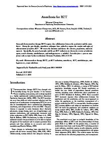
Figure 21 displays the mackerel egg density in the sampling area. The black hole in the upper right corner is caused by missing data in that area. Figure 21: Mackerel Egg Density



Figure 22: Predicted Mackerel Egg Density



In this example, the dependent variable is mackerel egg count, the independent variables are the geographical information about each of the sampling stations, and the logarithm of the sampling area is the offset variable. The following statements use the DIST=POISSON option to fit the nonparametric Poisson regression model: data mack2; set mackerel; log_net_area = log(net_area); run; proc adaptivereg data=mack2; model egg_count = longitude latitude depth distance / offset=log_net_area dist=poisson; output out=mackerelout p(ilink); run;



Figure 23 lists basic model information such as the offset variable, distribution, and link function. Figure 23 Model Information Mackerel Egg Density Study The ADAPTIVEREG Procedure Model Information Data Set Response Variable Offset Variable Distribution Link Function



16



WORK.MACK2 Egg_Count log_net_area Poisson Log



 SAS Global Forum 2013



Statistics and Data Analysis



Figure 24 lists fit statistics for the final model. Figure 24 Fit Statistics Fit Statistics GCV GCV R-Square Effective Degrees of Freedom Log Likelihood Deviance



6.94340 0.79204 29 -2777.21279 4008.60601



The final model consists of basis functions and interactions between basis functions for three geographic variables. Figure 25 lists seven functional components of the final model, including three one-way spline transformations and four two-way spline interactions. Figure 25 ANOVA Decomposition ANOVA Decomposition Functional Component



Number of Bases



DF



3 1 1 2 3 2 2



6 2 2 4 6 4 4



Longitude Depth Latitude Longitude Latitude Depth Distance Depth Latitude Depth Longitude



---Change If Omitted--Lack of Fit GCV 2035.77 420.59 265.05 199.17 552.75 680.45 415.77



3.3216 0.6780 0.4104 0.2496 0.8030 1.0723 0.6198



The “Variable Importance” table in Figure 26 displays the relative variable importance among the four variables. Longitude is the most important variable. Figure 26 Variable Importance Variable Importance



Variable



Number of Bases



Importance



7 8 5 3



100.00 30.26 18.93 8.56



Longitude Depth Latitude Distance



The following steps create and display in Figure 22 the predicted mackerel egg density over the spawning area: data mackplot; set mackerelout; pred = pred / net_area; run; proc sgrender data=mackplot template=surface; dynamic _title='Predicted Mackerel Egg Density' _z='pred'; run;



The graphs in Figure 21 and Figure 22 are quite similar.



17



 SAS Global Forum 2013



Statistics and Data Analysis



CONCLUSIONS The multivariate adaptive regression spline method of Friedman (1991), which is implemented in PROC ADAPTIVEREG, produces parsimonious models that do not overfit the data and thus have good predictive power. PROC ADAPTIVEREG can fit both linear and nonlinear nonparametric regression models. SAS/STAT software offers various tools for nonparametric regression, including the GAM, LOESS, and TPSPLINE procedures. Typical nonparametric regression methods involve a large number of parameters in order to capture nonlinear trends in data. Thus, the nonparametric model space is much larger than the parametric model space. The LOESS and TPSPLINE procedures are limited to problems in low dimensions. PROC GAM fits generalized additive models and can handle larger data sets than PROC LOESS and PROC TPSPLINE can handle. However, the additivity assumption ignores variable interactions in high-dimensional space, and convergence for nonnormal distributions is not guaranteed. PROC ADAPTIVEREG can fit models that these other procedures cannot fit. PROC ADAPTIVEREG is easy to use because it automatically selects the knots, creates the basis functions, performs the initial forward selection, and the final backward selection to generate the final model. Simple options enable you to train, test, validate, score, and predict new data.



SOFTWARE CREDITS The ADAPTIVEREG procedure was designed and programmed by Weijie Cai, Principal Research Statistician at SAS.



ACKNOWLEDGMENTS The authors are grateful to Anne Baxter, Funda Güne¸s, and Tim Arnold of SAS Institute Inc. for their valuable assistance in the preparation of this paper.



CONTACT INFORMATION Warren F. Kuhfeld SAS Institute Inc. S6018 SAS Campus Drive Cary, NC, 27513 (919) 531-7922 [email protected]



Weijie Cai SAS Institute Inc. S6048 SAS Campus Drive Cary, NC, 27513 (919) 531-0359 [email protected]



REFERENCES Asuncion, A. and Newman, D. J. (2007), “UCI Machine Learning Repository,” http://archive.ics.uci.edu/ml/. Bowman, A. W. and Azzalini, A. (1997), Applied Smoothing Techniques for Data Analysis, New York: Oxford University Press. Buja, A., Duffy, D., Hastie, T. J., and Tibshirani, R. (1991), “Discussion: Multivariate Adaptive Regression Splines,” Annals of Statistics, 19, 93–99. Friedman, J. H. (1991), “Multivariate Adaptive Regression Splines,” Annals of Statistics, 19, 1–67. Hastie, T. J., Tibshirani, R. J., and Friedman, J. H. (2001), The Elements of Statistical Learning, New York: SpringerVerlag.



SAS and all other SAS Institute Inc. product or service names are registered trademarks or trademarks of SAS Institute Inc. in the USA and other countries. ® indicates USA registration. Other brand and product names are trademarks of their respective companies. 18