International Capital Flows and Liquidity Crises Koralai Kirabaeva July 2009
Abstract This paper analyzes the composition of capital ‡ows (direct vs portfolio) between two countries in the presence of heterogeneity in liquidity risk and asymmetric information about the investment productivity. Direct investment is characterized by higher pro…tability and private information about investment productivity, while portfolio investment provides greater risk diversi…cation. I show that there is the possibility of multiple equilibria due to strategic complementarities in choosing direct investment. Further, I analyze the e¤ect of an increase in the liquidity risk in the host country on the composition of foreign investment. If there is a unique equilibrium then higher liquidity risk leads to a higher level of foreign direct investment (FDI). If, however, there are multiple equilibria, higher liquidity risk may lead to the opposite e¤ect: a decline of FDI in one of the equilibria. In this case, an out‡ow of FDI is induced by self-ful…lling expectations. The dual e¤ect of increased liquidity risk on capital ‡ows can be related to empirically observed patterns of foreign investment during liquidity crises. JEL classi…cation: G11, G15, D82
Correspondence: Financial Markets Department, Bank of Canada, Ottawa, ON, Canada K1A 0G9, E-mail:
[email protected]. I would like to thank David Easley, Karl Shell, and especially Assaf Razin for helpful comments and suggestions. I am also grateful to Levon Barsegyan, Ani Guerdjikova, Karel Mertens, Eswar Prasad, Viktor Tsyrennikov, and participants at Cornell - Penn State macroeconomics workshops. All errors are my own. The views expressed in this paper are those of the author. No responsibility for them should be attributed to the Bank of Canada.
1
1
Introduction
The two major types of international equity holdings are foreign direct investments (FDI) and foreign portfolio investments (FPI). Liquidity crises may be associated with an out‡ow of FPI and a simultaneous in‡ow of FDI, e.g., the 1994 crisis in Mexico and the late 1990s crisis in South Korea.1 This behavior re‡ects the …re-sale FDI phenomenon when domestic companies and assets are acquired by foreign investors at …re-sale prices. However, there is evidence that some liquidity crises have been accompanied by an out‡ow foreign investment, including FDI, e.g., the 2001 crisis in Argentina. Some theoretical literature argues that a liquidity crunch may induce and aggravate a real crisis, leading to an exit of foreign investors.2 The following question emerges: why during some liquidity crises is there an in‡ow of FDI while some others are accompanied by an out‡ow of FDI? In this paper, I develop a model which suggests an explanation of why FDI ‡ows exhibit such divergent behavior during liquidity crises. This paper presents a general equilibrium model which analyzes the composition of investment (direct vs portfolio) between two countries when there are heterogeneity in liquidity risk across countries and asymmetric information about the investment productivity. The characteristic feature of direct investment is concentrated ownership and control which provides access to private information about investment productivity3 and results in a more e¢ cient management.4 Portfolio investment represents holdings of assets which do not entail active management or control but allow for risk diversi…cation and greater liquidity. Taking advantage of the inside information, direct investors may sell low-productive investments and keep the high-productive ones under their ownership. This generates a "lemons"5 problem: the buyers do not know whether the investment is sold because of its low productivity or due to an exogenous liquidity shock. Therefore, due to this information 1
Krugman [24], Aguiar and Gopinath [4], Acharya, Shin, and Yorulmazer [1] Aghion, Bacchetta, and Banerjee [3], Chang and Velasco [11], and Caballero and Krishnamurthy [10]. 3 Klein, Peek, and Rosengren [23], Kinoshita and Mody [22], Bolton and von Thadden [9], Kahn and 2
Winton [20] 4 Due to the agency problem between managers and owners, portfolio investments are less e¢ cient (Goldstein and Razin [16]). 5 Akerlof (1970)
2
asymmetry, there is a discount on the prematurely sold direct investment (relative to the prematurely sold portfolio investment). This assumption is consistent with the evidence that there is a negative premium associated with seller-initiated block trades.6 The main implication of this information-based trade-o¤ is that the choice between direct and portfolio investment is linked to the likelihood with which investors expect to get a liquidity shock (Goldstein and Razin [16]). In my model, the agents have the Diamond-Dybvig [12] type preferences. Agents consume in period 1 or 2, depending on whether they receive a liquidity shock in period 1. The probability of an investor receiving a liquidity shock is country-speci…c. This probability captures the investor’s exposure to the liquidity shock; I will refer to it as the liquidity risk. In period zero, investors choose how much to invest into risky long-term projects in each of the two countries, as well as the ownership type for each project (direct or portfolio). In period one, idiosyncratic liquidity shocks are realized and, subsequently, risky investments are traded in the …nancial market. The late consumers are the buyers in the …nancial market. All investment projects pay o¤ in the second period. The equilibrium prices of direct and portfolio investments depend not only on their expected payo¤s but also on investors’ liquidity preferences and uncertainty about the investment productivity7 . If market is more liquid then expected gains from trading on private information are larger, since it is easier for informed traders to hide behind the liquidity traders.8 Therefore, in a more liquid market direct investors have higher pro…ts from selling on private information. On the other hand, a larger fraction of direct investors leads to a less liquid market. I show that there are two types of equilibria. In the …rst type, only investors from the country with a lower liquidity risk choose to hold direct investment. In the second type, investors from both countries hold direct investments. In this case, there are strategic 6
Holthausen, Leftwich, and Mayers [19], Easley, Kiefer and O’Hara [13], Easley and O’Hara [14], Keim
and Madhavan [21] 7 This is similar to the Allen and Gale ([6], [7]) "cash-in-the-market" framework where the market price is determined by the lesser of the following two amounts: expected payo¤ and the amount of safe asset available from buyers per unit of assets sold. 8 Easley and O’Hara [14], Kyle [25]
3
complementarities in choosing direct investment. This generates a possibility of multiple equilibria through the self-ful…lling expectations. If countries have the same fundamentals, the country with a higher liquidity risk attracts less inward foreign investment, but a larger share of it is in the form of FDI. Also, the country with a higher level of asymmetric information about investment productivity attracts more FDI relative to FPI since the marginal bene…ts from private information are larger. Further, I consider the e¤ect of an increase in the liquidity risk on the composition of foreign investment. Such an increase results in the drying up of market liquidity as more investors have to sell their risky asset holdings. At the same time, it becomes more likely that if a direct investment is sold before maturity, it is sold due to exogenous liquidity needs rather than an adverse signal about investment productivity. This reduces the adverse selection problem and therefore results in a smaller information discount on prematurely sold direct investments. This e¤ect captures the phenomenon of …re-sale FDI during liquidity crises. If economy is in the unique equilibrium then higher liquidity risk leads to a higher level of FDI. However, if there are multiple equilibria then FDI may decline as the liquidity risk increases. There are two possible interpretations of the liquidity risk in my model. One is the probability of a liquidity crisis that is unrelated to fundamentals of the economy. In fact, recent …nancial crises exhibit a large liquidity run component while the underlying macroeconomic fundamentals are not necessarily weak.9 Another interpretation is a measure of …nancial market development. In more developed …nancial (credit) markets it is easier for agents to borrow in case of liquidity needs, and therefore the probability of investment liquidation is smaller, whereas in developing and emerging countries access to the world capital markets is limited.10 So a country with a low liquidity risk can be viewed as a developed economy, and a country with a high liquidity risk can be viewed as a developing or emerging economy. In addition to a lower liquidity risk, a developed country can be characterized by a higher expected pro…tability (adjusted for risk) and less asymmetric information about the productivity. 9 10
Chang and Velasco [11] and Acharya, Shin, and Yorulmazer [2] Freedman and Click [15]
4
In the model, the dual e¤ect of an increase in the liquidity risk on the capital ‡ows corresponds to the empirically observed pattern of FDI during liquidity crises. The positive e¤ect of a higher liquidity risk on the inward FDI is consistent with the evidence documented by Krugman [24], Aguiar and Gopinath [4], and Acharya, Shin, and Yorulmazer [1]. Krugman [24] notes that the Asian …nancial crisis has been accompanied by a wave of inward direct investment. Furthermore, Aguiar and Gopinath [4] analyze data on mergers and acquisitions in East Asia between 1996 and 1998 and …nd that the liquidity crisis is associated with an in‡ow of FDI. Moreover, Acharya, Shin, and Yorulmazer [1] observe that FDI in‡ows during …nancial crises are associated with acquisitions of controlling stakes. At the same time, my model provides a possibility of a decrease in FDI through self-ful…lling expectations. This possibility is in line with the empirical evidence11 as well as theoretical literature that associates liquidity crises with an exit of investors from the crisis economy even if there are no shocks to fundamentals (Aghion, Bacchetta, and Banerjee [3], Chang and Velasco [11], and Caballero and Krishnamurthy [10]). My results are consistent with the empirical …ndings that countries that are less …nancially developed and have weaker …nancial institutions tend to attract more capital in the form of FDI12 . Moreover, my model can explain the phenomenon of bilateral FDI ‡ows among developed countries, and one-way FDI ‡ows from developed to emerging countries.13 The paper is organized as follows. Section 2 describes the related literature. Sections 3 and 4 present the theoretical model and its analysis. Sections 5 and 6 characterize the equilibrium. Sections 7 and 8 discuss the e¤ect of change in liquidity risk on the foreign investments. Section 9 concludes the paper. All proofs are delegated to the Appendix.
2
Related Literature
My paper is related to several papers in the literature. My model builds on the adverse selection property of FDI developed by Goldstein and Razin [16]. My model di¤ers from their model in several aspects. I examine the portfolio choice between two types of risky 11
Lipsey [26]. Albuquerque [5], Hausman and Fernandez-Arias [17] 13 Razin [29] 12
5
investment (direct vs portfolio) and safe asset in the two-country "cash-in-the-market" framework where investors have the Diamond-Dybvig [12] type of preferences (Allen and Gale [6] and Bhattacharya and Nicodano [8]). Goldstein and Razin [16] study the choice between FDI and FPI by risk-neutral investors in the partial equilibrium setting. They show that investors with higher liquidity needs are more likely to choose FPI over FDI. Also, they examine the implications of production costs, transparency in the host country, and heterogeneity of foreign investors in the source country. My model examines not only the composition of foreign investment but also the level thereof. My paper complements the results in Goldstein and Razin [16] by analyzing the bilateral investments ‡ows between two countries and, furthermore, the e¤ect of the change in liquidity preferences in the host country on inward foreign investment. In terms of addressing the …re-sale FDI phenomenon, this paper is related to Krugman [24], Aguiar and Gopinath [4], and Acharya, Shin, and Yorulmazer [1]. Krugman [24] points out the …re-sale FDI phenomenon and o¤ers two possible modeling approaches. One is based on moral hazard and asset de‡ation. The other explanation is based on disintermediation and liquidation, attributing the crisis to a run on …nancial intermediaries. Such a run can be set o¤ by self-ful…lling expectations. Aguiar and Gopinath [4] propose a model where foreign investors have …nancial resources to acquire domestic assets and superior technology. Acharya, Shin, and Yorulmazer [1] address the …re-sale FDI phenomenon from the …rm’s prospective. They provide an agency-theoretic framework in which during the crisis, the loss of control by domestic managers together with the lack of domestic capital result in a transfer of ownership to foreign …rms. This paper o¤ers an alternative explanation of the …re-sale FDI phenomenon based on the adverse selection. In contrast to the explanations above, in my model a liquidity crisis may lead to a decline in FDI (through self-ful…lling expectations). The following papers link …nancial crises and liquidity through models of self-ful…lling creditors’run. Chang and Velasco [11] place international illiquidity at the center of …nancial crises. They argue that a small shock may result in …nancial distress, leading to costly asset liquidation, liquidity crunch, and large drop in asset prices. Caballero and Krishnamurthy [10] argue that during a crisis self-ful…lling fears of insu¢ cient collateral may trigger a
6
capital out‡ow.
3
Model
I consider a model with 2 countries: A and B. There is a continuum of agents with an aggregate Lebesgue measure of unity. Let
be the proportion of investors living in country
A; and the rest of the investors live in country B. There are 3 time periods: t = 0; 1; 2: There is only one good in the economy, and in period zero, all agents are endowed with one unit of good that can be consumed and invested.
3.1
Investment technology
Agents have access to two types of constant returns technology. One is a storage technology (safe asset), which has zero net return: one unit of safe asset pays out one unit of safe asset in the next period. The safe asset is the same in both countries, and I will refer to it as "cash." The other type of technology is a long-term risky investment project (also called risky asset). In period two, the risky investment in project i has a random idiosyncratic payo¤
0
1
2
safe asset
1!
1!
1
investment
1!
0!
Figure 1. Payo¤ structure.
The investment productivity of each project
2) k
with mean Rk and variance
2 .14 k
The produc-
tivity mean Rk is a random variable that takes two values: a low value Rkl with probability 14
More precisely, all portfolio investments have the same productivity mean Rpk , and all direct investments
have the same productivity mean Rdk > Rpk , as discussed in Section 3.3
7
k
15 k) .
and a high value Rkh with probability (1
(For each investment project in coun-
try k; nature picks the mean Rk where Rk 2 fRkl ; Rkh g.)16 The expected productivity mean is denoted by Rk =
k Rkl
+ (1
k ) Rkh
with Rk > 1. All parameters of the pro-
ductivity distribution are country-speci…c, with Rk representing the expected pro…tability 2 k
of investment project and
capturing the investment risk in country k.
Agents can invest their endowment in investment projects at home (domestic investment) and abroad (foreign investment). The holdings of the two-period risky investment can be traded in …nancial market at date t = 1.
3.2
Preferences
Agents consume in period 1 or 2, depending on whether they receive a liquidity shock in period 1. The probability of receiving a liquidity shock in period one is country-speci…c: investors in each country k 2 fA; Bg have the same probability
k.
This probability (
k)
captures the liquidity risk in a given country. Investors who receive a liquidity shock have to liquidate their risky long-term asset holdings and consume all their wealth in period one. So they are e¤ectively early consumers who value consumption only at date t = 1. The rest are the late consumers who value the consumption only at date t = 2. Since there is no aggregate uncertainty,
k
is also a fraction of investors hit by a liquidity shock in country
k. Investors from country k have Diamond-Dybvig type of preferences: Uk (c1 ; c2 ) =
k u(c1 )
+ (1
k )u(c2 )
(1)
where ct is the consumption at dates t = 1; 2. In each period, investors have mean-variance utility E [u(ct )] = E [ct ] 15
In addition, the probability
k
2
Var [ct ]
(2)
of investment project to be less productive depends on the type of
ownership:the direct investment is less likely to have low mean productivity than the portfolio investment, i.e., 16
dk < pk (discussed in Section 3.3). Informed investors are able to observe the true distribution, uninformed investors use the unconditional
distribution which the mixture of two normal distributions.
8
with
representing the degree of risk aversion17 . Investors choose their asset holdings to
maximize their expected utility. Without loss of generality, I assume that country A has a smaller liquidity risk than country B, i.e.,
3.3
A
<
B.
Direct and Portfolio Investments
In period t = 0, agents decide how much of their endowment to invest in long-term risky investment projects. In a given country k, an agent can either invest directly in a single project, or become a portfolio investor investing in up to Nk projects.18 Direct investors are able manage projects more e¢ ciently, therefore, the productivity of direct investment is more likely to be drawn from a high mean distribution than the productivity of portfolio investment, i.e.,
dk
<
pk .
Therefore, the expected pro…tability of
a direct investment Rdk is higher than the expected pro…tability of a portfolio investment (Rpk ) per unit of investment. Furthermore, in period one, direct investors in country k observe a signal about their investment productivity: the true value of productivity mean Rdk . Henceforth, I will refer to it as the productivity signal. Portfolio investors do not observe such productivity signal. Therefore, portfolio investors use the updating on the productivity mean in country k: Rpk =
pk Rkl +(1
pk ) Rkh .
The decision to become direct or portfolio investor is country-
speci…c, i.e., it is possible to be a direct investor in one country, and a portfolio investor in another. The advantage of direct investment is private information about the idiosyncratic investment productivity. However, it is public knowledge which investors are informed. This generates the adverse selection problem: it is not known whether direct investors sell due to a liquidity shock or because they have observed the negative productivity signal (high 17
Maccheroni, Marinacci, and Rustichini [27] show that the mean-variance preferences is the special case
of variational preferences, which is a representation of preferences for decision making under uncertainty. The mean-variance preferences have been used in the …nance literature, for example, Van Nieuwerburgh and Veldkamp (2008). 18 Due to the mean-variance preferences and idiosyncratic productivity, a portfolio investor will always choose to invest into the maximum number of projects allowed.
9
variance). Therefore there is an information discount on the price of direct investment at t = 1. In this setting, the e¢ ciency of direct over portfolio investment is re‡ected by higher expected productivity of the former: Rdk > Rpk . Also, the diversi…cation bene…ts from portfolio investment are captured by allowing to invest in multiple projects in one country, which is e¤ectively equivalent to reducing the investment variance by the factor of Nk . I abstract from the other gains of management control such as possibility of restructuring19 that may lead to an increase of investment payo¤ from t = 1 to t = 2. In period one, the liquidity shocks are realized, direct investors observe a signal about the productivity of their investments, and trading in …nancial market occurs. Investors who receive a liquidity shock supply their asset holdings inelastically. In addition, direct investors who have not received a liquidity shock but observe a negative productivity signal can sell their investments. The buyers are investors who have not received a liquidity shock in period one. Figure 2 represents the time line of the model.
Figure 2. Time line. I show that the decision between direct and portfolio investment depends on the probability of getting a liquidity shock and uncertainty about the investment productivity. Agents are more likely to choose direct investment if they are less likely to receive a liquidity shock.
4
Investors’decision problem
Agents face the following two-stage decision problem. At date t = 0, an agent decides whether to become a direct or a portfolio investor in each country and, correspondingly, 19
The trade-o¤ between e¢ ciency gains related to corporate control and liquidity have been addressed by
Bolton and von Thadden [9], Maug [28], and Holmstrom and Tirole [18].
10
how much of their endowment to invest in the risky long-term projects. At date t = 1; investors who have not received a liquidity shock, decide how much of the long-term assets they want to buy.
Figure 3. Investors’decision problem In period one, investors are restricted to buying either direct or portfolio investment in each country. This assumption is imposed to prevent further risk diversi…cation. Therefore, in the equilibrium a buyer should be indi¤erent between buying direct or portfolio investment in a given country. Note that at period t = 1 there is no advantage of private information. Let
ik
2 [0; 1] be the fraction of direct investors from country i investing in country
k where i; k 2 fA; Bg. Then the fraction of direct investors investing in country k is k
=
Ak
+ (1
)
Bk .
The investor who buys a risky asset from a direct investor in period t = 1, does not know whether it is sold due to the liquidity shock or because of the low productivity mean. Buyers believe that direct investors in country k will receive a liquidity shock with probability dk
=
+ (1 Ak + (1
Ak A
Therefore, the buyers believe that with probability
) )
Bk B
.
(3)
Bk dk
dk +(1
dk ) dk
try k is sold due to a liquidity shock, and with probability
direct investment in coun-
(1 dk ) dk dk +(1 dk ) dk
it sold because
its low productivity. Hence, buyers believe that the productivity mean of the asset sold
11
by a direct investor is low Rkl with probability bility
dk dk +(1
dk ) dk
(1 dk +(1
dk ) dk dk ) dk
and high Rkh with proba-
. Using Bayesian updating, the mean of the prematurely sold direct
investment in country k is
and its variance is
bdk R
(1 dk + (1
dk ) dk dk )
Rkl + dk
d d + (1
d)
Rkh ;
(4)
2. k
Portfolio investors do not observe a productivity signal, hence they only sell their investment if they are hit by a liquidity shock. Therefore, the productivity of the prematurely sold portfolio investment in country k has mean Rpk and variance
2 =N . k k
Since investment
productivity is idiosyncratic, there is no updating on the productivity variance of portfolio investment based on the direct investors selling. Several assumptions are imposed on the parameters Rkl ; Rkh ;
2; k
dk ;
pk ; Nk
of the
productivity distribution for each country k 20 : Assumption 1. In the absence of private information, investors are indi¤erent between holding direct and portfolio investment. This assumption implies that bene…ts from diversi…cation are perfectly o¤set by bene…ts from management e¢ ciency resulting in the higher expected productivity. Assumption 2. At t = 0, all investors invest some but not all of their endowment in risky projects. Assumption 3. At t = 1, investors’demand for risky assets in both countries is less than his safe asset holdings. The investors from country i 2 fA; Bg choose their optimal investment holdings in each country k 2 fA; Bg at date t = 0 to maximize their expected utility. Denote by xidk the demand for direct investment at t = 0 by an investor from country i. Similarly, denote by xipk the total demand for portfolio investment at t = 0 by an investor from country i (this demand is divided equally among Nk projects). At date t = 1, uncertainty about the liquidity shock is resolved and all investors observe the total proportion of early consumers, however, their identity is private information. Denote the prices of direct and portfolio investments in country k 2 fA; Bg by ppk and pdk , 20
See Appendix A.1
12
respectively. Let ypk and ydk be the demand for direct and portfolio investment in country k in period one. Since the liquidity shock is realized at date t = 1, the demands ypk and ydk are the same for investors from both countries (so superscript i can be omitted).21 The demand for direct and portfolio investments in period one are given by Rpk
ypk =
ppk 2 =N k k
bdk R
ydk =
(5)
pdk 2 k
where k 2 fA; Bg22 . Since investors are restricted to buying either only direct or only portfolio investment at t = 1 in a given country k, the optimal demand for the risky asset is given by yk = max fydk ; ypk g. The optimal demand for the portfolio investment in country k by an investor from country i in period t = 0 is given by
xipk =
Rpk
1
i
(1
i)
Rpk ppk 2 =N k k
(6)
The optimal demand for the direct investment in country k by an investor from country i in period t = 0 is given by
xidk =
(Rkh
1) (1
i (Rkh 2 i) k
pdk )
(7)
Note that the demand for risky investment (both direct and portfolio) at t = 0 is a decreasing function of liquidity risk ( i ), i.e., investors from a country with a lower liquidity risk will allocate a larger fraction of their endowment to risky assets in period zero. Also, the demand for risky investment is an increasing function of the price of the investment at t = 1., i.e., agents will invest a larger amount of their endowment into risky projects if the re-sale price in the next period is higher. 21
The demand for risky asset at t = 1 is independent from investment demand at t = 0 due to the mean-
variance preferences and assumption 2. Since after the realization of liquidity shock, the survived investors A B from both countries are identical, and their demands for each type of the risky asset is the same: ypk = ypk A B and ydk = ydk . 22 See Appendix A.2 for maximization problem.
13
5
Equilibrium
Recall that
ik
2 [0; 1] denotes the fraction of direct investors from country i investing in
country k, where i; k 2 fA; Bg. Given the fractions (
ik
: i; k 2 fA; Bg) of direct investors in the economy, prices (ppk ; pdk )
and demand functions xipk ; xidk ; yk
for all i; k 2 fA; Bg, constitute a Rational Expecta-
tions Equilibrium (REE) if (i) xidk ; yk (respectively, (xipk ; yk )) maximizes the expected utility of a direct (respectively, portfolio) investor i, given the prices (pdk ; ppk ) and (ii) the market for investments clears at t = 1. The overall equilibrium in the economy is given by
i i ik ; (pdk ; ppk ) ; (xdk ; xpk ; yk )
for
i; k 2 fA; Bg.
5.1
Properties of Equilibrium
Property 1. In an equilibrium, the prices satisfy pdk
1 and ppk
1.
If the price of direct investment in country k is greater than one then agents will invest all of their endowment in this country. Then there is no safe asset holding in period one, therefore pdk > 1 cannot be an equilibrium price. Similarly, for portfolio investment. Property 2. In an equilibrium, the optimal demands for portfolio and direct investments are equal:
bdk R
pdk 2 k
=
Rpk
ppk 2 =N k
(8)
Given the assumption that investors can buy only one type of asset in each country, the expected utilities of buying direct and portfolio investments in period one should be equal in the equilibrium. Otherwise, all investors will buy only the type of investment which yields higher expected utility. Property 3. In an equilibrium, a direct investor sells his investment if he observes a negative productivity signal. Suppose a direct investor does not sell his investment after observing a negative signal. Then by Assumption 3, ex-ante the investor is better o¤ by choosing the portfolio investment at t = 0 since he can sell it for a higher price at t = 1 in case of a liquidity shock.
14
The equilibrium prices of direct investment (pdk ) and portfolio investment (ppk ) are determined by equation (7) and the market clearing condition (8). 0
( (1
A)
+ (1
) (1
Ak
(
B B B + (1 B B )) yk = B B + (1 @ + (1
A
)
+ (1 Bk Ak )
) (1
A)
(
B
A k ) xdk
+ (1
B)
B k ) xdk
A A xpk Bk )
B B xpk
1 C C C C C C A
(9)
In each country k, risky investment is supplied by the agents who received a liquidity shock or the adverse signal about investment productivity. The buyers are the agents who have not received a liquidity shock.
5.2
Choice between direct and portfolio investments
In period t = 0, an investor from country i chooses to become a direct investor in country k only if his expected utility from holding direct investment is greater than or equal to his expected utility from holding portfolio investment: EU xidk
EU xipk . If the
two utilities are equal then an investor is indi¤erent between holding direct or portfolio investment. Recall that the liquidity risk in country A is less than in country B:
A
<
B:
Lemma 1. For any country k 2 fA; Bg, if some investors from country B hold direct investment in country k, i.e., investment in country k, i.e.,
Ak
Bk
> 0, then all investors from country A hold direct
= 1.
Lemma 1 follows from the fact that the demand for risky investment is a decreasing function in liquidity risk. This lemma implies that if some investors from country A (but not all) choose to hold direct investment in country k, then none of the investors from country B hold direct investment in that country. In particular, if for investors from country A the expected utility from holding direct investment is less than the expected utility from holding portfolio investment, then only portfolio investments will be held in equilibrium. Proposition 1 For each country k 2 fA; Bg, there are two possible types of equilibria. In type I,
Ak
2 [0; 1) and
Bk
= 0, i.e., only investors from country A (but not all) hold direct 15
investment; the equilibrium of this type is unique. In type II,
Ak
= 1 and
Bk
2 [0; 1], i.e.,
all investors from country A hold direct investment; there are at most three such equilibria. Type I equilibrium includes the (corner) equilibrium with portfolio investments only and a pooling equilibrium for investors from country A. The equilibrium of type I is unique because there is a strategic substitutability in becoming a direct investor. Therefore, there is a unique equilibrium
Ak
such that if the proportion of direct investors is below
A then EU xA dk > EU xpk ; and if the proportion of direct investors is above
Ak
Ak
then
A EU xA dk < EU xpk .
Type II equilibrium includes the (corner) equilibrium with direct investments only, a pooling equilibrium for investors from country B, and the separating equilibrium where direct investments are held by investors from country A and portfolio investments are held by investors in country B. The multiplicity of type II equilibria is based on the e¤ect of expectations on the price of prematurely sold direct investment. On one hand, similarly to the type I equilibrium, as the fraction of direct investors
Bk
increases, the price of direct investment goes down in
country k, decreasing the bene…ts from holding direct investment. On the other hand, the information discount on the price of direct investment depends on the probability of direct investors selling due to the negative productivity signal. If there are more direct investors with a high liquidity risk then the market believes that the probability of a direct investor selling due to a liquidity shock is higher and, therefore, the price discount on the prematurely sold direct investment is smaller. So, more investors from country B choose to hold direct investment if they believe that other investors from country B are holding direct investment. This strategic complementarity among direct investors generates multiple equilibria. If there are two or three equilibria then one of the equilibria is a separating equilibrium where all investors with a low liquidity risk hold direct investment, and all investors with a high liquidity risk hold portfolio investment. Overall, there are …ve possible cases of composition of direct and portfolio investment that can occur in the equilibrium in a given country: 1. investors from both countries hold portfolio investments;
16
2. some investors from country A hold direct investments and others hold portfolio investments; 3. all investors from country A hold direct investments and all investors from country B hold portfolio investments; 4. some investors from country B hold portfolio investments and others hold direct investments; 5. investors from both countries hold direct investments. Figures 4 illustrates the possible equilibria regions for di¤erent values of such that
A
<
B.
Each point in the (
A;
B)
A
and
B
plane corresponds to a particular case of
equilibria in the enumeration above, except for the points with multiple equilibria (when cases 3 and 4 occur simultaneously). Thus, each type corresponds to a region in the plane; these regions are colored distinctly and numbered accordingly. We consider three examples with the same values of Rh = 1:2; Rl = 0:9; values of
2
= 0:1;
p
=
d
= 0:5; N = 1 and di¤erent
(the fraction of investors in country A). Note that as
becomes larger the area
with multiple equilibria disappears.
Figure 4
6
Possible equilibria regions for di¤erent values of
A
and
B
Composition of Foreign Investment
De…ne the foreign direct investment from country A to country B as the holdings of direct investment in country B by investors from country A: FDI AB =
A A xdB .
Similarly, de…ne
the foreign portfolio investment from country A to country B as the holdings of portfolio 17
investment in country B by investors from country A: FPI AB = foreign investment from country A to country B is FI AB =
A A ) xpB .
(1
A A xdB +
(1
Then the
A A ) xpB .
De…ne
FDI BA , FPI BA , and FI BA similarly. There are two dimensions in which the two countries may di¤er. One is the liquidity risk (
k ),
another is the distribution parameters of investment productivity that represent
the country’s fundamentals: Rkl ; Rkh ;
2; k
dk ;
pk ; Nk
.
There are two possible interpretations of liquidity risk in my model. One is the probability of a liquidity crisis that is unrelated to fundamentals of the economy. Another is a measure of …nancial market development: in more developed …nancial markets it is easier for agents to borrow in case of liquidity needs, therefore the probability of investment liquidation is smaller. Accordingly, a country with a low liquidity risk can be viewed as a developed country, and a country with a high liquidity risk can be viewed as a developing or emerging economy. Suppose the countries di¤er only in terms of liquidity risk and are identical with respect to productivity parameters. In this case, the country with a higher liquidity risk attracts less foreign investment, but a higher share of it in the form of FDI. Figures 5 illustrates the possible compositions of bilateral investment holdings in the di¤erent types of equilibria. 5a. Type I pooling equilibrium 5b. separating equilibrium 5c. Type II pooling equilibrium
Figure 5. Bilateral investment holdings in di¤erent types of equilibria. In addition to a lower liquidity risk, a developed country can be characterized by a higher expected payo¤ (adjusted for risk) and smaller bene…ts from private information of FDI. Property 4.
In an equilibrium, the share of FDI from country i to country k is
higher if either of the following holds: (i) e¢ ciency gains of direct investment Rdk are larger, (ii) uncertainty about investment productivity (Rkh
Rpk
Rkl ) is larger, (iii) risk
diversi…cation opportunities (Nk ) are smaller. Both FDI and FPI holdings are larger if in the host country the expected pro…tability 18
is higher and the investment risk is lower. The larger uncertainty about investment productivity positively a¤ects the share of direct investments relative to portfolio investments since the bene…ts from private information are larger. If direct investment is more e¢ cient relative to portfolio investment, then the share of direct investments is higher, which corresponds to higher equilibrium levels of
Ak
and
Bk .
On the other hand, larger diversi…cation
bene…ts from portfolio investment result in a smaller share of FDI. My results are consistent with the empirical …ndings that countries that are less …nancially developed and have weaker …nancial institutions tend to attract more capital in the form of FDI. This o¤ers a liquidity-based explanation of the phenomenon of bilateral FDI ‡ows among developed countries and one-way FDI ‡ows from developed to emerging countries. Moreover, Freedman and Click [15] show that banks in developing countries maintain a high level of liquid assets, while allocating only a modest amount of funds to productive businesses through loans. They argue that this di¤erence among developed and developing countries is due to ine¢ ciencies in credit markets resulting from factors such as greater macroeconomic risk and signi…cant de…ciencies in the legal and regulatory environment.
7
Liquidity risk
In this section, I study the e¤ect of change in the liquidity risk ( ) on investment holdings in each country. First, I examine how the composition of foreign investment is a¤ected by an increase in the liquidity risk in the host country.(comparative statics). Next, I introduce aggregate uncertainty about liquidity risk and analyze how the investment holding and prices are a¤ected.
7.1
Comparative Statics
In this section, I analyze how the composition of foreign investment is a¤ected by an increase in the liquidity risk in the host country. Consider country A as a host country and country B as a source country. Suppose country A is in the type II pooling equilibria with respect to inward foreign investment,
19
that is, it has in‡ows of both FDI and FPI. In this case, an increase in the liquidity risk in the host country (
A)
leads to a lower level of total foreign investment. The e¤ect on
the composition of foreign investment is ambiguous and depends on the equilibrium. If economy is in the unique equilibrium then an increase in
A
leads to more FDI and less
FPI. However, if there are multiple equilibria then FDI may increase or decrease depending on the equilibrium. As the liquidity risk increases, two e¤ects take place. First, market liquidity is reduced re‡ecting the higher preference for safe liquid asset. This leads to lower level of foreign investment including FDI. At the same time, it reduces the adverse selection problem associated with direct investments: the fraction of FDI “lemons” is lower. This results in a smaller information discount on direct investment, and therefore, leads to a higher level of FDI. If there are multiple equilibria and the economy is in the equilibrium with a larger fraction of direct investors (
BA )
or if the equilibrium is unique, then the second e¤ect
dominates and an increase in liquidity risk in the host country leads to a higher level of FDI. If the economy is in the equilibrium with a smaller fraction of direct investors (
BA )
then the …rst e¤ect dominates and, therefore, an increase in liquidity risk in the host country leads to a lower level of FDI. In this case, the out‡ow of FDI is associated with self-ful…lling expectations: if an agent expects less agents to hold direct investments, then he chooses not to hold direct investment himself. A similar argument applies to the case when country B is a host country. These results are summarized below. Proposition 2 Suppose country k 2 fA; Bg is in type II pooling equilibrium with respect to inward foreign investment. Then (i) if there is a unique equilibrium then an increase in liquidity risk results in a higher level of FDI; (ii) if there are multiple equilibria then an increase in liquidity risk results in a higher level of FDI in one equilibrium, and a lower level of FDI in another.
20
7.2
Aggregate uncertainty about liquidity risk
Suppose there are two aggregate liquidity states ( <
kL
kH .
The state
kH
kL ;
kH )
for the host country k such that
is a crisis state where the fraction of investors hit by a liquidity
shock is larger. These states are realized with ex-ante probabilities (1
q) and q. Suppose
country A is facing aggregate uncertainty about the liquidity risk, therefore, there are two aggregate states: a normal state SL = ( AH
>
AL ;
B)
and a crisis state SH = (
AH ;
B)
where
AL .
All investment decisions at t = 0, such as fractions of direct investors (
Ak ; Bk )
and
A B B direct and portfolio investment holdings xA dk ; xpk ; xdk ; xpk , are made before liquidity state
S is realized. However, it a¤ects the prices and demands for direct and portfolio investments in period one depend on which state is realized. There are two ways in which the prices are a¤ected, one is through the market liquidity and another is through the adverse selection problem associated with direct investment. The …rst e¤ect is the dry up of market liquidity as more investors have to sell their asset holdings, and fewer investors are buying. Therefore, investment prices fall in order to clear the market. At the same time, direct investments are more likely to be sold before maturity due to a liquidity shock rather than because of the adverse productivity signal. Therefore, the market belief about the probability of receiving a liquidity shock (
d)
is higher than
in a crisis state relative to a normal state. This reduces the adverse selection problem and results in a smaller information discount on direct investment. Then the depressed prices together with the reduced discount on direct investment capture the phenomenon of …re-sale FDI. The lower prices re‡ect the di¢ culty of …nding buyers during the crisis. Aguiar and Gopinath [4] show that during the Asian …nancial crisis in late 1990s the median ratio of o¤er price to book value substantially declined. The low liquidity of domestic investors led to the signi…cant increase in acquisitions involving foreign investors. Next suppose that probability of a crisis depends on the previously realized state. So that conditional probability of transition from a normal state to a crises state is smaller than the conditional probability of remaining in a crisis state. The transition matrix is
21
2
1
qLH
qLH
3
5 where qHH > qLH . 1 qHH qHH Then we can compare the equilibria sequentially, and analyze how the composition
given by 4
of foreign investment depends on the expectation of a liquidity crisis. Similarly to the comparative statics with respect to an increase in liquidity risk, a higher expectation of a liquidity crisis has two e¤ects. One is reduced market liquidity since investors’preferences for liquidity are higher. Another is a smaller information discount on the prematurely sold direct investment. The …rst e¤ect leads to less FDI while the second e¤ect results in more FDI. If there is a unique equilibrium, then second e¤ect (reduced adverse selection) dominates so higher liquidity risk leads to a higher level of FDI. If, however, there are multiple equilibria, higher liquidity risk may lead to a lower level of FDI. Figure 6 illustrates the e¤ect of an increase in probability of a liquidity crisis q on foreign direct and portfolio investment in the case of multiple equilibria. The solid and dotted lines depict the changes in equilibrium investment values as the probability of a liquidity crisis q increases.
0.2
0.05 0
0
0.5
FDI+FPI
0.1
FPI
FDI
0.2 0.1 0
0
0.5
q
0.19 0.18 0
q
0.5 q
Figure 6. FDIBA and FPIBA as functions of s The results can be related to the empirically observed pattern of FDI during liquidity crises, as discussed in the following section.
22
8
Empirical evidence
In this section, I consider the empirical data on foreign investment during the episodes of liquidity crises. The capital ‡ows data is from the Lane and Milesi-Ferretti (2006) dataset.23 On one hand, the positive e¤ect of a higher liquidity risk on the inward FDI is consistent with the evidence of …re-sale FDI. Figure 7 shows the FDI and FPI ‡ows into South Korea and Mexico in the time period around their respective …nancial crises in late 1990s and 1994.24
x 10
Kore a
4
x 10
10
FD I
FD I
FPI
FPI
FI
FI
10
5
5
0 1998
M e x ic o
4
15
15
1999
2000
0 1992
2001
1993
1994
1995
1996
1997
1998
Figure 7. Crises in Korea and Mexico: in‡ow of FDI and out‡ow of FPI (millions of 2006 U.S. dollars). Both Korea and Mexico can be viewed as a country B (a country with higher liquidity risk) in my model, and the …nancial crises can be interpreted as the increase in liquidity risk
B.
Then, according to my model, if a country is in type I equilibria with respect to
inward foreign investment, then the higher liquidity risk leads to more FDI and less FPI. If a country is in type II equilibria with respect to inward foreign investment, then an increase in liquidity risk results in a higher level of FDI in one of the equilibria. As we can see from the …gure, in Korea during the late 1990s crisis and in Mexico following the 1994 crisis the FDI level has been increasing while FPI level has declined. 23
They construct estimates of external assets and liabilities, distinguishing between foreign direct invest-
ment, portfolio equity investment, o¢ cial reserves, and external debt for over 140 countries over the period of 1970-2004. 24 The East Asian …nancial crisis started in Thailand with the …nancial collapse of the Thai baht in 1997. Indonesia, South Korea, Malaysia, and the Philippines were the most a¤ected by the crisis. The Mexican (Tequila) crisis was triggered by the sudden devaluation of the Mexican peso in December, 1994.
23
Furthermore, the insurge of FDI during liquidity crises is supported by empirical evidence on mergers and acquisitions in crises-stricken countries. Analyzing …rm-level dataset on mergers and acquisitions in countries that underwent the Asian …nancial crises in late 1990s, Aguiar and Gopinath [4] …nd that during the crisis foreign acquisitions increased by 91% while domestic acquisitions declined by 27%. Moreover, Acharya, Shin, and Yorulmazer [1] observe that FDI in‡ows during …nancial crises are associated with acquisitions of stakes that grant control and, furthermore, the assets acquired in …re sales are subsequently re-sold quickly (‡ipped) to domestic buyers once the crisis has past. On the other hand, my model provides a possibility of a decrease in FDI through selfful…lling expectations. This possibility is consistent with the behavior of FDI during the early 1990s crisis in Sweden25 and the 2001 crisis in Argentina26 . As …gure 8 shows, FDI has declined in both countries.
x 10
4
S w e de n
x 10
6
Arge ntina
4
10 FD I
5 4
FD I
FPI
8
FPI
FI
FI
6 3 4
2
2
1 0 1990
1991
1992
0 2000
1993
2001
2002
2003
2004
Figure 8. Crises in Sweden and Argentina: out‡ow of FDI (millions of 2006 U.S. dollars). Sweden can be viewed as a country A. Suppose it is in the type II pooling equilibria with respect to inward foreign investment, that is, it has in‡ows of both FDI and FPI. If there are multiple equilibria then an increase in
A
may leads to less FDI and more FPI
depending on the equilibrium. Argentina can be viewed as a country B. If it is in type II equilibria with respect to inward foreign investment, then it has in‡ows only of FDI. Then an increase in the country liquidity risk 25 26
B
may result in a lower level of FDI in one of the equilibria. The level of
The Exchange Rate Mechanism crisis in Scandinavia in early 1990s. Argentina defaults in December 2001.
24
FPI into Argentina in early 2000s is almost at zero.
9
Conclusion
I analyze the composition of foreign investment between two countries which may di¤er in two dimensions: liquidity risk (probability of a liquidity crisis) and the investment productivity (fundamentals). I show that the country with a higher liquidity risk attracts less foreign investment, but a higher share of it is in the form of FDI. Also, a country with a larger investment risk attracts more FDI relative to FPI since the marginal bene…ts from private information are larger. This is consistent with the empirical …ndings that countries that are less …nancially developed attract more capital in the form of FDI. Furthermore, these results o¤er an explanation based on the di¤erence in liquidity risk for the phenomenon of bilateral FDI ‡ows among developed countries and one-way FDI ‡ows from developed to emerging countries. The e¤ect of an increase in liquidity risk in the host country on FDI is ambiguous. If the economy is in the unique equilibrium then a higher liquidity risk leads to larger FDI holdings and smaller FPI holdings. This result is in line with the …re-sale FDI phenomenon. If, however, there are multiple equilibria then a higher liquidity risk may lead to the opposite e¤ect: FDI declines. In this case, an out‡ow of FDI is induced by self-ful…lling expectations. This dual impact of increased liquidity risk on foreign investment consistent with empirical evidence on capital ‡ows during liquidity crises.
25
References [1] V. Acharya, H. Shin, and T. Yorulmazer. Fire-sale FDI. Working Paper (2007). [2] V. Acharya, H. Shin, and T. Yorulmazer. Fire Sales, Foreign Entry and Bank Liquidity. Working Paper (2007). [3] P. Aghion, P. Bacchetta, and A. Banerjee. A simple model of monetary policy and currency crises. European Economic Review 44(4-6) (2000). [4] M. Aguiar and G. Gopinath. Fire-Sale Foreign Direct Investment and Liquidity Crises. The Review of Economics and Statistics 87(3), 439–52 (2005). [5] R. Albuquerque. The composition of international capital ‡ows: risk sharing through foreign direct investment. Journal of International Economics 61(2), 353–383 (2003). [6] F. Allen and D. Gale. Limited Market Participation and Volatility of Asset Prices. The American Economic Review 84(4), 933–955 (1994). [7] F. Allen and D. Gale. Financial intermediaries and markets. Econometrica pp. 1023–1061 (2004). [8] S. Bhattacharya and G. Nicodano. Insider Trading, Investment, and Liquidity: A Welfare Analysis. The Journal of Finance 56(3), 1141–1156 (2001). [9] P. Bolton and E. von Thadden. Blocks, Liquidity, and Corporate Control. The Journal of Finance 53(1), 1–25 (1998). [10] R. Caballero and A. Krishnamurthy. International and domestic collateral constraints in a model of emerging market crises. Journal of Monetary Economics 48(3) (2001). [11] R. Chang and A. Velasco. A Model of Financial Crises in Emerging Markets*. Quarterly Journal of Economics 116(2) (2001). [12] D. Diamond and P. Dybvig. Bank Runs, Deposit Insurance, and Liquidity. The Journal of Political Economy 91(3), 401–419 (1983). 26
[13] D. Easley, N. Kiefer, and M. O’Hara. The information content of the trading process. Journal of Empirical Finance 4(2-3), 159–186 (1997). [14] D. Easley and M. O’Hara. Price, trade size, and information in securities markets. Journal of Financial Economics 19(1), 69–90 (1987). [15] P. Freedman and R. Click. Banks That Don’t Lend? Unlocking Credit to Spur Growth in Developing Countries. Development Policy Review 24(3), 279–302 (2006). [16] I. Goldstein and A. Razin. An information-based trade o¤ between foreign direct investment and foreign portfolio investment. Journal of International Economics 70(1), 271–295 (2006). [17] R. Hausmann and E. Fernandez-Arias. Foreign Direct Investment: Good Cholesterol? Foreign Direct Investment Versus Other Flows to Latin America (2001). [18] B. Holmstrom and J. Tirole. Market Liquidity and Performance Monitoring. The Journal of Political Economy 101(4), 678–709 (1993). [19] R. Holthausen, R. Leftwich, and D. Mayers. The E¤ect of Large Block Transactions on Security Prices: A Cross-sectional Analysis. Journal of Financial Economics 19(2), 237–267 (1998). [20] C. Kahn and A. Winton. Ownership Structure, Speculation, and Shareholder Intervention. The Journal of Finance 53(1), 99–129 (1998). [21] D. Keim and A. Madhavan. The upstairs market for large-block transactions: analysis and measurement of price e¤ects. Review of Financial Studies 9(1), 1–36 (1996). [22] Y. Kinoshita and A. Mody. Private information for foreign investment in emerging economies. Canadian Journal of Economics 34(2), 448–464 (2001). [23] M. Klein, J. Peek, and E. Rosengren. Troubled banks, impaired foreign direct investment: the role of relative access to credit. American Economic Review 92(3), 664–682 (2002).
27
[24] P. Krugman. Fire-Sale FDI. Capital Flows and the Emerging Economies: Theory, Evidence and Controversies, Chicago pp. 43–60 (2000). [25] A. Kyle. Market Structure, Information, Futures Markets, and Price Formation. International Agricultural Trade: Advanced Readings in Price Formation, Market Structure, and Price Instability pp. 45–64 (1984). [26] R. Lipsey. Foreign Direct Investors in Three Financial Crises. NBER Working Paper (2001). [27] F. Maccheroni, M. Marinacci, and A. Rustichini. Ambiguity Aversion, Robustness, and the Variational Representation of Preferences. Econometrica 74(6), 1447–1498 (2006). [28] E. Maug. Large Shareholders as Monitors: Is There a Trade-O¤ between Liquidity and Control? The Journal of Finance 53(1), 65–98 (1998). [29] A. Razin and E. Sadka. “Foreign Direct Investment: Analysis of Aggregate Flows”. Princeton University Press (2007).
28
10
Appendix
A1. Assumptions Assumption 1a. Rdk
1 = Nk Rpk
1
If there is no liquidity shock, investors are indi¤erent between holding direct or portfolio investment at t = 0. Assumption 1b. For each country k 2 fA; Bg; dk
+
A
dk
should satisfy
(1
dk )
>
B
For each country k the parameters of payo¤ distribution have to satisfy the following assumptions: Assumption 2a. At t = 0; the demand for risky asset in each country k is non-negative, i.e., xik xidk
0 and
0 if Rpk 1 2 k =Nk
(Rkh
1) 2 k
Assumption 2b. At t = 0; the demand for risky asset in both countries is less than or equal to one, i.e., X xik < 1
k2fA;Bg
Rpk
1
(1
A A)
Rpk ppk (Rkh + 2 =N k k
1) (1
A
(Rkh
pdk )
2 k
A)
<1
Assumption 3. At t = 1, investor’s demand for risky asset in both countries is less than his money holdings. X
max
pdk Rpk ppk ; 2 2 k k =Nk
Rkh
k2fA;Bg
< min
(
1
xipk 1 ;
ppk
xidk pdk
)
where xipk
=
xidk
=
Rpk (Rkh
1
Rpk ppk 2 (1 A) k =Nk 1) pdk ) A (Rkh 2 (1 A) k A
A.2a. Decision problem at t=1. Without loss of generality, consider the decision problem of a portfolio investor in period one. Due to the mean-variance utility and assumption 2, the demand for risky asset in period one is independent from the demand in period t = 0, so that direct and portfolio investors who have not received a liquidity shock have the same demands for risky asset at t = 1.
29
i If at t = 1 a portfolio investor i chooses to buy a portfolio investment ypk given his investment xipk = Nk xik
at date t = 0: X n
1
xipk
i ypk
1
xipk
ypk
0
max yk
i Rpk ppk ypk + xipk + ypk
xipk
1 2
2
2 k =Nk
1 2
2
i ypk
2 k =Nk
k=a;b
s.t.
o
(10)
The optimal demand ypk for portfolio investment by a portfolio investor i at country k 2 fA; Bg in period t = 1 is given by i ypk =
Rpk
ppk 2 =N k k
(11)
i By assumption 2 and Property 1, the demand ypk is interior and it does not depend on the probability
of receiving a liquidity shock, so superscript i can be omitted. i given his investment Nk xipk Similarly, if at t = 1 portfolio investor i chooses to buy direct investment ydk
at date t = 0: X n
max yk
xipk
1
k=a;b
s.t.
pdk ydk ydk
xipk
1
i b pdk ydk + xipk Rpk + ydk Rdk
1 2
xipk
2
2 k =Nk
1 2
i ydk
2
2 k
o
(12)
0
The optimal demand ydk for portfolio investment by a portfolio investor i at country k 2 fA; Bg in period t = 1 is given by i ydk =
bdk R
pdk
(13)
2 k
A.2b. Decision problem at t=0. The decision problem of a portfolio investor from country i 2 fA; Bg at t = 0 becomes
max xik
s.t.
8 > X <
> (1
k=a;b :
0
i
xik
Nk xik + ppk Nk xik +
1
i)
1 + Nk xik Rpk
1 N 2 k
1
xik
1=Nk
2
2 k
+
1 (Rpk 2
2
ppk ) 2 k
9 > = > ;
(14)
The optimal demand for the investment at country k by an investor from country i in period t = 0 is given by xik =
Rpk
1 (1
30
i i)
Rpk 2 k
ppk
(15)
Then the portfolio investment is xipk = Nk xik . The decision problem of a direct investor from country i 2 fA; Bg at t = 0 becomes 8 < i 1 xidk + pdk xidk + X > 2 max 2 2 i 1 (Rpk ppk ) > xidk 1) 21 xidk i ) 1 + xdk (Rkh 2 k + 2 k=a;b : (1
9 > = > ;
k
s.t.
xidk
0
1
(16)
The optimal demand for the investment at country k by an investor from country i in period t = 0 is given by xidk =
(Rkh
1) (1
i
(Rkh
pdk )
(17)
2 k
i)
B. Proof of Lemma 1.
Proof. The optimal demand for the investment at country k = a; b in period t = 0 is given by
For any
i
2 [
A;
investments in country
Suppose that
A
x2dk (
B)
B
B] ;
xipk
=
xidk
=
we have xidk
Rpk (Rkh
Rpk ppk 2 k =Nk pdk ) i (Rkh 2 i) k i
i)
1) (1
k are given by
EU xA dk ( i )
=
1 + 0:5 (1
2 i ) xdk
( i)
2 k
EU xA dk ( i )
=
1 + 0:5 (1
2 i ) xpk
( i)
2 k =Nk
= 1 we need EU (xdk ( B ),
(18)
xipk .The expected utilities from holding direct and portfolio
> 0, this implies that EU xA dk (
x2pk (
1 (1
A ))
we have x2dk (
A)
B)
EU (xpk ( > x2pk (
A ).
EU (xpk ( A ))
+ 0:5yk2
+ 0:5yk2
B ))
() x2dk (
A)
x2pk (
() x2dk (
EU (xdk (
B ))
< EU (xpk (
A ))
B )) :
= EU (xpk (
Hence,
B
2 k =Nk
B)
A) :
For
x2pk (
B ).
To show
<
B
such that
A
This implies that all investors from country
higher utility by holding direct investment rather than portfolio, hence, this this implies that EU (xdk (
2 k =Nk
A ))
() x2dk (
A)
= x2pk (
Ak A)
A obtain a
= 1. Next, suppose
Ak
=) x2dk (
B)
B)
< x2pk (
< 1, ()
= 0:
C. Proof of Proposition 1.
Proof. De…ne EU xik = EU xidk
EU xipk such that
EU xik = x2dk ( i )
2 k
x2pk ( i )
2 k =Nk
Then the prices ppk and pdk are determined by equations (7) and (8). From Lemma 1 it follows that it follows that there are …ve possible cases that can occur in equilibrium: Case 1.
l
= 0;
h
= 0 if
EU xA k < 0
31
Case 2.
l
2 [0; 1] ;
Case 3.
l
= 1;
h
= 0 if
Case 4.
l
= 0;
h
2 [0; 1] if
Case 5.
l
= 1;
h
= 1 if
EU xA k = 0
= 0 if
h
EU xA k > 0;
EU xB <0 k
EU xB =0 k
EU xB >0 k
EU (xak ) <0 then by Lemma1
Part 1 (i) If
the equilibrium, i.e.,
Ak
= 0. The equilibrium prices are given by 0 1 Ak Bk + (1 ) (1 (1 Ak ) Bk ) @ A Rpk 1 ; 2 2 Ak +(1 Ak ) Bk +(1 Bk ) + (1 ) (1 (1 Ak ) Bk ) 1 0 Ak + (1 ) (1 BkBk ) (1 ) Ak A Rpk 1 ; Nk @ 2 )2 Ak +(1 Ak ) + (1 ) Bk(1+(1 BkBk (1 ) Ak )
= 0;
ppk
=
Rpk
pdk
=
Rdk
EU xbk < 0. Therefore, there is no direct investment in
Bk
and (xidk ; xipk ; yk ) are given by (17) and (10). EU (xak ) = 0 then together with Property 2., we can derive the equilibrium prices. Then
(ii) Next
Ak
is determined by market clearing condition: Ak
If
EU (xak )
implies that
=
( (1
0 then
A)
+ (1 (
A )) yk A)
A xpk
k ) xdk
EU (xak ) = 0 and
0. If
Ak
) (1 + (1
A
(
(
A)
A)
+ (1 (
)
A xpk
B xpk
B)
EU xbk > 0 which
1 then by Lemma 1
Ak
(
A)
= 0. Case 1 and 2 constitute type I equilibrium. If type I equilibrium exist, it is unique.
Bk
Part 2. Next consider
EU (xak ) > 0 and
EU xbk can be less then, equal to, or greater
1 then
Ak
than zero. EU (xak ) > 0;
(iii) Consider equilibrium with ppk
pdk
=
Rpk
=
such that
Ak
Rdk
1 Ak
@
(1 0
Nk @
Bk
Ak )
+
Ak Ak )
Ak
(1
Ak )
Ak )+
Ak + k Ak )
Ak
EU (xak ) > 0;
+
(1
Ak Ak )
Ak
+
+ k
Ak Ak )
(1
+(1
Ak + k Ak )
+ (1
k
Ak Ak )
1 and
Ak
+
(1
(1
(1 (1
= 0. This is a Case 3: separating
Bk
= 0. (1
<
(iv) Consider from country
= 1 and 0
EU xbk < 0. Then
1 and
Ak
)
(1
+(1
EU
k
)
+ (1
+ (1 +
Bk Bk )
(1
k
) )
(1
+ (1
Bk +(1
(1
Bk ) Bk )
Bk Bk )
)
Bk +(1
(1
2
1
A Rp
Bk ) Bk )
2
1
1
A Rp
1
Bk Bk )
1 : 2 < +(1 Bk Bk ) ) Bk (1 ) Bk xbk = 0. The equilibrium
fraction of direct investors
B is determined by market clearing condition. Contrary to the Part 1, the market clearing
condition is no longer linear in
Bk
liquidity shock (
Bk
d)
depends on
since market beliefs about the probability of direct investor receiving a d
=
Ak
A +(1 Ak +(1
32
) Bk B ) Bk
. The equilibrium
Bk
is determined by the
market clearing condition ( =
A
+ (1
[ (1
A)
A)
kk ) xdk
+ (1
(
) (1
A)
+ (1
)(
B
+ (1
k ) Bk xdk
(
B)
+ (1
)
B
(1
Bk
: ED = c1
2 Bk
+ c2
Bk
EU xA > 0). If C2 > 0 and C3 < 0 then there are 2 interior k
If there are two equilibria with
Bk
Bk
Ak
= 1;
Bk
0 at
(v) Next consider = 1;
Ak
2 (0; 1] such that
EU xbk = 0 and
Bk
2 (0; 1)
EU (xak ) > 0 then
Case 3 (separating equilibrium) is also an equilibrium with
= 1. If C2 > 0 and C3 > 0 the the equilibrium is unique. The existence of the unique root
follows from ED
Bk
Ak
= 0; ED < 0 which implies that
= 0;
(
+ c3 where C 1 < 0 and
Bk
at
Bk ) xpk
B )] y
We can write excess demand as a quadratic equation in maxED > 0 (follows from
B)
Bk
= 1:If C2 < 0 then C3 < 0 which implies the unique solution.
EU (xak ) > 0;
1 and
Ak
EU xbk
> 0. This is a case 5 equilibrium with
= 1.
All three cases are captured by type II equilibria and can be summarized in the following way: If EU (xak ) > 0 and
Ak
1 and
at
Bk
=0:
EU xbk < 0 then there is at least one equilibrium with
at
Bk
=0:
EU xbk < 0 and at
Bk
=1:
EU xbk > 0 then there is 2 equilibria
at
Bk
=0:
EU xbk < 0 and at
Bk
=1:
EU xbk < 0 and maxf EU xbk g > 0 then there is 3
Bk
= 0;
Ak
= 1:
Bk
equilibria at
Bk
=0:
EU xbk < 0 and at
Bk
=1:
EU xbk < 0 and maxf EU xbk g = 0 then there is 2 Bk
equilibria at
Bk
=0:
EU xbk < 0 and at
Bk
=1:
EU xbk > 0 then there is 2 equilibria
at
Bk
=0:
EU xbk < 0 and at
Bk
=1:
EU xbk < 0 and maxf EU xbk g < 0 then there is 1 Bk
equilibrium at
Bk
=0:
EU xbk > 0 and at
Bk
=1:
EU xbk < 0 then there is 1 equilibrium
at
Bk
=0:
EU xbk > 0 and at
Bk
=1:
EU xbk > 0 then there is no equilibrium
D. Proof of Property 4.
Proof. Consider xik = xdk ( i )
xpk ( i ),
xik is increasing function of
pooling type of the equilibrium prices. It can be shown that Rkh Rkl . Rk
Therefore, if
smaller then
k
Rkh Rkl Rk
increases than
k
E. Proof of Proposition 2
33
for any of the two
EU (xak ) is also an increasing function in
also increases. If Rdk
is larger in the equilibrium.
Rkh Rkl Rk
Rpk are larger and/or Nk are
B)
Proof. (1) Consider ( =
A
+ (1
[ (1
A)
A)
A
as a host country. Then
kk ) xdk
+ (1
(
) (1
A)
+ (1
)(
B
Bk
+ (1
is determined from B)
k ) Bk xdk
(
B)
+ (1
)
B
(1
Bk ) xpk
(
B )] yk
De…ne excess demand by ED. We can write the market clearing condition as a quadratic equation in Bk
: ED = c1
2 Bk
+ c2
Bk
+ c3 = 0 where c1 < 0. There are 2 possibilities: either unique equilibrium or
two equilibria. There are two equilibria if c3 < 0. If
A
increases to
0 A
then the max ED increases and Bk
arg max ED decreases. Denote
Bk
and
the two solutions to ED = 0 such that
Bk
Bk < Bk .
So that
Bk
Bk
(
A)
solution
0 A)
and
0 A ).
If there is a unique equilibrium (c3 > 0) then only the
<
Bk
Bk
remains. Therefore, if equilibrium is unique then the increase in
(
Bk
(
A)
>
Bk
(
A
leads to a higher fraction
of direct investors in equilibrium. If there are multiple equilibria, then the e¤ect is ambiguous. (2) Consider
B
as a host country. If
B
increases to
B
then the max ED decreases and arg max ED Bk
increases. In this case
Ak
(
B)
(c3 > 0) then only the solution
> Bk
Ak
(
0 B)
and
Ak
(
B)
<
Ak
(
B ).
Bk
If there is a unique equilibrium
remains. Therefore, if equilibrium is unique then the increase in
B
leads to a higher fraction of direct investors in equilibrium. If there are multiple equilibria, then the e¤ect is ambiguous depending on the equilibrium.
34
B)