Information Acquisition and Portfolio Bias in a Dynamic World (Preliminary and Incomplete)
Rosen Valchev∗ Boston College
June 2017
Abstract While international portfolios are still heavily biased towards home assets, the home bias has exhibited a clear downward trend in the last few decades. Interestingly, the underlying rise in foreign investment has been primarily directed to just a handful of OECD countries, and has not given rise to an across the board increase in all foreign investments. To understand the evolution of the home bias, this paper develops a dynamic model of information acquisition and portfolio choice. The dynamic framework introduces two new endogenous forces due to the fact that asset payoffs depend on the future asset prices and hence on the future information sets. First, there is a measure of endogenous unlearnable uncertainty in asset payoffs which generates decreasing returns to information when agents are sufficiently well informed about an asset, and hence gives a reason to diversify information and portfolios. In addition, the dynamic framework introduces a strategic complementarity in learning, due to the “beauty contest” of dynamic asset markets, which is absent in the benchmark static model where learning is purely a strategic substitute. As a result of both of these new endogenous forces, the model can explain the high overall level of the home bias, its decline over time and the fact that the rise in foreign investment has been coordinated on just a handful of destination countries. Moreover, the model predicts that the home bias decline is linked to the fall in information costs, and I find direct evidence of this in the data. JEL Codes: F3, G11, G15, D8, D83 Keywords: Home Bias, Information Choice, Portfolio Choice, Dynamics ∗
I am deeply grateful to Craig Burnside and Cosmin Ilut for numerous thoughtful discussions. I am also thankful to Francesco Bianchi, Ryan Chahrour, Yuriy Gorodnichenko, Tarek Hassan, Nir Jaimovich, Julien Hugonnier, Alisdair McKay, Jianjun Miao, Jaromir Nosal, Pietro Peretto, Adriano Rampini, Steven Riddiough, Oleg Rytchkov, Michael Siemer, Tong Zhou, and seminar participants at Boston College, Chicago Booth International Finance Meeting, Duke, ESEM, Green Line Macro Meetings, Midwest Finance Meetings, Midwest Macro Meetings, and Northern Finance Association. All remaining mistakes are mine. Contact Information – Boston College, Department of Economics; e-mail: [email protected]
1
Introduction
Investors fail to take sufficient advantage of international diversification opportunities, and heavily overweight domestic equities in their portfolios.1 This phenomenon is commonly referred to as the “home equity bias”, and is a long standing issue in international finance that is especially puzzling since it has persisted decades after the liberalization of international capital flows in the 80s. It has given rise to a large and active literature, and a number of potential explanations have been proposed, such as endogenous information asymmetry (Van Nieuwerburgh and Veldkamp (2009)), hedging of non-tradable labor income (Coeurdacier and Gourinchas (2011), Heathcote and Perri (2007)), behavioral models (e.g. Huberman (2001)) and others. The primary focus of the existing literature has been on rationalizing the high overall level of the home bias, however the home bias has also exhibited an interesting evolution over the last two decades, with a couple of distinctive features. First, although it is still puzzlingly high, it has declined steadily since the early 1990s – the average level of foreign asset holdings around the world have increased from being just 12% of the benchmark CAPM prediction in 1990 up to 34% of CAPM in 2015. Second, this rise in foreign investment has not been equally distributed across the world, but has rather been primarily directed to just a handful of OECD countries. Thus, while investors are holding more foreign equity than ever before, their foreign holdings themselves tend to be highly concentrated. These facts are beyond the scope of the existing models of the home bias, which seek to understand the basic dichotomy of home versus foreign assets on average (i.e. in steady state). To breach this gap, this paper develops a dynamic model of endogenous information acquisition that can address both the high overall level of the home bias, and its evolution over time. It extends the benchmark, static model of Van Nieuwerburgh and Veldkamp (2009) by introducing overlapping generation of agents and infinitely lived assets. Similar to that model, there is a feedback between information and portfolio choice that generates increasing returns to information, and agents find it optimal to specialize their information acquisition in domestic assets, which leads to strong information asymmetry and home bias in equilibrium. However, in my model, asset markets are open every period, and thus asset payoffs depend not only on dividends but also on the future equilibrium market price. These prices are determined by the information available to future market participants, which introduces a measure of endogenous unlearnable uncertainty. This weakens the feedback effect between information and portfolio choice, and helps generate decreasing returns to information when agents are relatively well informed about a given asset. 1
See for example French and Poterba (1991), Tesar and Werner (1998), Ahearne et al. (2004)
1
In addition, the dynamic nature of the asset markets in this economy introduces a “beauty contest” motive, where agents would like to forecast future market beliefs, since they determine the resell price of the assets. The best way to do so, is to try and learn about the same things that the average market participant learns about – as a result information is no longer a pure strategic substitute, as is the case in the standard static model. In the static framework, agents want to learn about things that the market does not know because this allows them to exploit any mis-pricing – intuitively, they are trying to identify “under-valued” assets. However, in the dynamic model agents have somewhat different incentives – they want to identify assets that are i) mis-priced by the market and ii) are likely to be properly priced in the future. If the market does not eventually correct the mis-pricing identified by an investor’s private information, then the future price would not adjust appropriately and hence the investor would not profit from identifying this mis-pricing. Intuitively, in the dynamic model it makes sense to invest in under-valued assets only to the extent to which you expect future market beliefs to agree with you that the asset was undervalued in the first place. his gives rise to a strategic complementarity in learning that is absent from the static model, where learning is purely a strategic substitute. Combined with the endogenous unlearnable uncertainty, these two mechanisms allow the dynamic model to obtain a high level of home bias, a profile that is declining over time (as information capacity increases), and the observation that the increase in foreign investment is concentrated in just a handful of advanced markets (where the average investor is well informed). In the model, there are N countries, each of which is populated by a continuum of overlapping generations that live for two periods. In each country there is a Lucas tree with a stochastic dividend, a portion of which is traded internationally, and the rest is a non-tradable endowment of the domestic agents. The payoffs of the Lucas trees are the sum of a persistent and a transitory component that are specific to each country. The Young agents of each generation are born with some initial wealth that they invest in the N risky assets and a riskless international bond. The Old agents sell all of their assets to the new generation of Young agents, consume the proceeds plus their non-tradable endowment, and exit. Agents do not see the value of the persistent fundamentals driving dividends and face a signal extraction problem. They have access to private noisy signals about the fundamentals, and choose the precision of these signals optimally, subject to a constraint on the total amount of information acquired (i.e. finite information capacity). Information is valuable because it reduces the uncertainty about future consumption, which depends on portfolio returns and the non-tradable endowment. Moreover, information is non-rival, and hence a unit of information about the home fundamental factor can be used equally well to learn about the future dividend of the home tradable asset and the future non-tradable income. 2
Thus, due to its dual use, domestic information has a relatively higher value, and as a result agents tilt their information acquisition towards it, leading to information asymmetry and home biased portfolios.2 In addition, there is a feedback loop between information acquisition and portfolio choice. Information decreases the uncertainty of an asset’s return, and this leads investors to increase their portfolio holdings of that asset. As the holdings of the asset increase, however, the next unit of information about this asset is now more valuable to the agent, since information is non-rival and hence more valuable when applied to a bigger trade. Thus, an initial tilt towards home information leads to portfolio re-balancing that increases the relative value of home information further, which in turn leads to another shift toward home information and so on. This feedback loop is at the heart of the increasing returns to information that obtain globally in the standard static framework, however in the dynamic model there is also a countervailing equilibrium force. Since returns depend on future market prices, and thus on future market beliefs, to the extent to which information available today cannot fully span future market beliefs, investors are exposed to some unlearnable uncertainty encoded in asset prices. This changes the incentives to specialize. Rebalancing the portfolio towards home assets makes investors increasingly exposed to the unlearnable valuation risk in future home asset prices, and thus increases the non-diversifiable risk of the portfolio. This moderates the feedback between information and portfolio choice, and as a result, increases in home information lead to smaller adjustments in portfolios. This effect grows stronger as investors learn more about a specific asset and unlearnable uncertainty becomes a larger share of its residual uncertainty, eventually leading to decreasing returns to any further information. Thus, investors face increasing returns to information about an asset when they have acquired relatively little information about that asset, and face decreasing returns otherwise. Consequently, information asymmetry and home bias have a non-monotonic relationship with the ability to acquire information. When information is scarce, it is optimal to specialize fully, and learn only about the domestic fundamental, while when information is abundant, agents spread out learning to foreign factors. So as information costs fall, the home bias is at first increasing, when information is still relatively scarce, and then decreases as information becomes more abundant. As a result, the dynamic model can generate both a high overall level of home bias, due to the incentives to specialize in domestic information initially, and a gradual decline as information capacity increases. 2
Non-diversifiable labor income plays a similar role in swaying information choice in Nieuwerburgh and Veldkamp (2006), who study the own company stock bias in a static framework. I extend the analysis to a dynamic setting, and focus on the interaction between the resulting decreasing returns to information and non-tradable income and its implications about the secular decline of the home bias.
3
In this model, information is not a pure strategic substitute, but rather could be either a strategic substitute or a strategic complement in different parts of the state space. In particular, when the aggregate information is relatively low, and thus the average market participant is relatively uninformed, the strategic substitutability incentive dominates. Essentially, when market participants are not well informed there is little scope for using information acquisition to try and forecast how their future beliefs will change. As a result, there is little incentive for coordinating on learning about the same things, and the standard force for strategic substitutability familiar from the static model dominates. However, when aggregate information is relatively high, future market beliefs become more volatile, and there is an increased scope of coordination in learning, and information becomes a strategic complement. As a result, since investors only tend to diversify into learning about foreign assets once information is sufficiently abundant, the increased foreign investment will tend to be coordinated on markets where the average participant is better informed – as is also true in the data. The model makes a clear prediction that the home bias decline is linked with an increase in the ability of investors to acquire information. This is intuitively appealing, because the sharp decline in the home bias over the last two decades has coincided with the information technology (IT) boom. To test this hypothesis rigorously, I examine the relationship between the growth of IT and the rate of decline in the home bias for a broad sample of fifty-two countries. Consistent with the model, I find a clear negative relationship, signifying that countries which have experienced a larger expansion in IT exhibit stronger decline in the home bias. The relationship persists after controlling for other potential covariates and country and time fixed effects, suggesting that falling information costs indeed play an important role in the decline of the home bias.3 A closely related paper is Mondria and Wu (2010), who also study the decline in the home bias using a modified version of the Van Nieuwerburgh and Veldkamp (2009) model. However, their model is not fully dynamic, but is rather a repeated static game, which makes the information acquisition problem quite similar to the standard static framework, and inherits its global increasing returns to information and does not feature any complementarity in learning across periods. The main innovation in their paper is to generalize the structure of the private information signals, allowing the agents to learn about linear combinations of the fundamentals. In that framework, they show that a transition from financial autarky to frictionless international financial markets could lead to a fall in the home bias, however, their 3
The negative relationship between information and portfolio under-diversification more generally is borne out in the micro-level data as well – see for example Campbell et al. (2007), Goetzmann and Kumar (2008), Guiso and Jappelli (2008), Kimball and Shumway (2010), Gaudecker (2015).
4
model still implies that lower information costs lead to higher home bias. In contrast, my model focuses on how multi-period assets and the resulting dynamic considerations introduce both a desire to coordinate learning and decreasing returns to information when investors are relatively well informed, which helps the model generate a high home bias, and also the negative relationship between home bias and information technology in the data. More generally, the paper is related to the literature modeling the home bias puzzle with the help of information frictions. There is a long history of models assuming information asymmetry exogenously and studying the resulting portfolio choice (e.g. Merton (1987), Gehrig (1993), Brennan and Cao (1997), Coval and Moskowitz (2001), Brennan et al. (2005), Hatchondo (2008). The major drawback of this approach is summarized by P´astor (2000), who shows that for sufficient home bias to exist, the home agents must possess very strong prior information advantages, and hypothesizes that such large information asymmetry is unlikely to be be sustainable in equilibrium, as agents would seemingly have a strong incentive to learn about the uncertain foreign assets. Van Nieuwerburgh and Veldkamp (2009) provide an elegant and powerful answer to this criticism, by showing that there is a strong feedback effect between portfolio and information choice that generates increasing returns to information, and hence in fact optimal learning enhances any prior information asymmetries. Mondria (2010) and Mondria and Wu (2011) extend the framework by considering more general information acquisition technologies and the interaction with foreign transaction costs. This paper extends the literature to a dynamic setting with multi-period assets, and studies the model’s implications about the evolution of international diversification over time. The paper is also related to the open-macroeconomics literature on the home bias, and specifically the strand that considers the importance of labor income in the determination of international portfolios. Coeurdacier and Gourinchas (2011) and Heathcote and Perri (2007) develop two distinct frameworks where the joint determination of the equilibrium real exchange rate, labor income, and asset returns generates a positive labor income-hedging demand for the home equity asset. This paper shares the key insight that non-tradable income, of which labor income is an example, plays an important role in the formation of home biased portfolios, but the mechanisms are fundamentally different. In my model, non-tradable income does not provide a positive hedging demand, but rather is the reason that the agents decide to bias their information acquisition strategy towards the home asset.
2
Motivating Empirical Evidence
It is well established that aggregate equity portfolios are heavily biased towards domestic assets. For example, at the end of 2008 the average share of foreign assets in portfolios across 5
the world was just one third of what it should be under the CAPM (Coeurdacier and Rey (2013)). This high overall level of home bias has been a long-standing puzzle in international finance ever since it was first documented by French and Poterba (1991), and has sparked a large and active literature. In this section, I emphasize that in addition to having a high overall level, the home bias also exhibits a clear downward trend, and has decreased by about a third since 1990. While much less attention has been paid to this trend, it is a salient feature of the data as well, and a comprehensive explanation of the home bias phenomenon should account for both its level and secular decline. I work with an annual data set of 52 countries for the time period from 1990 to 2015, that I have compiled with data from the IMF and the World Bank.4 I have included all countries for which there is an extensive amount of portfolio data available, with the exception of small countries that are also major international financial centers like Luxembourg and Singapore. The data set is fairly comprehensive, and covers both developing and developed countries – thirty-one of the countries, about 60% of the total, are members of the OECD. The complete list of countries and other details about the data set are in the Appendix. To quantify the home bias, I follow the literature and measure it as the deviation from the market portfolio, and define the Equity Home Bias (EHB) index: EHBi = 1 −
Share of Foreign Assets in Country i’s Portfolio Share of Foreign Assests in World Portfolio
This index is zero when the share of foreign assets in country i’s portfolio is equal to their corresponding share in the market portfolio, and is positive when the portfolio over-weights domestic assets, and thus exhibits home bias. In the extreme case where the portfolio is composed exclusively of domestic assets, it is equal to 1. The home bias is clearly a pervasive feature of the data both across time and across countries. All country-year pairs exhibit a positive EHB index, and the average value across time and countries is 0.8, which signifies that the average share of foreign assets over that time period was just 20% of the CAPM benchmark. Moreover, the standard deviation of the average EHB across countries is just 0.07. Such statistics speak to the remarkably high overall level of the home bias, but mask the fact that it has also exhibited a very interesting evolution over time. To illustrate this, Figure 1 plots the average EHB for the fifty-three countries across time. The downward trend is very clear. The average home bias was roughly 0.9 in 1990, but has fallen all the way down to 0.65 by 2015. In other words, the share of foreign assets has went from being ten times smaller than the CAPM benchmark, to three times smaller. Thus, even though the home 4
For a smaller subset of countries, the data can be extended back to 1976 and the results on the general downward trend of the home bias remain the same.
6
Figure 1: The Evolution of the Equity Home Bias 0.95
Home Bias Index
0.9
0.85
0.8
0.75
0.7
0.65 1990
1995
2000
2005
2010
2015
Year
bias is still very much a puzzle today, it has also experienced a remarkable downward trend and has declined by about a third. The decline is a very robust feature of the data, with virtually every single country experiencing a fall in the EHB index in the last two decades. It is not simply a EU effect – the EU countries saw a fall of 0.35 points in their EHB index, while the non-EU OECD countries saw an almost identical fall of 0.3 points. Moreover, the trend cannot be explained away with the opening of emerging markets alone. A significant part of the increase in foreign investment has been directed to OECD countries, who saw the foreign ownership of their domestic markets go up from 15% to 38%, while emerging markets’ foreign ownership went up from 10% to 18%. There is, however, cross-sectional heterogeneity in the speed of the decline for different countries. Most obviously, emerging markets have experienced significantly slower rate of decline than developed markets, with non-OECD countries seeing a decline of 0.07 while OECD countries experienced a decline of 0.37 on average. It is also interesting to consider what is the direction of the international capital flows that underly this decline in the home bias. Are investors generally increasing their holdings of all foreign assets in their portfolio, or is there systematic heterogeneity in the foreign portion of portfolios? The EHB index can only tell us something about the ratio of home assets relative to the sum total of all foreign holdings, but not about different foreign assets separately. To look at potential heterogeneity in foreign holdings, I use the Consolidated Portfolio Investment Survey (CPIS) database of the IMF to obtain data on the specific foreign 7
holdings of each country. This database allows me to construct detailed portfolios for each country and thus see not just an aggregate figure for their foreign investments, but also how these investments are distributed across the world. However, this detailed dataset is available only for 2001 to 2013, and not for the whole 1976-2015 sample. When looking at individual foreign holdings, I again standardize them by their respective CAPM weights, and define the bias in each individual foreign holding as
Foreign Biasij = 1 −
Non-country j share of foreign holdings of Country i Non-country j’s share in foreign portion of world portf.
(1)
The index Foreign Biasij measures how over- or under-weighted are country j assets in the foreign portfolio of country i. If the index is positive, this means that country i is over-weighing its investments into country j, as compared to the CAPM, and vice versa. Note that the index is specifically defined on the foreign portfolio of each country, and not on its portfolio as a whole. This is because as we know the overall portfolio is heavily biased towards home assets, and thus all foreign assets are under-weighted against CAPM. But it is still interesting to ask what foreign assets are more or less over-weighted relative to each other, and hence the index in (1). A few interesting results emerge. First, the distribution of foreign holdings of countries exhibits large fat right tails. The great majority of foreign holdings are held in roughly the same proportions, but a few are heavily over-weighted, and represent large positive outliers. The average kurtosis of the distributions of all fifty-three countries in my data set is 23.4 and the average skewness is 4. In terms of the evolution of foreign holdings over time, most barely change at all, but a few experience large shifts. The large movers are roughly equally distributed among negative and positive shifts, thus foreign portfolios have seen both some assets increase a lot in weight, and other decrease a lot, while most remain virtually unchanged. More specifically, the distribution of changes in Foreign Biasit again exhibits fat tails with an average kurtosis of 26, and generally 92% of the changes in Foreign Biasit are less than 0.1. Lastly, those few big movers in each portfolio, are not all the same across the portfolios of all countries. Most interestingly, the majority of the overall increase in foreign assets since 2001 has come due to the few investments that have experienced large shifts in their individual bias. Thus, for the average country, the increase in foreign assets has come about not due to a broad increase in foreign holdings, but primarily due to shifts in the holdings of a few of its foreign assets. To quantify this point, I compute a counter-factual home bias (EHB) index, where for each country’s portfolio I adjust the weights of the 5% of the biggest movers (both
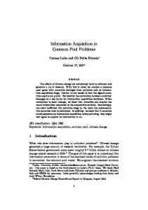
8
positive and negative) so that their Foreign Biasit remains at its initial 2001 level. So for large positive moves in ForeignBiasit this amounts to reducing the eventual increase in the country j holdings of country i, but for large negative moves in ForeignBiasit it amounts to increasing the holdings of that foreign asset. Since this counter-factual includes adjustments that go both in the direction of increasing and decreasing the home bias, it is unclear what would be the overall effect on the counter-factual EHB index. Figure 2: Counter-Factual Home Bias
0.8
Actual Home Bias Counterfactual Home Bias
Home Bias Index
0.75
0.7
0.65
0.6
0.55 2000
2002
2004
2006
2008
2010
2012
2014
Year
The resulting counter-factual EHB index (again averaged over all countries) is plotted in Figure 2. The figure shows that the bulk of the reduction in the home bias has come about as the result of just a handful of big movers in foreign holdings, and not as a broad-based increase in foreign assets. In particular, 83% of the decline in the home bias between 2001 and 2013 is due to the 5% biggest movers in foreign holdings. In particular, if we adjust the holdings of the 5% of biggest movers, so that they do not change their ForeignBiasit index, then the home bias would have decreased by just 0.03 points on average between 2001-2013, but in fact it has decreased by 0.16 points. Thus, we see that relying on the EHB index by itself is hiding some interesting heterogeneity in the trends of specific foreign investments. The fall in the home bias has happened due to the rapid increase in holdings of a few foreign assets in each portfolio, and not because of a general increase in all foreign assets. Even more curiously, there is strong cross-sectional correlation in the identity of the 9
foreign holdings that experience the largest changes across different countries’ portfolios. Simply put, investors across the world seem to increase their holdings of the same handful of OECD countries. To show this, I compute the set of 5% top movers in the foreign holdings in each country’s portfolio, and then construct a histogram to visualize this distribution of destination countries for foreign investment. The result is plotted in Figure 3 below, and show that the increase in investment underlying the drop in the home bias has been disproportionately directed to just a few OECD countries, with the US, UK, France and Germany being one of the most popular destinations. Figure 3: Distribution of the TOP 5 foreign holdings
25
20
15
10
0
Australia Austria Belgium Brazil Bulgaria Canada Czech Republic Denmark Finland France Germany Greece Hungary Ireland Italy Japan Netherlands New Zealand Norway Romania Serbia Spain Sweden Switzerland Tunisia Ukraine United Kingdom United States
5
Overall, the trend downward is clearly an important, robust feature of the data, that goes beyond the opening up of emerging markets and lifting of capital restrictions. However, the underlying increase in foreign investment has not been spread around the world, but has been heavily concentrated in a handful of OECD markets. Understanding these facts can help discipline models of the home bias, and help us better understand the puzzle as a whole.
3
The Model Framework
In this section I turn towards a model that can explain not only the high overall level of the home bias, but also its decline and the fact that the underlying increase in foreign investment 10
has been primarily directed to just a handful of developed markets. I will in particular consider working with a model of information frictions, where the home bias arises due to agents finding it optimal to be better informed about home as opposed to foreign information. I am motivated to work with information models due to abundant evidence that information frictions are important empirical determinants of the home bias (see Ahearne et al. (2004), Amadi (2004), Massa and Simonov (2006)) and the fact that the downward trend in the home bias really started only in the mid-1990s, at the same time as the IT boom which is believed to have greatly driven down the cost of information. The existing information-based models of the home bias have traditionally aimed to understand the average level of the home bias, and are thus static and focus on steady state analysis, and do not speak directly to the evolution of the home bias over time. Nevertheless, at first look it seems like the basic mechanism goes against the observed negative relationship between the home bias and information. A key insight of the previous literature is that information exhibits increasing returns, which leads to full specialization in learning (e.g. Van Nieuwerburgh and Veldkamp (2009)). Thus, agents optimally choose to focus all of their costly information acquisition on domestic information. This is very helpful in generating a high overall level of home bias, because optimal learning endogenously leads to information asymmetry and portfolio concentration. However, at the same time, increased availability of information will tend to increase information asymmetry and thus home bias, and not decrease it. In this section, I extend the model of Van Nieuwerburgh and Veldkamp (2009) to a dynamic setting and show that in this case information acquisition does not display increasing returns globally. It rather exhibits increasing returns when information is scarce, but once information is sufficiently abundant, it has decreasing returns. As a result, a dynamic model of endogenous information acquisition can rationalize both the high level of the home bias, and its trend downwards. The model can also be viewed as a dynamic Noisy Rational Expectations model (NRE), in the spirit of Bacchetta and van Wincoop (2006) and Watanabe (2008), but one where the private signal precisions and information sets are endogenous. There are N countries populated with a continuum of overlapping generations of agents that live for two periods each. In the first period, agents make information and portfolio choice decisions, and in the second they consume their resulting wealth and exit. In each country, there is a Lucas tree with a stochastic dividend. A portion 1 − δ of each tree is traded on international financial markets, and the other δ portion is a non-tradable endowment of the domestic agents. Agents can also trade a riskless bond internationally at a fixed interest rate R, and thus their portfolios are formed by shares in the N different Lucas trees (i.e. risky assets) and holdings of the riskless bond. Each new generation of agents is born with some 11
initial wealth W0 , hence a Young agent in country j at time t faces the budget constraint W0 =
X
pkt xjkt + bjt ,
k
where xjkt is the amount of the risky security of the k-th country he buys, pkt is the equilibrium price of that asset and bjt is the amount invested in the riskless bond. Next period, the agents are in the Old phase of their lives and sell all their assets at the prevailing market prices to the new crop of Young agents, and face the budget constraint cj,t+1 = δdj,t+1 +
X
xjkt (pk,t+1 + (1 − δ)dk,t+1 ) + bkt R
k
where dj,t+1 is the stochastic fruit of the Lucas tree in country j at time t + 1. Thus, δdj,t+1 is the non-tradable endowment of the agents, (1 − δ)dj,t+1 is the dividend of a share of the P risky asset of country j, and k xjkt (pk,t+1 + (1 − δ)dk,t+1 ) + bkt R is the portfolio return. The Lucas tree fruit is the sum of a persistent and a transitory component, dj,t = aj,t + εdjt , where ajt is the persistent economic fundamental associated with country j, and εdjt ∼ N (0, σd2 ) is an iid noise term. I assume that the persistent component of the fundamentals (i.e. country factors) follow symmetric AR(1) processes, aj,t+1 = µj (1 − ρj ) + ρj aj,t + εaj,t+1 with iid Gaussian innovations εajt ∼ N (0, σa2 ). For simplicity, I abstract from comovement across countries, but the framework can easily be extended to accommodate it.
3.1
Information Structure
Agents do not observe the value of the persistent economic fundamental ajt , and have two types of sources of information about it – public and private. First, they have access to private noisy signals about both today’s fundamentals, and any of its innovations up to T < ∞ periods in the future. In particular, for each destination country k, agent i at time t observes the vector of unbiased signals5
5
With a slight abuse of notation, I am suppressing the index of the home country of agent i to save on clutter
where the idiosyncratic error terms εηl kt are iid, mean-zero Gaussian variables. Thus, this is a Hellwig type of dispersed information framework (i.e. beliefs across agents are not perfectly correlated, but there is no systematic error) and multiple countries. Moreover, agents receive private information not only about the value of the fundamental today, but also about future innovations to the fundamental.6 The key to the model is that the precision of the private signals is not fixed exogenously, but is chosen optimally by the agents, subject to a constraint on the total amount of information acquired.7 The amount of information, κ, is measured in terms of Shannon mutual information units (Shanon (1948)). This is the standard measure of information flow in information theory and is also widely used by the economics and finance literature on optimal information acquisition (e.g. Sims (2003), Van Nieuwerburgh and Veldkamp (2010)). It is defined as the reduction in uncertainty (as measured by entropy) about the set of unknown variables {at , εt+1 , . . . , εt+T }, where bold symbols represent the corresponding vector of cross-sectional variables( e.g. at = [a1t , . . . , aN t ]0 is the vector of fundamentals of all N countries), that occurs after observing the private signals of the agents and is given by (i)
κ = H({at , εt+1 , . . . , εt+T }|Itp ) − H({at , εt+1 , . . . , εt+T }|It ) where H(X) is the entropy of random variable X and H(X|Y ) is the entropy of X conditional on knowing Y .8 The set Itp (defined below) is the set of public information that we assume (i) (i) the agent acquires for free, and thus are not subject to the entropy cost, and It = {I˜tp ∪ η t } is the private information set of agent i, which combines the public information with her (i) vector of private signals about the different countries η t = [η1t , . . . , ηN t ]0 . Thus, κ measures the amount of information about the unknown country fundamentals that is contained in the private signals, over and above the free “public” information. 6
This is similar in spirit to the setup in Bacchetta and van Wincoop (2006), but with multiple countries. The idea is that the agents are sophisticated, and can produce information about the unknown fundamentals and their future innovations, but doing so is costly in terms of time, money and mental effort, resulting in a finite information capacity. Instead of fixing the information capacity, I could have equivalently assumed that the agents face a convex cost of information, C(κ) – this would lead to the same results but will complicate the exposition. 8 Entropy is defined as H(X) = −E(ln(f (x))), where f (x) is the probability density function of X. 7
13
Given the prior assumption that all factors are uncorrelated across countries, we can express the total information acquired κ as the sum of the information acquired about each country individually κ = κ1 + · · · + κN Where the the information of each individual signal is similarly defined as the information about a given country’s fundamentals over and above the costless public information: (i)
κk = H({akt , εak,t+1 , . . . , εak,t+T }|Itp ) − H({akt , εak,t+1 , . . . , εak,t+T }|{Itp , ηkt }) In order to keep things tractable, I assume that the public information set consists of the current value of dividends and equilibrium prices: Itp = {dt , pt } Among other things, this means that the agent will not use past dividends and/or asset prices to update his beliefs, even though those are also informative signals. This assumption is made mainly for tractability purposes in the hopes of achieving some analytical results. However, it could be relaxed in numerical exercises without loss of any particular economic insight. One interpretation of this setup is that extracting information from the publicly available variables is not “free” either, since it requires both effort and resources, and as a result the agent only pays attention to the most current (and accurate) public variables.9 After observing all available signals, the agents use Bayesian updating with the correct priors to form their posterior beliefs. Contrary to the standard approach in the literature, I assume the agents have identical priors over both the home and foreign factors, and hence there is no exogenously imposed information advantage. The goal is to study the properties and extent of information asymmetry that can arise purely as a result of endogenous forces, but introducing some prior informational advantages would not change the analysis qualitatively.10 Lastly, I assume that the agents’ have mean-variance utility over their end-of-life consumption, γ (i) (i) (i) (i) U (i) = E(ct+1 |It ) − Var(ct+1 |It ) 2 where γ is the absolute risk aversion coefficient (common across all agents). This is the standard utility function used in the literature on endogenous information choice and portfolio 9
The most expansive public information set we can consider is the one consisting of the whole history of dividends and prices. In that case, equilibrium prices will become functions of the conditional expectations coming out of the Kalman filter, but would not change other things qualitatively. 10 Note that newly born generations do not inherit the private information of older generations, hence there is no long-lived private information and no need to keep track of the dynamics of the distribution of beliefs.
14
choice due to its analytical tractability (Van Nieuwerburgh and Veldkamp (2009, 2010), Mondria (2010)). In essence, this is an en exponential (CARA) utility function with an added desire for early resolution of uncertainty.11 The results also hold under CRRA, but the mean-variance function is more convenient for showing the results analytically.
4
Analytical Model – T = 0
In this section I consider the version of the model where agents only receive private information about today’s fundamentals akt and thus T = 0. This simplifies the beliefs updating step and the eventual information choice of the agent, who needs to solve only for his attention allocation across countries, but not also about how to allocate information between news about the future and information about today. The end result is an analytically tractable model. In a later section I relax this assumption, and numerically examine the new forces introduced once we allow for T > 0. The model is solved in two steps. First, I derive the optimal portfolio choices and resulting asset market equilibrium given a fixed information choice. And then second, using the knowledge of the portfolio choices given an information structure, I find the optimal information acquisition choice of each agent.
4.1
Portfolio Choice and Asset Market Equilibrium
Since dividends are Gaussian I conjecture and later verify that the equilibrium prices pkt are linear in the state variables, and hence are Gaussian as well. Thus, the posterior beliefs of the agents follow a Normal distribution, which leads to the familiar mean-variance optimal portfolio holdings:
(i)
(i) xjjt
=
E(pj,t+1 + (1 − δ)dj,t+1 |Ij ) − pjt R (i)
γ Var(pj,t+1 + (1 − δ)dj,t+1 |Ij )
(i)
−
Cov(δdj,t+1 , pj,t+1 + (1 − δ)dj,t+1 |Ij ) (i)
Var(pj,t+1 + (1 − δ)dj,t+1 |Ij ) (i)
(i) xjkt
=
E(pk,t+1 + (1 − δ)dk,t+1 |Ij ) − pkt R (i)
γ Var(pk,t+1 + (1 − δ)dk,t+1 |Ij )
(i)
where xjkt is the amount of the risky asset of country k, that the i-th agent in the j-th country buys. There are two motives for buying the risky assets – a speculative one and a hedging one. For speculative purposes, agents like to buy assets that offer high expected 11
See Van Nieuwerburgh and Veldkamp (2010) for more details.
15
excess returns and not too much variance. In addition, the home asset (xjjt ) is also useful for hedging the risk coming from non-tradable income – this is captured by the covariance (second) term in the first equation. Two forces could potentially affect the agent’s desire to alter her portfolio holdings from being split equally between all available assets. One is the additional hedging motive to trade the home asset, and the other is any potential information (i) (i) asymmetry, Var(pj,t+1 + (1 − δ)dj,t+1 |Ij ) 6= Var(pk,t+1 + (1 − δ)dk,t+1 |Ij ) for j 6= k, which would alter the speculative portion of the portfolios. In addition to the informed traders, each risky asset is also traded by a measure of “noise” traders, who trade for reasons exogenous to the model. The net noise trader supply of asset k is zkt ∼ iidN (0, σz2 ). Market clearing requires that the sum of the informed agents trades and the noise traders equals the asset supply, z¯k , and thus for each asset we have the market clearing condition Z 1 X (i) z¯k + zkt = xjkt di N j
(2)
I look for a linear stationary equilibrium where equilibrium prices are time-invariant, linear functions of the state variables. Because of the linear-Gaussian information structure, conditional expectation, and hence also portfolio holdings, are linear in the information sets of the agents. Substituting this in the market clearing condition (2) results in equilibrium prices that are linear in the aggregate information set: ItAgg = {dt , at , εt+1 , . . . , εt+T , zt } This is the information set that would result if we were to aggregate the information of all market participants. It includes the realizations of the latent fundamentals ak,t because the noise in the private signals of the agents is iid, and hence aggregating over them perfectly reveals the underlying fundamentals. Moreover, notice that if an agent knew the value of the akt terms, then he is also able to uncover the measure of noise traders zkt from the equilibrium price. Thus, the aggregate information set contains both the future fundamentals, and the current measure of noise traders, both of which are unknown to any single investor. Furthermore, since the fundamentals and the noise traders are independent across countries, each equilibrium price is a function of only domestic variables and takes the form, ¯ k + λak akt + λdk dkt + λzk zkt , pkt = λ ¯ k , λak , λdk , λzk are determined by the market clearing conditions. The where the coefficients λ
¯ + Λ k ρa a =λ ˆk,t where for notation convenience I define Λk as the loading of the asset return on the unknown (i) ak,t+1 , and conditional expectations as hatted variables, so that xˆt = E(xt |It ). Similarly, the conditional variance is (i)
2 where hatted σ ˆkt = Var(akt |It ). Notice that agents are faced with two types of uncertainty – learnable and unlearnable (i.e. some unknown variables are outside of today’s scope of learning). The agents can use their costly information acquisition to reduce uncertainty about today’s fundamentals akt , however, the asset returns pk,t+1 + (1 − δ)dkt − Rpkt are also affected by several variables – namely the future innovations εak,t+1 , εdk,t+1 , zk,t+1 – that are outside of the learning scope of today’s agents. This is worth nothing here, because it will have important implications about the returns to information later. A portion of the unlearnable uncertainty depends on the equilibrium coefficients of the future asset price, and will thus be determined by endogenous equilibrium forces. On the one hand, part of the unlearnable uncertainty comes from the fact that the future asset price pk,t+1 has a loading of λak on the future fundamental innovation εak,t+1 . As we will see below, the size of this coefficient depends on the information choice of the future generation – if they choose to not acquire any information about the fundamentals, then λak = 0, and there will be no uncertainty coming from this term. While the more information they do acquire, the large will λak be. On the other hand, there is also unlearnable uncertainty coming from two other sources d – εk,t+1 and zk,t+1 . These sources of uncertainty are “unlearnable” by assumption since we have assumed that agents can receive signals only about the persistent fundamentals, but not about any of the noise terms. However, it is worth nothing that this assumption is made primarily for tractability reasons. It is interesting to consider what happens if we were to allow the agents to receive signals about all contemporaneous unknown variables. Then the weight on the future innovations of those variables will again be determined by the
17
information choice of the future generation, while they’ll be outside of the learning scope of today’s agents. In other words, the basic insights of the current model would hold as long as we have a dynamic model where the scope of learning grows over time, so that with the passage of time more learning opportunities open up. As long as the scope of learning in the future is bigger than the scope of learning today, then there will be some unlearnable uncertainty facing agents because of future information acquisition getting incorporated in the future asset prices. Thus, more generally, today’s agents face some unlearnable uncertainty in the future valuation of the asset, pk,t+1 , because the information available to them today does not fully span the market beliefs tomorrow. This is a reflection of the fact that information sets are recursive, and grow over time: Agg Agg ItAgg ⊂ It+1 and It+1 \ItAgg 6= ∅ Agg Agg Since, ItAgg is coarser than It+1 , the future aggregate information set It+1 contains uncertainty that is unlearnable for agents at time t. This is a result of the recursive structure of the dynamic model, which leaves future agents one-step ahead of today’s agents. But more generally, the key assumption is that the information available today does not fully span future market beliefs and as a result, agents always face some measure of unlearnable valuation risk. Here, I model this by assuming that there is a finite future horizon at which agents can learn, but it could also be done in other ways. The conditional expectation and variance of the unknown fundamentals akt follow the standard formulas for updating Gaussian variables with Gaussian signals. The agents have (i) three sources of signals, the idiosyncratic signals ηkt , the current level of dividends dkt , and the equilibrium asset prices pkt , which they combine with their priors to compute,
Plugging everything back in the market clearing condition (2) gives us the solution for the coefficients of the equilibrium prices. I will focus on a symmetric equilibrium where all agents in each country make the same information choices, so we can dispense with the i
18
subscripts and focus only on the country subscripts j. The details of the derivations are given in the Appendix, and here I will just highlight the structure of the two most important coefficients – the ones on the unknown fundamental and noise term: σ ¯k2 q¯k φ¯k q¯k (1 + 2 2 ) R γ σz 2 φ¯k q¯k γσ ¯ = − k (1 + 2 2 ) R γ σz
λak =
(4)
λzk
(5)
where I define σ ¯k2 as the average market participant’s posterior variance of the return of the k-th asset, which is given by σ ¯k2 =
1 1 X (i) N j Var(pk,t+1 + (1 − δ)dk,t+1 |Ijt )
!−1
where we sum over the countries j and q¯k is a weighted average of the precision of the private signals of all market participants, q¯k =
2 X 1 Λk ρ2k σ ˆjkt 1 2 (i) N Var(pk,t+1 + (1 − δ)dk,t+1 |Ijt ) σj,ηk j
and φ¯k is the fraction of learnable uncertainty in total uncertainty, averaged across all market participants: φ¯k =
2 X 1 Λk ρ2k σ ˆjkt (i) N Var(pk,t+1 + (1 − δ)dk,t+1 |Ijt ) j
To gain more intuition about the price coefficients, note that we can re-write λak as λak
ρa Λk = R
2 σ ˆjt 1 X σ ¯k2 1− (i) σa2 N j Var(pk,t+1 + (1 − δ)dk,t+1 |Ijt ) 1−ρ 2 a
!
which shows that it is a decreasing function of the weighted average of the ratio of the 2 σ ˆjt posterior variance of akt (across agents in different countries) and its prior variance – σ2 . a
1−ρ2a
Thus, the more information the market as a whole has about akt , the higher is λak . In the extreme of no information about akt , λak = 0, and in the other extreme where everyone knows akt perfectly λak = ρaRΛk which is the discounted value of the cash flows due to akt . Intuitively, as market participants acquire more information about some of the unknown fundamental terms, they trade more aggressively on that information and thus it gets reflected more
19
strongly in the asset price. 12 Lastly, the price coefficients on the noise traders term is also quite intuitive. First, it’s negative, since more noise traders increase the required risk-premium for the informed traders to absorb the increased supply. Second, its absolute value is increasing in risk aversion γ and the average market posterior variance of asset returns. Since holding the risky assets exposes agents to variation in noise trader demand, they require a compensation, and that compensation is increasing in the total amount of uncertainty faced and the price of that uncertainty – the average market posterior variance of asset returns and the investor’s risk aversion.
4.2
Information Choice
Information choice happens before the asset markets open up and before the current period dividends are realized. In the information choice step, the agent chooses the precision of his private signals to maximize his expected utility, taking as given his optimal portfolio choice as a function of his information choice. Since there is one-to-one mapping between the precision of the signals and the total amount of information (in entropy units) contained in each signal, 2 κk = ln(Var(akt ) − ln(ˆ σkt )
we can express the choice of the agent as a choice over the amount of information allocated to learning about each country’s fundamentals κk . Thus, the information choice problem of the agent becomes max E(Uj (x∗t (ηt )))
κ1 ,...,κN
s.t. X
κk ≤ K
k
κk ≥ 0 thus choosing the informativeness of his signals to maximizes his expected utility integrating over the unknown realizations of his private signals, taking as given the optimal portfolio choice x∗t as a function of his information choice. The first constraint says that the agent can use up to no more than K bits of total information (this is the information capacity 12
As is known, the equilibrium in the dynamic NRE models is not necessarily unique. In fact, there can be up to 2N different equilibria – see Watanabe (2008). For most of the analytical result, the equilibrium selection does not matter. For numerical results, as is standard I will focus on the “low volatility” equilibrium, which is the unique stable one.
20
constraint), and the non-negativity constraint is a “no forgetting constraint”, meaning that the agent cannot choose to obtain “negative” information about one of the assets, which will be equivalent to “loosing” information from one of its priors. First, I confirm that the information choice is indeed time-invariant, which would validate our earlier assumption that the equilibrium prices are time-invariant functions of the state variables. The result is formalized in the proposition below. Proposition 1. The optimal allocation of information is time-invariant, i.e. κkt = κk for all k and t. Proof. Intuition is sketched out in the text, and details are in the Appendix. This tells us that at any time period t, the currently young generation (of any country – note that country subscripts are suppressed to reduce clutter) allocates its finite information capacity in the same way that next period’s generation would do, and last period’s did as well. Thus, the posterior variance of the average market participant is time-invariant. Going back to the formulas for the equilibrium price coefficients given above, we see that this guarantees that they do not change over time either, and hence we have a stationary equilibrium. To gain intuition about the result, it’s useful to derive the ex-ante expected utility that enters the information choice. E(U (x∗t )|at ) = W0 R + δρa ajt +
−
(i) 1 X Var(E(exk,t+1 |It )) + (E(exk,t+1 ))2 (i) 2γ k Var(exk,t+1 |It )
where exk,t+1 = pk,t+1 + dk,t+1 − Rpkt is the excess return of the k-th asset. Information enters the agent’s expected utility in two ways. First, it alters his optimal speculative portfolio, which effect is given by the summation in the third term, and it alters his optimal hedging portfolio, which operates through the last term. From a return maximization perspective, information about all k assets is symmetric, but only home information helps in forming the hedging portfolio, and hence the last term is not a summation. We can then derivate in respect to κk to see what is the marginal benefit of an extra unit of information about the k-th asset. To make the notation less burdensome let γδ 2 ((λjd + (1 − δ))2 σd2 + λ2zj σz2 ) B = δE(exj,t+1 |a ) + , 2Λk t
The expression shows three main things – agents like to learn about assets that 1) have high ex-ante expected excess returns, 2) have ex-ante volatile expected excess returns, and 3) prefer learning about the home asset (B > 0). Understanding these effects starts with the fact that information is non-rival, in the sense that a unit of information can be equally applied to optimizing one’s returns and to forming a better hedging portfolio. The third effect is perhaps the easiest one to understand – the home asset does not offer only potentially high excess returns, but also the benefit of hedging the non-tradable labor income of the agents. As a result, ceteris paribus, home information is the most valuable, because it can help in both forming a better speculative portfolio, and a better hedging portfolio. The fact that agents like to learn about assets with high ex-ante expected excess returns is also quite straightforward. Those are attractive assets on average, and hence are likely to represent a bigger portion of the total portfolio of the agents. Since information is non-rival, it is better to apply a unit of information to a big portfolio holding, rather than to a small one, and hence agents want to maximize learning about assets they expect to be a big part of their portfolios. On the other hand, agents also like to learn about assets with volatile ex-ante expected excess returns. Such assets are more likely to present profitable trading opportunities once the private information is realized, since they can either feature an abnormally high or low expected return, and thus form a relatively big part of the agent’s portfolio. The other reason is that volatile excess returns indicate that the market does not posses good information about the underlying fundamentals and hence mis-prices them. The private information of the agent can help identify and profit from such mis-pricing mistakes. To see this more clearly, note that the fundamentals related terms in the realized excess returns are exk,t+1 =
1 σ ¯k2 φ¯k (
− ρ2 1 + 2 )at + Λk εak,t+1 + . . . 2 σa σd
(7)
Clearly, when the future innovation of the fundamentals is high, the realized excess return is also high since the future innovation is pure news to the market and is not incorporated in the current equilibrium price. The return is also increasing in akt since today’s fundamental is persistent and will also affect the future level of dividends. However, the extent to which the excess return responds to movements in akt depends on how much the market knows 22
about akt . If the market has perfect information then σ ¯k2 → 0 and the excess returns does not respond to movements in akt at all. This is because when that variable is known to all market participants, then its value is already fully incorporated in today’s price and would not affect the excess return. Hence, high volatility indicates that the market leaves some of the variation in the current fundamentals mis-priced, and this is the type of variation private information can help agents exploit. In particular, the way the expected excess return responds to movements in akt is 2 Et (exk,t+1 ) = (¯ σk2 φ¯k − Λk ρˆ σjk )
1 − ρ2 akt + . . . , σa2
2 ˆjk > 0, the which shows that when an agent is better informed than the market, σ ¯k2 φ¯k − Λk σ agent’s expectations correctly time the market. They go up when the actual excess return is indeed likely to be high and vice versa. Thus, superior information helps the agent engage in profitably exploiting the pricing mistakes of the average market participant. To show that the information acquisition strategy does not vary over time, we need to show that the ex-ante expected excess returns and variances are not time-varying. The ex-ante excess return is given by
Basically, the average excess return on risky assets reflects the compensation agents require for holding the full supply of the risky asset. The net supply of the asset, the expression in the brackets above, has two components. The first one is the exogenous fixed supply and the second, is any extra net supply coming from the hedging activity of the agents in country k. In effect, this increases the total supply of the asset that needs to be soaked up by the speculative portfolios. Since supply is exogenously fixed over time, if the information 2 strategy itself does not vary (i.e. σ ˆkk is time invariant) then ex-ante expected excess returns do not vary over time either. The details of the proof amount to showing that since the ex-ante excess return is given by the same function each period, agents have no incentives to vary information acquisition. On the other hand, the ex-ante variance can be expressed as Var(E(exk,t+1 |It )) = Var(Λk ρakt − Rpkt ) − Λ2k ρ2 σ ˆk2 which shows again that if information choice does not vary over time, then this variance term does not vary either. And we can again show that there is no incentive to change information
23
choice, and thus there is an equilibrium where information acquisition is time-invariant. Lastly, note that if we combine all of these results, we arrive at the conclusion that in the symmetric equilibrium (where all asset returns and variances are ex-ante symmetric) we have home bias in information acquisition. This is essentially due to the dual nature of the home asset, as both an investment and a hedging vehicle. The result is summarized by the proposition below. Proposition 2. If δ > 0 agents in country j optimally chooses κj > κk for all k 6= j, i.e. they choose to acquire more information about the home fundamentals. Proof. Follows from symmetry, the fact that information is non-rival, and the positive correlation between the domestic risky asset and non-tradable domestic income. Details are in the Appendix.
4.3
Information Specialization
Increasing returns to information are the principal feature of the standard, static models of information and portfolio choice. This incentivizes agents to fully specialize in learning, and thus only acquire domestic information, which is at the heart of the models’ ability to generate home bias. In this section, I show that the desire to specialize in the dynamic model is more nuanced, explain the differences and why they arise. To understand when and why increasing returns to information obtain, it is useful to compute the derivative of the marginal benefit of extra information. Full details are given in the appendix, but it can be shown that it is proportional to ∂M Bk ∝ ∂κk
Thus, the marginal benefit of information is increasing whenever the amount of learnable uncertainty left in a given asset’s return is greater than the amount of unlearnable uncertainty. The key to understanding the increasing returns is that information is non-rival, and hence one unit of information could be as easily applied to a $1 bet as to a $100 bet. However, a unit of useful information leads to bigger trading profits when applied to a bigger portfolio holding. This generates a feedback effect between information and portfolio choice. In particular, as κk increases, the posterior variance of asset k decreases, and hence the agent expects to hold more of that asset (xk goes up). As expected holdings increase, however, the expected benefit of an extra units of information about the k-th asset increases as well – the more informed you are about an asset, the more of that asset you tend to hold, and thus the more useful the 24
next unit of information. This feedback loop is the only effect in the benchmark static model, and results in global increasing returns to information. In the dynamic model, however, there is also an additional effect – increasing asset holdings exposes the agent to progressively larger amounts of unlearnable valuation risk. Recall that the return of asset k does not depend only on learnable uncertainty about the value of akt , but also on the future innovations to fundamentals, dividends and noise trading, which all affect the asset return through their effect on the future price pkt . This moderates the incentive to increase portfolio holdings in response to an increase in κk , and weakens the feedback loop described above. When agents have not acquired much information about asset k, the posterior variance of the current fundamental is relatively high, and as a result learnable uncertainty is the majority of total uncertainty, and hence the first effect dominates and information displays increasing returns. However, when information is abundant, the majority of remaining uncertainty is unlearnable, and in this case the second effect dominates and information displays decreasing returns. This is formalized in the proposition below. Proposition 3. Increasing returns to information exist when the asset in question has more learnable uncertainty remaining, than unlearnable uncertainty, i.e.: ∂M Bk ∝ ∂κk
In particular, this means those are assets that: 1. The agent has not learned much about – high σ ˆk2 2. Feature less unlearnable uncertainty – low Λ2k σa2 + (λdk + (1 − δ))2 σd2 + λ2zk σz2 The proposition has two main implications. First, as an agent learns more and more about a particular asset, the returns to information generally decrease. Even if an asset exhibits increasing returns when the agent has acquired no information, eventually, as the agent acquires more information that asset will start to exhibit decreasing returns. This is because only a portion of the total uncertainty about an asset’s payoffs is learnable. Hence, as the amount of information that has already been acquired increases, the next unit of information reduces an ever smaller portion of the remaining uncertainty, which weakens the feedback between portfolio and information choice. Thus, agents face increasing returns to information when information is relatively scarce, and decreasing returns otherwise. The second interesting result is that whether information features increasing or decreasing returns also depends on the structure of the equilibrium price pkt , which determines the size of the unlearnable uncertainty. In particular, assets for which the price is more 25
responsive to innovations to fundamentals and dividends or noise trader shocks, are more likely to feature decreasing returns to information. This will have important implications as to whether information is a strategic substitute or a strategic complement, as discussed in more detail in Section 4.5.
4.4
Information Capacity and Optimal Information Acquisition
Next I turn to the optimal information choice as a function of the information capacity of the agent K. The main result is that agents tend to focus information acquisition one asset at a time, and expand the portfolio of assets they learn about as their information capacity increases. The particulars are formalized in the proposition below. ¯0 < K ¯1 < · · · < K ¯ N −1 } such that if Proposition 4. There exist positive constants {K ¯ 0 – agents specialize fully in learning about the domestic asset: κj > 0, κk = 0 • K≤K for all other k ¯ L−1 , K ¯ L ] – agents learn about home and L > 0 foreign assets: κj > 0, κk0 > 0 • K ∈ (K for L different k 0 6= j, and κk = 0 for all other k ¯ N −1 – agents learn about all assets: κk > 0 for all k. • K>K Moreover, all foreign assets that the agent chooses to learn about receive the same amount of information acquisition. Thus, for any two k, k 0 where κk > 0, κk0 > 0 we have κk = κk0 Proof. Sketched in the text, details in the Appendix. The general intuition for the result follows from the conditions under which information displays increasing returns. As we saw in Proposition 3, increasing returns obtain when the agent has not learned much about a particular asset. Moreover, from Proposition 2 we know that the most preferred asset is the home asset. As a result, when information information is ¯ 0 , the agent finds it optimal to fully specialize in learning only relatively scarce, i.e. K ≤ K about the home fundamental. This is the best use of the scarce information. As information capacity increases, however, the agent moves into the part of the parameter space where home information starts exhibiting decreasing returns, and thus eventually finds it optimal to start acquiring information about foreign assets as well. However, this information diversification does not happen smoothly across all assets. Rather, at first ¯ 0, K ¯ 1 ], the agent only acquires information about one foreign asset, then as when K ∈ (K information capacity increases further, he adds a second foreign asset to his learning portfolio and so on. Eventually, when information is sufficiently abundant, he would be learning about 26
all assets. Thus, as information capacity increases, it percolates in a step-wise fashion through the whole menu of available assets. The particular structure of the problem implies that the information asymmetry of home vs foreign information is non-monotonic in information capacity. When information is relatively scarce, the agent fully specializes in home information and does not acquire any foreign information. In that part of the state space, as information capacity rises, the asymmetry is in fact rising, because the agent invests more and more resources into home information, but does not acquire any foreign information. But once the ability of the agent ¯ 0 , the agent starts acquiring to acquire information increases sufficiently, so that K > K foreign information as well. As a result, as the information capacity increases, the agent is gradually diversifying his learning into foreign information, and his overall information asymmetry decreases as well. Lastly, it is interesting to note that, in the symmetric equilibrium case we are currently analyzing, the agent splits the foreign assets into two groups – those he chooses to learn about and those he chooses not to. If at any point the agent chooses to learn about more than one foreign asset, then those assets will all receive the same amount of information acquisition. The intuition is that it is only beneficial to learn about more than one foreign asset when information capacity is sufficiently abundant so that the agent has fully exhausted the increasing returns of the first foreign asset. But once he decides to add a second foreign asset to his learning portfolio, it is again best to fully exhaust the gains to specialization in that asset immediately as well. And thus, whenever the agent is learning about two foreign assets he is in fact on an interior solution for information allocation, and since all foreign assets are symmetric, this results in κk0 = κk for any two foreign assets k 0 and k that the agent decides to learn about. So then even though home vs foreign information asymmetry is falling monotonically with information costs, the foreign assets are not treated as a homogeneous group that all rise all together. In fact, the agent specializes in a subset of the foreign assets, and completely ignores the others. As a result, the concentration of the foreign holdings of the agent are in fact also at first increasing, and then decreasing as information costs fall. That is because initially the agent specializes learning in just one or two foreign assets, and only eventually gets around to learning about all foreign assets.
27
4.5
Strategic Substitutability and Complementarity in Information Choice
In the previous section we considered what happens to information choice as the information capacity of a single agent changes. Here we turn to the question of how the aggregate information capacity affects an individual’s information choice. The bottom line result is that the model features forces of both strategic substitutability and strategic complementarity, and which one dominates depends on parameters. In the standard static model information is a pure strategic substitute, and many of the same forces are active in the dynamic model as well. Primarily, when the precision of private information about asset k increases, naturally the different agents’ posterior variances of the 2 unknown fundamental, σ ˆjk , decrease. In turn, this lowers the average market participant’s posterior variance of the return ( i.e. σ ¯k2 ), which lowers both the ex-ante expected excess return and the ex-ante volatility, which in turn decreases the marginal benefit of learning about that asset (see eq. (6)). Thus, through this channel, an increase in the market’s information about a particular asset will lower the incentive for learning about that asset. Moreover, in the dynamic model there is also another force for strategic substitutability, which works through the endogenous part of the unlearnable uncertainty. As the precision of private information increases, the agents tend to act on it more aggressively and as a result the value of the price coefficient on the fundamental λak increases (see eq. (5)). In turn, this raises Λk , the elasticity of the asset return to εak,t+1 . As the returns become more sensitive to movements in future innovations the unlearnable uncertainty increases, and this puts downward pressure on the incentives to specialize in information about that particular asset (i.e. agents are faced with decreasing returns to information earlier). The more informed is the average market participant, the more exposed you are to unlearnable risk. However, in addition to these two forces for strategic substitutability, the dynamic model also features two channels for strategic complementarity in information choice. An 2 increase in the precision of private information does not only lower σ ˆjk across the board, but also increases λak and thus Λk . But note that the conditional variance of the asset return is 2 2 Λ2k ρ2a σ ˆkt + Λ2k σa2 + (λdk + (1 − δ))2 σd2 + λ2zk σzk
which is increasing in Λk . Hence, holding a given agent’s information fixed, if everyone else becomes better informed then Λk increases, σ ˆk2 stays constant, and thus the posterior variance of the excess return increases. Essentially, since now the rest of the market is better informed and thus is acting more aggressively on their private information, this makes expected excess returns more responsive to fundamental news and thus more volatile. Increased information 28
increases the role of the asset pricing factor that is due to today’s information about akt . On the one hand, this force exerts an upwards pressure on σ ¯k2 and thus on ex-ante excess returns and variances. On the other, the increase in Λk also has an additional, direct effect pushing up both of these ex-ante moments. In terms of the expected excess return, an increase in Λk increases the hedging-driven component of the ex-ante expected return. In terms of the ex-ante variance, an increase in Λk unsurprisingly increases the ex-ante variance of realized excess returns term – Var(Λk ρakt − Rpkt ). Both of this tend to push higher the marginal benefit of information and thus serve as incentives for strategic coordination in information choice. In addition, an increase in the aggregate market information can also increase learnable uncertainty. As Λk goes up, this increases the share of the total asset return variance that is attributable to fluctuations in today’s fundamental, which the agents can learn about. Essentially, this increases the scope of learning for today’s agents. When there are better informed traders the future asset price pkt is more highly dependent on the value of fundamentals. Today’s agents cannot learn directly about the future fundamental innovation, but since akt is persistent information about today’s value is still useful in forecasting the future price. This channel is due to the “beauty contest” nature of dynamic asset markets. Informed investors have incentives to forecast not only future dividends, but also the future market price, which depends on future market beliefs. As a result, agents try to forecast those future market beliefs and trade accordingly, and this affects their information choice. If markets are relatively well informed about a particular asset then the average market belief is more closely aligned with fundamental fluctuations, which increases the incentives for an individual agent to learn about that asset’s fundamentals. Intuitively, investors do not want to invest scarce information acquisition in finding an obscure under-valued asset if the market never wakes up to its under-valuation. Investors want to identify assets that are both i) mispriced by the market currently and ii) the market is likely to correct in the future. At the end of the day, while all of these forces are present in the model, which one dominates depends on parameters. For example, a higher Λk tends to increase both the learnable and unlearnable components of uncertainty. Which effect dominates depends on the persistence of the fundamental ρ, and the relatively size of Var(akt |dt ) and σa2 . I explore these issues in more detail in a later section focused on numerical exercises.
29
4.6
Optimal Portfolios
As a result of the step-wise nature of optimal information acquisition, the optimal portfolio is formed by three types of assets – the home asset, the foreign assets that the agent does learn about, and the foreign assets he does not. This gives rise to a three-fund separation theorem. In particular, the optimal risky asset portfolio is a convex combination of 1) a fund holding 100% domestic assets, ¯ zj , 2) a fund that is perfectly diversified over the foreign assets the agent does learn about and holds nothing else, ¯ zj,learn , and 3) a fund that is perfectly diversified over the foreign assets he does not learn about ¯ zj,no learn . The aggregate portfolio of country j can be expressed as, x ¯j = α¯ zj + β1¯ zj,learn + β2¯ zj,no learn This follows directly from previous results. The agent always finds it optimal to learn the most about the home asset, hence there is asymmetry in home vs foreign information which affects home vs foreign holdings. However, the agent does not treat all foreign assets symmetrically. There is a subset of assets (possibly empty) that the agent allocates positive information acquisition to, and the rest of the assets do not receive any information. The agent treats all foreign assets within each subclass equally, which generates the three-fund theorem above. It is interesting to consider how the portfolio holdings are adjusted when information capacity increases. The first and most obvious effect is the “home bias”, which measures the relative holding of home versus all foreign assets. In a model with no learning and no non-tradable income in equilibrium all agents hold the market portfolio (also known as the CAPM portfolio): x ¯M KT = ¯ z. To illustrate what happens when we introduce non-tradable income δ > 0 and learning, I will use an example with just two symmetric countries, a home and a foreign one. The equilibrium portfolios become oInf o x¯N = z¯h − h
where a subscript h denotes the home country and f denotes the foreign country. Compared to the CAPM portfolio, this one is tilted towards foreign assets due to the hedging motive 30
introduced by non-tradable income. The portfolios exhibit foreign bias, because of the negative hedging demand for the home asset. So the hedging channel by itself is not helping in generating home bias, but is in fact doing the opposite. The information channel that works in the opposite direction by generating information 2 asymmetry, where agents are better informed about the home asset. Letting σek = Λ2k σa2 + (λdk + (1 − δ))2 σd2 + λ2zk σz2 denote the amount of unlearnable uncertainty agents face, then when agents can acquire information, the resulting optimal portfolio of the home agent is:
The information effect comes from the fact that in the (symmetric) equilibrium home agents are better informed about the home asset than the market as a whole and thus 2 ˆh + σeh σ ¯h2 > Λ2h ρ2 σ . The bigger is this difference, the larger is the tilt towards home assets than comes from the information channel. Moreover, notice that increased information about the home asset also tends to lower the negative effect of the hedging demand Thus, the overall level of the home bias depends on the equilibrium information asymmetry. And since this asymmetry is non-monotonic in K, the home bias in portfolios unsurprisingly inherits a similar property. This is illustrated in Figure 4, which plots the Equity Home Bias index (EHB) for an investor in an economy with five countries (N = 5). The home bias is at first increasing in K, but is then decreasing beyond a threshold value for K. Thus, we see that information frictions could potentially generate meaningful home bias in intermediate values of information capacity, but also as information grows its effect is gradually unwound. Figure 4 also hints at another interesting feature of the model – the increased investment in foreign assets that comes with larger K is not spread out equally across all foreign assets. As we know from Proposition 4, an agent learns only about a subset of the available foreign assets, and moreover any assets that he learns about are treated equally. Thus, as K increases enough to incentivize the agent to start acquiring foreign information, at first he only focuses on one of the foreign assets. As information capacity increases further, he finds it optimal to learn about an additional foreign asset and so on and so forth. This can be seen from the kinks in the EHB (blue line) as information costs fall. At first the home bias is falling smoothly, and this is the region in which the agent is learning only
31
Figure 4: Portfolio Bias and Information Capacity Change in Individual Information Cost
Equity Home Bias Index (EHB)
End Info Choice No Information
0
0
5* (Information Capacity)
about the home asset and one foreign asset. Then as information costs fall further, there’s a discrete drop in the home bias, which happens at the point where there agent starts acquiring information about a second foreign asset. As information at first enjoys increasing returns, it is never optimal for the agent to learn just a little bit about the new foreign asset, while still learning a lot about the initial foreign asset he started learning about. Instead, there’s a discrete jump in the amount of information acquired about this second asset. Then the agent keeps investing in acquiring more information about those two foreign assets together as a bundle, until a point at which he finds it optimal to learn about three foreign assets and etc. Therefore, as the home bias falls with the increase in information capacity, the foreign portion of the portfolio is undergoing its own non-monotonic adjustment in concentration. When information is relatively scarce so that the agent only acquires home information, he holds a under-weighted position in a perfectly diversified foreign fund. However, as K increases and he diversifies learning, the concentration of the agent’s foreign holdings increases. At first he specializes in one foreign asset, then in two, three and so on. In the limit, he goes back to a perfectly diversified foreign fund. Thus, in the parameter space where the home bias is falling, the concentration in the foreign portion of portfolios is non-monotonic. This is illustrated by Figure 5, which plots a concentration index for the foreign holdings of the 32
Figure 5: Concentration of Foreign Holdings and Information Capacity
Bias in Foreign Portfolio
Change in Individual Information Cost
0 0
5* (Information Capacity)
agents. As we can see, at first concentration among foreign holdings is increasing, and then it decreases.13 It is also interesting to consider the effect on the non-tradable income. On the one hand, it generates a negative hedging demand, which is best seen in the fact that the EHB index for low values of K is negative in Figure 4. On the other, the fact that the non-tradable income is correlated with the domestic dividends gives the agents an incentive to value home information more than foreign information, and is the reason that agents focus their learning on home information. Thus, it is a big part of the reason that the EHB index is initially strongly increasing with K. Figure 6 illustrates this by comparing the resulting home bias with a model where there is no non-tradable income (δ = 0), but instead agents have a small information advantage over home information. As we can see, in that case we can still generate some home bias, due to the initial desire to specialize, but the incentive to specialize wears off much quicker. As a result, the overall level of the home bias that can be achieved is much smaller, and comes at a lower level of total information acquired.
13
It plots the bias index defined as
1 k N −1 |Foreign
P
Biasik |, where Foreign Biasik =
33
P xik / P z¯k z¯k k6=i xik k6=i
−1
Figure 6: Effect of Non-Tradable Income No Labor Income
Equity Home Bias Index (EHB)
$ / >0$ $ / = 0$
0
0
5* (Information Capacity)
5
General Equilibrium and Numerical Exercises
In this section, I consider the full version of the model where agents can also learn about future innovations to the fundamentals (T > 0). Moreover, while previously we focused on analyzing an individual agent’s optimal actions keeping the rest of the market fixed, here we will also solve for the general equilibrium distribution of information and portfolios. Allowing agents to learn news about the future serves two purposes. First, it not only increases the scope of learning by expanding the learnable portion of uncertainty, but there is also a complementarity between learning about the current fundamentals and about future innovations to the fundamentals. As a result, the marginal benefit of information about akt is increasing in the information acquired about εk,t+l . Both of these forces serve to amplify the amount of information asymmetry, and thus portfolio home bias that can be achieved in equilibrium. Second, it also increases the forces for strategic complementarity in information acquisition across agents. These two effects are best understood by examining the structure of the equilibrium asset prices and asset returns. The equilibrium price for asset k is now given by ¯ k + λ0 akt + pkt = λ ak
T X
λlak εak,t+l + λdk dkt + λzk zkt ,
l=1
34
It is a straightforward extension of the special case with T = 0 analyzed earlier. The price is a function not only of the current fundamental, but also of the future innovations εak,t+l . Importantly, the coefficient on any future innovation, λlak depends on the average precision of private signals about it, and thus on how much information agents choose to devote to learning about that particular innovation. If no one is learning about one of these terms then λlak = 0, but is positive when some market participants are informed about it. In turn, the excess return on asset k is given by
The expression showcases how allowing for T > 0 increases the scope of learning and thus the share of learnable uncertainty in asset returns. On the one hand, there is the direct effect of simply allowing agents to learn about εak,t+1 which drives next periods dividends. Moreover, learning about the more distant future introduces new factors driving asset returns – captured by the summation term in the above expression. The only reason that the asset return realizing at time t + 1 is driven by shocks that are yet to realize at time t + 2 and later, is because agents collect information on them, and through their trading actions incorporate them into prices. Thus, the capital gains portion of the asset returns is now also driven by news about the further future. This increases the amount of asset return variation that is due to learnable factors, and hence increases the scope of learning. As a result, information acquisition has a bigger effect in reducing the posterior variance of asset returns, and hence for any given amount of information acquired about asset k there is a bigger effect on the resulting holdings of that asset. This strengthens the effect of information choice on the resulting portfolios, and leads to a larger home bias in equilibrium for any level of information capacity. Moreover, expanding the share of learnable uncertainty also increases the gains to specialization in learning. Intuitively, since information acquisition has a stronger effect on portfolios, this strengthens the feedback between information and portfolio choice that leads to increasing returns. With an increased share of learnable uncertainty agents can acquire more information before they hit the decreasing returns to information, further increasing portfolio home bias. To get a better sense of the numerical effects of these amplification channels Figure 7 plots the resulting (steady state) home bias for T = 0, 1 and 2 in an otherwise symmetric economy with N = 3. The parameters were chosen so that the fundamentals are persistent 35
(ρ = 0.9), with a volatility of innovations roughly in line with US TFP data (σa = 0.1), and the model implies a labor share of two-thirds δ = 0.67. The variance of the noise in the dividends was chosen to be large enough so that the uncertainty left in akt , after seeing dkt , is about 2σa2 . Lastly, the risk-aversion and the size of noise traders were chosen by targeting an average equilibrium excess return of 6% with a Sharpe ratios of 0.3. Using these parameters, we look for an equilibrium both in asset markets and information choice – meaning that we look for the fixed point between information choice and the resulting asset prices, such that agents do not want to change their information choices.
0.7 T=0 T=1 T=2
Equity Home Bias Index (EHB)
0.6 0.5 0.4 0.3 0.2 0.1 0 -0.1 0
1
2
3
4
5
6
7
8
Information Capacity (K)
Figure 7: Equity Home Bias. The figure shows the resulting equilibrium Home Bias, in the model under the following parameters: γ = 10, ρ = 0.9, σa = 0.1, σd = 0.05, σz = 0.1, δ = 0.67
The figure shows that both the maximum home bias and the home bias for any given level of K is strongly increasing with T , illustrating the amplification effect of increasing the scope of learning. With T = 0, the model is able to generate only a modest home bias, since the information channel is not strong enough to counter-act the hedging demand very effectively. However, with T = 1, the model is able to generate an EHB index of just over 0.5, and with T = 2 the maximum EHB rises to above 0.6. Thus, increasing the scope for learning clearly helps the model in generating empirically relevant levels of home bias. Lastly, the model with T > 0 also has stronger strategic complementarity in learning. The new learnable factors in asset returns discussed above are only important to the extent to 36
which the market has chosen to learn about them. The more the market learns about them, the greater are their price coefficients, and as a result the bigger role they play in the capital gains component of asset returns.14 Essentially, with T > 0, there are multiple (learnable) factors driving asset returns that are a function of the average market information, and it is precisely through these factors that the complementarity works. The more we have of them in equilibrium, the stronger it is. This strategic complementarity in learning helps amplify home bias, as is showcased by the figure above, but it plays an even more important role in an asymmetric model where countries might differ from each other. In particular, if the strategic complementarity is strong enough, once agents choose to learn about foreign assets, they will choose to all coordinate on learning about (and thus investing in) countries with better informed agents. Those are the assets where the extra learnable factors present a higher share of total uncertainty, and thus offer better returns on information. As a result, agents would not diversify internationally in emerging markets with less informed asset markets, but would rather diversify into developed countries with more informed markets. Moreover, this force could also help the model explain the fact that in the data capital tends to flow from emerging to developed countries – since returns to information are higher there, investors in emerging markets would rather diversify internationally in developed countries, rather than in other emerging market countries. To illustrate this, I solve a model with N = 3 where I keep everything exactly the same as before, except for the fact that I assume that one of the countries has 30% lower information capacity KL than the other two. What I find is that indeed, the agents in the countries with more information first diversify into each other’s markets, before moving into the country with lower information capacity. Figure 8 showcases this by plotting the foreign holdings (in dollar terms) of one of the high information countries, as a function of its own information capacity K. Initially, before the domestic agents start to learn about any of the foreign countries, they have slightly higher holdings of the less informed country. However, once they exhaust the benefit from specializing in home information, investors find it optimal to then diversify into the more informed foreign country. Moreover, initially they focus all of their foreign information acquisition on just the more informed country, and as a result their holdings of that country’s assets steadily increase with K, while the holdings of the other country remain the same. Thus, the increased international holdings that underly the fall in the home bias are concentrated exclusively in just the other high information country. Even though the home bias is decreasing, foreign 14
Another, subtler point is that increased market information about fundamentals up to t+T only increases the learnable uncertainty faced by agents, but not the unlearnable uncertainty. On the other hand, in the restricted T = 0 model, increased market information was always increasing both learnable and unlearnable uncertainty, hence there was an offsetting force working towards substitutability.
37
holdings are in fact becoming more concentrated in just one country – the one with more informed markets. Eventually, of course, at a high enough value for K investors start learning about the other foreign country as well. Still, their preference for the more informed country is quite persistent. Figure 8: Foreign Holdings, asymmetric model 0.2
Foreign holdings
Country with more agg infor Country with less agg info
0.15
0.1
0.05 0
1
2
3
4
5
6
7
8
9
10
This is reminiscent of the empirical finding that the home bias decline in the data has come about as a result of increased capital flows into a handful of developed OECD countries. Thanks to the strategic complementarity in learning that arises in the dynamic model, we can explain both the fall in the home bias, and the concentrated nature of the underlying international capital flows with i) an increase in information capacity across the world and ii) heterogeneity in information capacity across countries.
6
Home Bias and Information Capacity in the Data
The model implies a strong link between information capacity and the level of the home bias, and in particular implies that the decline of the home bias is linked to an increase in information capacity. To examine these hypothesis empirically, I analyze the relationship between the growth in country-wide access to information technology and the decline of the home bias in my dataset of fifty-three countries from 1995 to 2015. 38
Before we begin it is worth nothing that the role of information costs in portfolio determination, and specifically the negative relationship between information and portfolio under-diversification in particular, is well established in both the micro and the macro data. Using a highly detailed dataset on a representative 3% sample of the Swedish population, Massa and Simonov (2006) find that portfolio concentration is driven by informational motives, and not hedging incentives or behavioral biases. Other recent work using micro-level data shows that portfolio concentration is decreasing in traditional proxies for information like education, income, wealth and direct measures of financial sophistication (Campbell et al. (2007), Goetzmann and Kumar (2008), Guiso and Jappelli (2008), Kimball and Shumway (2010), Gaudecker (2015)). On the other hand, a number of papers specifically study the home bias in equities, and find a strong negative relationship with information (see for example Kang et al. (1997), Ahearne et al. (2004), Bradshaw et al. (2004), Portes and Rey (2005), Aviat and Coeurdacier (2007), Lane and Milesi-Ferretti (2008)). These studies already support the basic implications of the dynamic model of information presented here, but focus on analyzing the level of the home bias and have not examined the role of information in the decline of the home bias over the last couple of decades. To measure the extent of IT penetration and adoption at the country level, I use data on the number of internet users per capita from the World Bank. This is my preferred measure for a number of reasons. First, the internet is the preeminent information technology and has had profound effects on the cost and availability of information around the world. Second, this is also the measure with the best data availability, as measures such as computers per capita are less consistently available for all countries and years. Lastly, it implicitly also measures the availability of computers and other computing devices with connectivity features (e.g. laptops, smart phones and etc.). I start by showing that there is a strong negative relationship between the level of the equity home bias and information technology at the country level. This result corresponds with the similarly negative link previous literature has found between under-diversification and other measures of information. To do so, I average the EHB index and the number of internet users over time for each country, and look at the cross-sectional differences between countries. The results are presented in column (1) of Table 1, and show a significant negative relationship, meaning that countries with a higher level of internet use in general display lower levels of home bias. The remaining columns of Table 1 introduce additional controls that have traditionally been associated with the home bias – financial openness, as measured by the Chinn-Ito index (higher values mean more openness), trade openness defined as the ratio of trade (imports plus exports) to GDP, financial development as measured by market cap to GDP, and real GDP per capita. 39
Financial openness Trade openness Mkt Cap / GDP GDP p.c. N
OLS estimates with heteroskedasticity robust standard errors in paranthesis of the regression EHBi = α0 +β1 InternetU sersi +β2 F inancialOpennessi +β3 T radeOpennessi +β4 GDP pci +εi ∗∗∗ ∗∗
,
and
∗
denote significance at the 1%, 5% and 10% level respectively.
Controlling for financial openness is self-explanatory and it is not surprising to see that it has a significant and negative relationship with the equity home bias. Countries that restrict capital flows also have more inward-looking portfolios. Trade openness is an important determinant of home bias in a large class of models that explain the home bias through a mechanism where home assets offer a hedge for real exchange rate risk. Market depth and financial development is often cited as a potential impediment to international diversification in empirical and policy papers. Lastly, it is also well known that richer countries exhibit lower values of home bias, hence I also include real GDP per capita, in order to ensure that the relationship with internet use is not simply picking up richer vs poorer countries. Importantly, in all specifications the coefficient on internet users remains negative and significant. In fact, in the full specification that includes all possible controls, only the internet users and financial openness are significant. Having established a strong negative link between the level of the home bias and the level of IT, I turn to the relationship between their changes over time. To do so, I compute the average yearly change in each of the variables and estimate ∆EHB i = α0 +β1 ∆InternetU sersi +β2 ∆F Oi +β3 ∆T radei +β4 ∆M ktCap/GDP i +β5 ∆GDP pci +εi
This regression uses the cross-sectional variation in the rates of change of the regressors 40
and EHBi to identify what best explains the differences in the rate of decline in the home bias. The results are presented in Table 2 and display a negative and significant coefficient on the change of information technology in all specifications. This signifies that countries that have seen larger expansions of information technology have also experienced a larger decline in their home bias. It is economically significant too, implying that a 64 percentage points increase in the number of users per capita (the average increase in the sample period) is associated with a 0.33 points decrease in the home bias index, which is roughly equal to the actual average decline in the home bias. The results suggest that falling information costs have indeed played an important role in the secular decline of the home bias. On the other hand, none of the other controls appears significant in the full regression specifications, and in fact financial openness and GDP have positive coefficients, implying that if anything, they would have acted to slow down the decline in the home bias. Trade Openness does have a negative coefficient, but is only significant when included in the regression by itself. Table 2: Changes in Home Bias and IT
∆ Financial openness ∆ Trade openness ∆ Mkt Cap / GDP ∆ GDP p.c. N
OLS estimates with heteroskedasticity robust standard errors in paranthesis of the regression ∆EHB i = α0 +β1 ∆InternetU sersi +β2 ∆F Oi +β3 ∆T radei +β4 ∆M ktCap/GDP i +β5 ∆GDP pci +εi ∗∗∗ , ∗∗
and
∗
denote significance at the 1%, 5% and 10% level respectively.
I also consider a specification that exploits the panel dimension of the data, which allows to include fixed effects to control for unobserved heterogeneity. In particular, instead of looking at the average change of the variables over the whole 20 year period, I consider both 5 year averages and yearly changes of the variables for each country. The panel regression estimates, controlling for both country and time fixed effects, are reported in Table 3, and they confirm the simple cross-sectional regression results – internet users per capita have a 41
strong, negative relationship with the home bias. Remarkably, the relationship remains even after including both country and time fixed effects. In terms of economic significance, the estimated coefficient is now smaller, but still, it implies that the observed increase in internet users per capita could account for about a third of the observed fall in the home bias. Table 3: Changes in Home Bias and IT, Panel Regression
Five-year Changes (1) (2) ∆ Internet users ∆ Financial openness ∆ Trade openness ∆ Mkt Cap / GDP ∆ GDP p.c. Country fixed effects Time fixed effects
OLS estimates with heteroskedasticity robust standard errors in paranthesis of the regression 5yr
∆EHB it ∗∗∗ , ∗∗
5yr
5yr
5yr
5yr
5yr
= α0i +γt +β1 ∆InternetU sersit +β2 ∆F O it +β3 ∆T radeit +β4 ∆M ktCap/GDP it +β5 ∆GDP pcit +εit
and
∗
denote significance at the 1%, 5% and 10% level respectively.
The preponderance of the evidence supports the model’s implications, and suggests that information has indeed played an important role in the secular decline of the home bias, and is likely an important determinant of the home bias puzzle as a whole.
42
References Ahearne, A.G., W.L. Griever, and F.E. Warnock, “Information costs and home bias: an analysis of US holdings of foreign equities,” Journal of International Economics, 2004, 62 (2), 313–336. Aviat, Antonin and Nicolas Coeurdacier, “The geography of trade in goods and asset holdings,” Journal of International Economics, 2007, 71 (1), 22–51. Bacchetta, Philippe and Eric van Wincoop, “Can Information Heterogeneity Explain the Exchange Rate Determination Puzzle?,” The American Economic Review, 2006, 96 (3), 552. Bradshaw, Mark T, Brian J Bushee, and Gregory S Miller, “Accounting Choice, Home Bias, and US Investment in Non-US Firms,” Journal of Accounting Research, 2004, 42 (5), 795–841. Brennan, M.J. and H.H. Cao, “International portfolio investment flows,” Journal of Finance, 1997, pp. 1851–1880. , H. Henry Cao, N. Strong, and X. Xu, “The dynamics of international equity market expectations,” Journal of Financial Economics, 2005, 77 (2), 257–288. Campbell, John Y, Laurent E Calvet, and Paolo Sodini, “Appendix for” Down or Out: Assessing the Welfare Costs of Household Investment Mistakes”,” Journal of Political Economy, 2007. Coeurdacier, N. and H. Rey, “Home Bias in Open Economy Financial Macroeconomics,” 2013. and P.O. Gourinchas, “When bonds matter: Home bias in goods and assets,” Technical Report, National Bureau of Economic Research 2011. Coval, J.D. and T.J. Moskowitz, “The geography of investment: Informed trading and asset prices,” Journal of Political Economy, 2001, 109 (4), 811–841. French, K.R. and J.M. Poterba, “Investor Diversification and International Equity Markets,” American Economic Review, 1991, 81 (2), 222–226. Gehrig, T., “An information based explanation of the domestic bias in international equity investment,” The Scandinavian Journal of Economics, 1993, pp. 97–109. Goetzmann, W.N. and A. Kumar, “Equity Portfolio Diversification*,” Review of Finance, 2008, 12 (3), 433–463. Guiso, Luigi and Tullio Jappelli, “Financial literacy and portfolio diversification,” 2008. Hatchondo, C.J., “ASYMMETRIC INFORMATION AND THE LACK OF PORTFOLIO DIVERSIFICATION*,” International Economic Review, 2008, 49 (4), 1297–1330. 43
Heathcote, J. and F. Perri, “The international diversification puzzle is not as bad as you think,” Technical Report, National Bureau of Economic Research 2007. Huberman, G., “Familiarity breeds investment,” Review of financial Studies, 2001, 14 (3), 659–680. Kang, Jun-Koo et al., “Why is there a home bias? An analysis of foreign portfolio equity ownership in Japan,” Journal of Financial Economics, 1997, 46 (1), 3–28. Kimball, M. and T. Shumway, “Investor sophistication and the home bias, diversification, and employer stock puzzles,” Available at SSRN 1572866, 2010. Lane, Philip R and Gian Maria Milesi-Ferretti, “International investment patterns,” The Review of Economics and Statistics, 2008, 90 (3), 538–549. Massa, M. and A. Simonov, “Hedging, familiarity and portfolio choice,” Review of Financial Studies, 2006, 19 (2), 633–685. Merton, R.C., “A Simple Model of Capital Market Equilibrium with Incomplete Information,” Journal of Finance, 1987, 42 (3), 483–510. Mondria, J., “Portfolio choice, attention allocation, and price comovement,” Journal of Economic Theory, 2010, 145 (5), 1837–1864. and T. Wu, “The puzzling evolution of the home bias, information processing and financial openness,” Journal of Economic Dynamics and Control, 2010, 34 (5), 875–896. and , “Imperfect Financial Integration and Asymmetric Information: Competing Explanations of the Home Bias Puzzle?,” Technical Report 2011. Nieuwerburgh, S. Van and L. Veldkamp, “Information immobility and the home bias puzzle,” The Journal of Finance, 2009, 64 (3), 1187–1215. and , “Information Acquisition and Under-Diversification,” Review of Economic Studies, 2010, 77 (2), 779–805. Nieuwerburgh, Stijn and Laura Veldkamp, “Inside information and the own company stock puzzle,” Journal of the European Economic Association, 2006, 4 (2-3), 623–633. P´ astor, L’., “Portfolio selection and asset pricing models,” The Journal of Finance, 2000, 55 (1), 179–223. Portes, Richard and Helene Rey, “The determinants of cross-border equity flows,” Journal of international Economics, 2005, 65 (2), 269–296. Sims, C.A., “Implications of rational inattention,” Journal of Monetary Economics, 2003, 50 (3), 665–690. Tesar, L.L. and I.M. Werner, “The internationalization of securities markets since the 1987 crash,” Brookings-Wharton papers on financial services, 1998, 1, 421–429. 44
von Gaudecker, Hans-Marting, “How does household portfolio diversification vary with financial literacy and financial advice?,” The Journal of Finance, 2015, 70 (2), 489–507. Watanabe, Masahiro, “Price volatility and investor behavior in an overlapping generations model with information asymmetry,” The Journal of Finance, 2008, 63 (1), 229–272.
45
A
Appendix: Data
The list of countries in the database is: Argentina, Australia, Austria, Belgium, Brazil, Canada, Chile, China, Colombia, Croatia, Czech Republic, Estonia, Finland, France, Germany, Greece, Hungary, Iceland, India, Indonesia, Israel, Italy, Jamaica, Japan, Jordan, Korea, Latvia, Lithuania, Macedonia, Malaysia, Morocco, Netherlands, New Zealand, Nigeria, Norway, Pakistan, Panama, Peru, Philippines, Poland, Portugal, Russian, Slovak, Slovenia, South Africa, Spain, Swaziland, Sweden, Switzerland, Turkey, United Kingdom, United States, Venezuela
Information Acquisition and Portfolio Bias in a Dynamic ...
prior information advantages, and hypothesizes that such large information ... countries for which there is an extensive amount of portfolio data available, with .... analysis, and do not speak directly to the evolution of the home bias over time.
Mar 16, 2018 - For example, we know the amount of French sovereign bonds held by ..... matrix Σd, but do not know the values of the mean returns of the different assets. ..... More elastic to expected returns the higher the precision of beliefs:.
Oct 2, 2017 - Phone:+39-02-5836-5973, email: .... bias evident in our data, but does so by implying a largely sparse foreign .... Area (EEA) from 2010Q1 to 2013Q4.3 The EBA sample covers the ... guaranteeing good coverage by analysts.
Jun 6, 2012 - â¡University of Hong Kong, [email protected]. 1 ..... As in the standard war of attrition, at each t in the interior of the support, players must.
ti = tj then both players obtain eârti l.7 Let d denote the undiscounted reward to the ... Let a distribution function Gi : R+ â [0,1] represent player i's concession ...
that the degree of substitutability of information between players is .... For instance, one could allow the technology of information acquisition to be random and.
Suppose firms have beliefs consistent with the disclosure rule δS, as defined in (20),. i.e. (21), (22), and (23). If a firm discloses θ, both firms supply xf(θ). If no firm disclosed information, i.e. (D1,D2)=(0,0), and firm i received signal Îi
Apr 25, 2016 - tutes other sources of bargaining power: it is less valuable to a buyer ... 6It is conceivable that a realtor privately researches alternative uses of ...
Jan 19, 2016 - Profiling dynamic call graphs main foo. 12 bar. 12. â· DCG g = (N,E,freq). â» N as a set of procedures. â» E as a set of caller-callee relationships.
For instance, coordination, information acquisition and good com- .... of both its signal and its message -, the total amount of information i has access to and.
Mar 15, 2012 - 1 Nearly 80% of U.S. Internet users visited a social networking site in 2009. ... Market, the most famous prediction market, traders buy and sell ..... degree k3 % k* will acquire information and pass the information to player i. 10 ..
Aug 30, 2013 - âAssistant Professor, Boston College, Department of Economics. Contact at ... for policymakers to speak very precisely or with a degree of intentional vagueness? Central banks ... They define information overload as an.
The opportunistic type is forward looking and acts strategically, even though he prefers an exploitive action in ... summary statistics of past histories. 4. Bar-Isaac ...
Feb 22, 2016 - show that beliefs about the aggregate economy remain common knowledge and, ...... Several lines of algebra show that the first term in paren-.
effort and refers, and the equilibrium allocation is ineffi cient. Referral effi ciency can be ... We study an economic system consisting of experts who provide services to clients. An expert ... A consumer needs to file a tax return. Simple returns
In many markets, demand and/or supply dynamics are important and both firms and consumers are forward-looking. ... 1Alternative techniques for estimating dynamic games have been proposed by (Pesendorfer and Schmidt-. 3 ... Our estimation technique us
Nov 24, 2016 - Abstract. The effects of climate change are notoriously hard to estimate and generate a lot of research. With this in mind, we analyze a common pool game with uncertain damages from pollution and an informa- tion acquisition stage. Cen
Email: [email protected] ...... Notice that for any non-uniform distribution satisfying Condition A the mass of citizens is strictly ..... Notice that the model could indeed be seen as a special case of a commitment-free mechanism ... pref
Feb 25, 2017 - 10Even if early withdrawals cannot be fully covered by selling all assets, the ... banks with good assets never default: i.e. lh(p) = D2 for all p ...
check the value of their portfolio when the market is up. This finding ... there are good reasons to think that these alternative information sources are .... cointegration rank of zero and, hence, the lack of cointegration can be rejected ..... 30 A
Nov 24, 2009 - best, the payoff to society clearly dominates the payoff in the ...... cC. 4 â¡ k > 0, so that E4 is perfectly informative but more expensive for juror C ...
Create incentives for banks to acquire information about their assets. ⢠Leads to endogenous adverse selection and reduces market liquidity. ⢠Debt becomes ...
Nov 24, 2009 - A peculiar principle of legal evidence in common law systems is that ...... that excluding E3 allows us to support the first best in equilibrium.21.