Influence of composite period and date of observation on phenological metrics extracted from MODIS data. K.J. Wesselsa*, A. Bachooa and S. Archibaldb a
Remote Sensing Research Unit, Meraka Institute, CSIR, P.O. Box 395, Pretoria, 0001, South Africa –
[email protected] b National Resources and Environment, CSIR, Pretoria, South Africa
Abstract – Deriving date-specific phenometrics from different multi-day MODIS composite data can potentially yield very different results. The objectives of this study were therefore to quantify the differences between (i) using 8-day vs. 16-day MODIS data and (ii) using the date-flag in the 8-day MOD09 data when estimating key phenological metrics for Skukuza, South Africa. After applying Savitsky-Golay filtering, date specific phenometrics were extracted using the threshold (10% of amplitude) and delayed moving average (DMA) methods respectively. The phenometric dates calculated using the 8-day vs. 16-day composite data differed by up to 30 days, as in the case of onset of greenness decrease. Consistent differences were also found between the results of the DMA and threshold methods as they potentially identify different phonological events. The phenometrics extracted are therefore highly influenced by the MODIS input data and methods used and thus trends in such phenometrics should be interpreted with caution. Keywords: MODIS, phenology, multi-day composite, NDVI, vegetation dynamics, climate change 1.
INTRODUCTION
Satellite-derived phenology allows monitoring of terrestrial vegetation on regional to global scales and provides an integrative view of vegetation processes at the landscape level (Reed, 2006). Understanding these seasonal phenological patterns is essential to (i) the characterisation and classification of vegetation, (ii) studying the impact of climate change, and influence of rainfall variability, (iii) monitoring desertification; and (iv) detecting changes in land use/ land cover. A number of methods have been developed to extract seasonality parameters from long-term satellite vegetation index data. These typically fit curves to filter or smooth the noisy time-series data and then extract various phenometrics from these, e.g. start of growing season, peak of growing season, end of growing season, length of growing season, rate of greenup and integrated estimations of net primary production (NPP) (Jonsson and Eklundh, 2004; Reed et al., 2003). The widely used multi-day compositing process inevitably introduces an undetermined error of 0-10 (AVHRR) or 0-16 (MODIS) days when estimating date-based phenological parameters such as the start, peak and end of the growing season. This implies that in the worst case scenario the length of growing season could be overestimated or underestimated by up to 32days. The loss of temporal resolution due to the compositing process may thus result in significant phenological changes going undetected. It can furthermore make it very difficult to correlate the date-based phenometrics with in-situ vegetation measurements
and weather data (e.g. (Zhang et al., 2005). Despite the apparently potential influence of composite period on phenometrics, this issue has received little attention. This paper therefore firstly quantified the influence of using 8-day versus 16-day MODIS composite data when extracting phenometrics. The MODIS 8-day (MOD09) composites retain the specific date from which a pixel’s value was taken (hereafter referred to as the date flag) and presents an opportunity to further reduce the aforementioned errors. Although substantial effort has been directed at optimal data filtering and curve fitting, the added value of using the date-flag has not been explored. The global MODIS vegetation phenology product (MOD12Q2) have been using the above-mentioned 16-day, 1km NBAR data (MOD43B4), but will start using 8-day, 500m MODIS data in the near future (Zhang et al., 2006). The North American Carbon Program (NACP) is also working on extracting phenology from the 8-day MODIS data. The objectives of this study were therefore to quantify the differences between (i) using 8-day vs. 16-day data and (ii) using the date-flag in the 8-day MOD09 data when estimating key phenological metrics. 2.
MATERIALS AND METHODS
2.1 Study area The Earth Observing System (EOS) land validation core site at Skukuza in Kruger National Park was used in this study. This study used a 7 x 7 km area centred around (-25.019720, 31.496880). 2.2 8-day MODIS data (MOD09) The 8-day, 500m MODIS data (MOD09) for the Skukuza EOS site were downloaded from the MODIS ASCII Subsets website (http://daac.ornl.gov/cgi-bin/MODIS/GR_1/button.slim.pl). The data comprised 14 x 14 pixels of data covering a 7x7 km area for the period 2000-2006. The “Surface reflectance day of year” (Julian days) layer in the SDS HDF file were used to identify the date of the observation, (hereafter referred to as date-flags). NDVI was calculated to simplify comparison with the 16-day NDVI of MOD13 (below). 2.3 16-day MODIS data (MOD13) MOD13 data were only available at 1km resolution from the MODIS ASCII Subsets website. Therefore 500m MOD13 data MODIS tiles were downloaded from the DAAC and the corresponding 14 x 14 pixels extracted. 2.4 Data filtering The time-series must be filtered to create a smoothed phenology curve before various algorithms can be applied to extract phenometrics. A maximum filter (width 3 observations) was first used to remove sharp downward spikes attributable to noise e.g.
residual clouds or high atmospheric water vapour. Missing and low quality data were interpolated linearly. Our dataset contained very few missing observations and they occurred for only short periods, usually one time step. Thus, complex data interpolation was not required. Savitsky-Golay filtering (Chen et al., 2004) was applied here since a previous study based on the same data demonstrated that it provided better results than Gaussian filtering in variable environments such as South Africa (Bachoo and Archibald, 2007; Jonsson and Eklundh, 2004). This method smoothes and approximates data by replacing each data value xi (i = 1, . . . ,N where N is the total number of data points) with the value predicted by the function at that point. The function is a quadratic polynomial fitted to the set of points X (X=7) in a moving window centred at xi. The width of the window controls the degree of smoothing. The quadratic polynomial is f(t) = c1 + c2t + c3t2 where {c1, c2, c3} are coefficients defining the polynomial. We fitted the abovementioned function using a weighted least squares estimate (LSE) algorithm. Weights are computed so as to fit the upper envelope of NDVI values, as most of the noise in the NDVI signal is negatively-biased. The weight (wi) for a data point xi is derived from [5] and computed as follows: ⎛ ⎛ x − μ ⎞2 ⎞ 1 ⎟ (1) exp⎜ s⎜ i wi = ⎜ ⎝ σ ⎟⎠ ⎟ 2σ ⎠ ⎝ where ⎧− 1 if xi − μ < 0 (2) s=⎨ ⎩+ 1 otherwise The parameters σ and μ are the standard deviation and mean, respectively, of the data points in X. The Savitsky-Golay filtering method is dependent on the time step between data points when interpolating a polynomial function. Hence, these time steps will affect the output of the filtering procedure and the parameters estimated will model the data in terms of the time steps. 2.5 Extracting phenometrics We used two different methods for extracting phenometrics: (i) a threshold-based algorithm (Jonsson and Eklundh, 2004), and (ii) points of intersection with the delayed moving average (DMA) (Reed et al., 2003). We calculated the following date-specific metrics: the start of season (SOS), peak of season or maximum greenness (MAX), onset of greenness decrease (senescence) (OGD), end of season (EOS), and length of the growing season (LOS). A user defined threshold of 10% of the seasonal amplitude (as measured from the left minima of a seasonal curve) was used to identify SOS (Jonsson and Eklundh, 2004). Similarly the EOS was defined as date at which the right edge has declined to 10% as measured from the right minima. The OGD was defined as a 10% reduction from maximum NDVI. In the DMA method, a moving average of N data points was computed at every point x using the current sample (at x) and the previous N-1 samples (or the following N-1 samples, in the case of EOS) for a time series (8-day data N = 4, 16-day data N= 3). The successive points of intersection of the original time series data with the delayed moving average are used to successively identify SOS, OGS and EOS. These phenometrics are thus identified as points of departure from the established trend (Reed
et al., 2003). MAX was simply the date of maximum NDVI in the fitted curve. For both the threshold and DMA methods, the length of season (LOS) was calculated as the distance between the SOS and EOS. The observation date of the composites was assigned as close as possible to the middle of the composite period (see below) to minimise the inherent error and present a best case scenario. 2.6 Data Analysis Mean absolute differences in date-specific phenometrics were calculated between, (i) 8-day vs. 16-day composites (e.g. Fig. 1), (ii) 8-day date-flag vs. 16-day composites, (iii) 8-day date-flag vs. 8-day composites. For these comparisons the middle of the 8-day and 16-day composite periods were respectively taken as the third and seventh days of the composite periods. For each pixel the absolute number of days difference between each of the corresponding phenometrics were calculated across all seasons (2000-2006, N=6) and averaged. 3. RESULTS 3.1 Phenometrics from 8-day vs. 16-day composites The phenometric dates differed 15.2 days for the SOS (threshold), 21.5 days for the MAX and up to 28.2 days for the LOS (DMA) (Table 1). The average difference in onset of greenness decrease (OGD) calculated by DMA was 31.9 days and that of the threshold method was 29.78 days, indicating that OGD was very sensitive to the composite period of the input data. Table 1. Mean absolute difference in phenometrics (in days) between 8-day composite and 16-day MODIS data, using the delayed moving average (DMA) and threshold (10%) method. Phenometric
Mean
STDV
Maximum NDVI date
21.52
7.25
Minimum NDVI date
18.2
5.52
Start of season (DMA)
17.29
5.7
Start of season (threshold)
15.27
5.66
Onset of greenness decrease (DMA)
31.94
8.07
Onset of greenness decrease (threshold)
29.78
8.79
End of season (DMA)
18.47
6.56
End of season (threshold)
21.74
8.46
Length of growing season (DMA)
28.22
10.91
Length of growing season (threshold)
27.89
11.47
3.2 Phenometrics from 8-day date-flag vs. 16-day composites The average phenometric dates differed 16.7 days for the SOS (threshold), 21.6 days for the MAX and up to 30.9 days for the length of the season (threshold) (Table 2). The differences for OGD for the DMA and threshold methods were 31.7 and 30.4 respectively. The differences between the 8-day date flag phenometric and 16 day composites were approximately one day larger than the differences calculated using the third day of the 8day composite (above). Table 2. Mean absolute difference in phenometrics (in days) between 8-day date flag and 16-day MODIS data, using the delayed moving average (DMA) and threshold (10%) method. Phenometric
Mean
STDV
Maximum NDVI date
21.61
7.04
Minimum NDVI date
18.38
5.51
Start of season (DMA)
18.12
5.61
Start of season (threshold)
16.76
5.93
Onset of greenness decrease (DMA)
31.71
8.21
Onset of greenness decrease (threshold)
30.41
8.26
End of season (DMA)
18.49
5.5
End of season (threshold)
23.67
8.22
Length of growing season (DMA)
27.45
10.81
Length of growing season (threshold)
30.92
11.94
3.3 Number of days between consecutive MOD09 date flags The number of days between consecutive observations using the date flags were calculated at 7.9 days (STDV 2.97), indicating the expected average temporal distribution of observations. The number of days between observations varied from 2 to 14 days with only 48% of successive observations being 7, 8 or 9 days apart. 3.4 Number of days between date flag and third day of the 8day composite period The middle of the 8-day composite period was estimated using the third day. The number of days between date flags and the third day of the composite period was calculated at 1.9 days (STDV 1.2), indicating the average increase in the accuracy of date-specific estimations gained by using the date flag. 3.5 Phenometrics from 8-day date-flag vs. 8-day composites Phenometrics were extracted for each pixel by assigning the date of (i) the date flag and (ii) the third day of the 8-day composite period. The phenometric dates differed from 4 (OGD, threshold), to 10 days (EOS, threshold)(Table 3). The LOS differed by 10.32 days and 16.32 days for the DMA and threshold methods respectively (Table 3). Table 3. Mean absolute difference in phenometrics (in days) between 8-day composite and 8-day date flag MODIS data, using the delayed moving average (DMA) and threshold (10%) method.
Comparison of phenometrics derived by DMA and threshold methods The DMA and threshold methods gave the same SOS in 90% of the 16-day cases and the same EOS in 71% of the 16-day cases (Table 4). For both 8-day datasets they were the same in 77% of the SOS cases and 57-58% of the EOS cases (Table 4). Table 4. Comparison of DMA vs. threshold method, indicating the percentage of all the instances (pixels X seasons) when the start (SOS) and end of season (EOS) of the DMA method was respectively sooner, the same or later than that of the threshold method. NDVI
Phenometric AVE ABS DIFF
16-day
8-day (date flag) 8-day (composite)
DMA Sooner
Same
DMA later
SOS
12.78
10%
90%
0%
EOS
7.06
7%
71%
21%
SOS
14.18
22%
77%
0%
EOS
13.47
3%
57%
40%
SOS
14.02
23%
77%
0%
EOS
10.82
1%
58%
41%
The mean difference (in days) between date specific metrics computed using the DMA and threshold methods were calculated across all seasons and pixels. A negative sign indicates that the DMA date occurred earlier than the threshold date, while a positive sign indicates that the DMA date occurred later (Table 5). In the case of growing season length, a positive sign implies that it was longer using the DMA method than the threshold method. The 16-day data had the smallest differences, while the 8-day date flag data had the biggest difference. Table 5. Mean difference between phenometrics (in days) estimated using the DMA and threshold methods for various MODIS data sets. Standard deviations are given in parentheses. Start of season (SOS), onset of greenness decrease (senescence) (OGD), end of season (EOS) and length of the growing season (LOS). SOS
OGD
EOS
LOS
16-day
-2.78 (2.55)
-1.69 (2.31)
3.91 (3.24)
7.06 (4.72)
5.42
8-day (composite)
-4.05 (1.94)
-4.86 (1.94)
10.43 (3.2)
15.14 (4.29)
5.9
4.66
8-day (date flag)
Onset of greenness decrease (DMA)
4.49
3.86
-3.74 (1.95)
-4.57 (2.21)
12.83 (3.73)
17.32 (4.81)
Onset of greenness decrease (threshold)
4.06
2.55
End of season (DMA)
5.69
5.65
End of season (threshold)
10.33
8.49
Length of growing season (DMA)
10.32
11.64
Length of growing season (threshold)
16.32
12.89
Phenometric
Mean
STDV
Maximum NDVI date
4.71
4.28
Minimum NDVI date
5.42
5.52
Start of season (DMA)
5.85
Start of season (threshold)
MODIS data
In 10% of the cases the DMA method identified the SOS earlier than the threshold method and in 21% the EOS was estimated later, for the 16-day data (Table 4). For the 8-day data, the DMA method identified the SOS earlier in 22-23% of the cases and in 40-41% the EOS was estimated later (Table 4). The EOS had the biggest and most frequent differences, where the DMA estimated it an average of 13 days later in the case of 8-day date flag data (Tables 4 and 5). In some cases the differences in EOS between the two methods were 2.5 months, for example in Fig. 2, where
the threshold method identified the EOS on 29 June 2002, while the DMA only identified it on 17 Sept 2002. 4. DISCUSSION Although the majority (48%) of date-flag observations were between 7 and 9 days apart, this distance varied greatly from 2 to 14 days, demonstrating the inherent temporal variation between the observations in the 8-day composites and thus the error bounds of the extracted phenometrics. On average, the increased accuracy obtained by using the date flag dates instead of just the third day of the composite period was 1.9 days (STDV 1.2). However, this relatively small difference resulted in differences of 4 to 16 days in the phenometrics extracted from the two 8-day data sets (Table 3). Fitting the SG curve and extracting the phenometrics thus amplified the relatively small differences in the dates of data points. The impact of the date flag on phenometrics was, however, much less when comparing the 8-day and 16-day data (Table 1 vs. Table 2). Using the actual date of the observation nevertheless has clear advantages over using an arbitrarily chosen day within the 8-day composite period (i.e. the third or seventh day used here as midpoint). We thus suggest that the date flag should be used in all future phenological analyses of MOD09 MODIS data as proposed by Zhang et al (2006). The DMA and threshold methods potentially measure slightly different vegetation processes. The DMA SOS is very sensitive and identifies the first flush of greenness, while the threshold method identifies a marked and sustained increase in greenness (Reed et al., 2003). DMA was therefore expected to detected SOS earlier than the threshold method; however, this was true in 10% of the 16-day cases and 23% of the 8-day cases (Table 4). The DMA identified the EOS much later than the threshold method in 23% of 16-day cases and 42-43% of the 8-day cases (Table 4). The difference for the EOS was more than double that of SOS (Table 5) and this is largely due to the more gradual decrease in greenness compared to rapid green-up at the start of the season (Fig. 1). This consistently resulted in a very short period of dormancy (from ESO to next SOS) (Fig 1). As the two methods basically identify two different phonological stages, the method that is used in any analysis should be chosen based on the ecological questions being investigated. The impact of noise in the MODIS data on the phenometrics can not be separated from the impact of composite period. The Savitsky-Golay filtering is however very effective at reducing the noise (Chen et al., 2004). Since the MOD09 and MOD13 composite data products (collection 4) employ similar quality assurance and noise reducing steps (see introduction), but in different orders using different parameters, it is very hard to determine which data set is the most reliable at this point in time (Vermote, personal communication). Studies based on 10-day AVHRR data has suggested that the growing season north of 45°N has lengthened by 12 days during the 1980’s (Myneni et al., 1997). Similarly, Reed (2006) identified significant positive trends in the length of growing season in the Prairie Provinces of Canada.
Fig. 1 Phenometric dates extracted from a time series of 8-day composite MODIS data using the delayed moving average (DMA) and threshold (10%) methods. The results of the present study indicate that the composite period of the input data, i.e. 8 days vs. 16 days, has a substantial influence on the extracted phenometrics. In the present study the length of the growing season differed by as much as 28 days (due simply to the difference in input data), which is highly significant when attempting to identify trends in phenology as a result of climate change. The phenometrics extracted using standard methods are therefore highly influenced by the input data and thus trends in such phenometrics should be interpreted with caution. REFERENCES Bachoo, A. and Archibald, S., 2007. “Influence of using datespecific values when extracting phenological metrics from 8-day composite NDVI data”, Multi Temp 2007. IEEE, Leuven, Belgium. Chen, J. et al., “A simple method for reconstructing a high-quality NDVI time-series data set based on the Savitzky-Golay filter.” Remote Sensing of Environment, 91(3-4), p.p. 332-344. 2004. Jonsson, P. and Eklundh, L., “TIMESAT—a program for analyzing time-series of satellite sensor data.” Computers and Geosciences, 30, p.p. 833–845, 2004. Myneni, R., Keeling, C.D., Tucker, C.J., Asrar, G. and Nemani, R.R., “Increased plant growth in northern high latitudes from 1981-1991”. Nature, 386, p.p. 698-702, 1997. Reed, B.C., “Trend Analysis of Time-Series Phenology of North America Derived from Satellite Data.” GIScience & Remote Sensing, 43, p.p. 1-15, 2006. Reed, B.C., White, M.A. and Brown, J.F., “Remote Sensing Phenology. In: M.D. Shwartz (Editor), Phenology: An Integrative Science.” Kluwer Academic Publishing, Dordrecht. 2003. Zhang, X.Y., Friedl, M.A. and Schaaf, C.B., “Global vegetation phenology from Moderate Resolution Imaging Spectroradiometer (MODIS): Evaluation of global patterns and comparison with in situ measurements.” Journal of Geophysical ResearchBiogeosciences, 111(G4). 2006. Zhang, X.Y., Friedl, M.A., Schaaf, C.B., Strahler, A.H. and Liu, Z., “Monitoring the response of vegetation phenology to precipitation in Africa by coupling MODIS and TRMM instruments.” Journal of Geophysical Research-Atmospheres, 110(D12). 2005.