Indivisible Commodities and an Equivalence Theorem on the Strong Core∗ Tomoki Inoue†‡ September 19, 2014
∗
Earlier versions of this paper have been circulated under the title “Indivisible Commodities and
Decentralization of Strong Core Allocations” since 2004. † School of Political Science and Economics, Meiji University, 1-1 Kanda-Surugadai, Chiyoda-ku, Tokyo 101-8301, Japan;
[email protected]. ‡ I would like to thank Robert M. Anderson, Chiaki Hara, P. Jean-Jacques Herings, Carlos Herv´esBeloso, Takuya Iimura, Atsushi Kajii, Kazuya Kamiya, Tomoyuki Kamo, Mamoru Kaneko, V. Filipe Martins-da-Rocha, Takeshi Momi, Kazuo Murota, Shinsuke Nakamura, Cheng-Zhong Qin, John K.-H. Quah, Frank Riedel, Shin-ichi Suda, Walter Trockel, and Akira Yamazaki for their stimulating comments on this research. I have benefited from comments by seminar/conference participants at Osaka University, Kyoto University, Keio University, the meeting of the Japanese Economic Association at Meiji Gakuin University, Universiteit Maastricht, the XVI European Workshop on General Equilibrium Theory at University of Warwick, the Fourth Asian Workshop on General Equilibrium Theory at National University of Singapore, University of Oxford, the Fourth EBIM Workshop at Universit´e Paris 1 Panth´eon-Sorbonne, Universit¨at Bielefeld, the IX SAET Conference in Ischia, and Universidade de Vigo. I would also like to thank an associate editor and anonymous referees for their comments that improved the exposition of the present paper.
1
Abstract We consider a pure exchange economy with finitely many indivisible commodities that are available only in integer quantities. We prove that in such an economy with a sufficiently large number of agents, but finitely many agents, the strong core coincides with the set of expenditure-minimizing Walrasian allocations. Because of the indivisibility, the preference maximization does not imply the expenditure minimization. An expenditure-minimizing Walrasian equilibrium is a state where, under some price vector, all agents satisfy both the preference maximization and the expenditure minimization. Keywords: Indivisible commodities, Strong core, Expenditure-minimizing Walrasian equilibrium, Core-Walras equivalence. JEL Classification: C71, D51.
2
1
Introduction
A core allocation in an economy is a resource-feasible allocation such that any coalition of agents cannot improve upon its members’ utilities by redistribution of their endowments. In contrast to a Walrasian equilibrium based on the price mechanism, the core is an institution-free concept. In an economy with perfectly divisible commodities, every Walrasian allocation is in the core.1 Conversely, any core allocation can be approximately decentralized by prices, as the number of agents becomes large (Anderson [1]). Thus, prices emerge as the result of agents’ spontaneous trades of consumption bundles if the number of agents is large. Also, in the “limit” economy consisting of infinitely many agents, the core coincides with the set of Walrasian allocations (Debreu and Scarf [6], Aumann [3]). Note that the infinity of agents is consistent with agents’ price-taking behavior that a Walrasian equilibrium stands on, but it is not suitable for the core. The core is a solution concept in an economy with a small number of agents: in order for every agent to form a coalition with other agents, he has to know other agents’ preference relations and endowments. The cost of finding other agents with whom an improving coalition forms and the required information about other agents’ characteristics increases as the number of agents becomes large. In the core-Walras equivalence theorem in an economy with perfectly divisible commodities, it is implicitly assumed that the cost of forming coalitions is negligible even if the number of agents is arbitrarily large.2 The present paper shows that if every commodity can be consumed only in integer quantities and if the number of agents is sufficiently large, but finite, the core coincides with the set of Walrasian allocations with a certain property. Thus, if every commodity is indivisible, in a more suitable situation for the core, the core-Walras equivalence holds. This means that, because of the divisibility of commodities, infinitely many agents are needed for the equivalence in the theorems by Debreu and Scarf [6] and by Aumann [3].3 1 2
According to Debreu and Scarf [6, p. 240], this result was first proved by Shapley. Schmeidler [19] proved that in an economy with a continuum of agents, the size of an improving
coalition can be arbitrarily small relative to the whole economy, but the coalition still consists of a continuum of agents. 3 The relation between the divisibility of commodities and the infinity of the population is predictable
3
In economic theory, the divisibility of commodities is often assumed. This is because it enables us to use analysis, it guarantees the existence of a Walrasian equilibrium, and thus it makes models more tractable. In reality, however, even water and gas for home usage are physically divisible, but they have a minimum trading unit, e.g., 1 cubic meter. Thus, one way of building a model is that all commodities can be consumed in integer quantities. In such a model, as we make the minimum trading unit smaller, commodities become almost divisible. Hence, we can regard an economy with divisible commodities as an approximation of an economy with indivisible commodities. Of course, if the trading unit of a commodity is much smaller than every agent’s trading volume, then the perfect divisibility of the commodity is a good approximation. Whether a commodity is modeled as divisible or indivisible depends on the problem in question, we do not argue the appropriateness of our model with all commodities being indivisible anymore.4 In our economy with indivisible commodities, agents’ preference relations are necessarily locally satiated. Thus, the preference maximization does not imply the expenditure minimization. Moreover, since any consumption vector cannot have local cheaper consumption vector under any price vector, the expenditure minimization does not imply the preference maximization. Thus, approximate equilibrium concepts in an economy with perfectly divisible commodities such as pseudo-equilibrium or quasi-equilibrium are not approximate concepts in our economy. Therefore, an expenditure-minimizing Walrasian equilibrium which satisfies not only the preference maximization but also the expenditure minimization is a stronger concept than a Walrasian equilibrium. In our economy, the set of expenditure-minimizing Walrasian allocations coincides with the core. In the literature, several notions of improvement by a coalition are used to define cores. In an economy with indivisible commodities, it is impossible to transfer a small amount of each commodity among agents and, thus, the size of the core depends heavily on which notion of improvement is adopted. Accordingly, a clear distinction among the several competing notions of cores should be made. The core we focus on is defined by the from the proof of Debreu ans Scarf [6] (see Kaneko [15, Act 5, Scene 3]). In their proof, an irrational number is approximated by a rational number. Its denominator represents the size of an improving coalition. Thus, for an arbitrarily accurate approximation, infinitely many agents are needed. 4 Kaneko [15, Act 4, Scene 4] discussed the divisibility assumption on commodities in an economy and on strategies in a game.
4
weak improvement. The weak improvement requires that some members in a coalition be better off and other members be not worse off by redistribution of their endowments. This is the same core that Debreu and Scarf [6] analyzed. We refer to this notion of the core as the strong core. Debreu and Scarf [6] considered a sequence of replica economies with convex consumption sets. Two agents who have the same preference relation and the same endowment vector are said to be of the same type. An economy where each type has n times as many agents as the original economy is called the n-fold replica economy. If agents’ preference relations are strongly convex, then, in any replica economy, agents of the same type are allocated the same consumption bundle by a strong core allocation. Thus, by virtue of this equal treatment property, by choosing a representative agent from each type, we can compare the size of strong cores of economies with a different number of replications. The sequence of strong cores is shrinking as the number of replications increases, because possible coalitions increase. Under the assumptions of strong convexity and local nonsatiation of preference relations, Debreu and Scarf proved that the limit of the decreasing sequence of strong cores coincides with the set of Walrasian allocations. By the local nonsatiation, Walrasian equilibria satisfy the expenditure minimization and, therefore, Debreu and Scarf’s result implies that the limit of the sequence of strong cores coincides with the set of expenditure-minimizing Walrasian allocations. Our main theorem gives the same core-Walras equivalence in a finite economy with indivisible commodities. Anderson [1] used the notion of a core defined by the strong improvement that requires all members in a coalition to be better off by redistribution of their endowments. We refer to this as the weak core. Without any assumptions, Walrasian allocations are always in the weak core. Anderson considered a more general sequence of economies than a sequence of replica economies. In his model, all agents can be different types, and agents’ preference relations need not be convex. Anderson proved that under the assumption of monotonicity of preference relations (a stronger assumption than the local nonsatiation), if the number of agents whose endowment vectors are uniformly bounded increases, then weak core allocations can be approximately decentralized by prices. We consider an economy where the number of agents’ types is finite and every type
5
has a sufficiently large number of agents.5 Thus, with respect to the distribution of agents’ characteristics, our economy is more restrictive than Anderson’s [1]. Since every type can have a different number of agents, our economy is more general than a replica economy. We prove that, in such an economy, the strong core coincides with the set of expenditure-minimizing Walrasian allocations. It should be noted that our economy does not have properties such as the local nonsatiation of preference relations and the convexity of consumption sets that are essential in theorems by Debreu and Scarf [6] and by Anderson [1]. It is not surprising that, in our economy, the strong core and the set of expenditureminimizing Walrasian allocations can be empty, because commodities are indivisible. Thus, the equivalence may be vacuous. It should be emphasized again, however, that analyzing an economy with indivisible commodities makes it clear that the divisibility of commodities requires infinitely many agents for the core-Walras equivalence. To guarantee the nonemptiness of the strong core or the existence of an expenditure-minimizing Walrasian equilibrium, some combinatorial conditions are needed. First, the type set is important. There exists an economy which does not have an expenditure-minimizing Walrasian equilibrium regardless of the number of agents of each type. Example 3 illustrates this fact. Second, the relative ratio of the number of agents of each type to the size of economy is important. In Example 2, we give an economy with two types s and t. If the number of agents of type s is smaller than the number of agents of type t, an expenditure-minimizing Walrasian equilibrium always exists. On the other hand, if the number of agents of type s is larger than the number of agents of type t and smaller than twice the number of agents of type t, then an expenditure-minimizing Walrasian equilibrium does not exist. In the process of the proof of our equivalence theorem, the weak equal treatment property of strong core allocations is proved. That is, consumption bundles allocated by a strong core allocation to agents of the same type have the same utility level with respect to the common preference relation. As discussed earlier, in an economy with convex consumption sets and strongly convex preference relations, strong core allocations have the stronger version of the equal treatment property: all members of the same 5
This is equivalent to a type sequence when we consider a sequence of economies (see Anderson [2]).
6
type receive the same consumption bundle. This property depends heavily on the strong convexity of preference relations. In addition, as Green [8] pointed out, this property is inherent to replica economies. Green proved that for almost all economies where the greatest common divisor of the numbers of agents of each type is one, there exists a strong core allocation that does not even have the weak equal treatment property. It should be emphasized that the method of proof of our equal treatment property is very different from that provided by Debreu and Scarf [6]. Moreover, our equal treatment property holds even if the greatest common divisor of the numbers of agents of each type is one. The same core-Walras equivalence holds also in an atomless economy with weaker assumptions on agents’ preference relations such as lexicographic preference relations (Inoue [12]). In our economy with finitely many agents, an essential assumption is that any two commodities are substitutable and, thus, our theorem does not permit lexicographic preference relations. In our theorem, we give the population of economies such that an economy is more populous, then the equivalence holds. To clarify the population, we need stronger assumptions and lengthier argument than the case of an atomless economy. Inoue [10] obtained another type of core-Walras equivalence in an atomless economy. He introduced a core defined by improvement as an intermediate notion between the weak and the strong improvement. Accordingly, such a core is also an intermediate concept between the strong and the weak core. We denote this as the core. Inoue [10] proved that the core coincides with the set of Walrasian allocations. Our theorem and Inoue’s [12] theorem imply that large finite economy and atomless economy produce the same equivalence on the strong core. With regard to the core, in contrast, the equivalence holds only in atomless economies. Actually, Inoue [13] gave examples of the sequence of replica economies such that every economy has a core allocation which is not a Walrasian allocation; therefore, the set of Walrasian allocations is strictly smaller than the core in any replica economy and only in the limit, both sets coincide. Shapley and Scarf’s [20] house-swapping market model and Shapley and Shubik’s [21] assignment market model are yet other types of market model with finitely many agents and indivisible commodities such that the core-Walras equivalence holds. In both models, an essential assumption is that every agent can consume at most one unit of one indivisible commodity. 7
Shapley and Scarf [20] considered an economy where each of finitely many agents has a differentiated house and they exchange their houses. By David Gale’s top-trading-cycle algorithm, a Walrasian equilibrium exists and, thus, the weak core is nonempty, because it contains a Walrasian allocation. The strong core, however, can be empty. Roth and Postlewaite [18] proved that, if agents’ preference relations do not admit indifferences among houses, then the strong core coincides with the set of expenditure-minimizing Walrasian allocations, and this common set consists of one allocation; therefore, the same equivalence holds as ours and also it is not a vacuous equivalence. Wako [23] proved that, even if agents’ preference relations have indifference among houses, the strong core coincides with the set of expenditure-minimizing Walrasian allocations, although this common set is possibly empty.6 These results in the house-swapping market model can be easily extended to replica economies so that our assumption that the number of agents of each type is large can be satisfied. Roth and Postlewaite’s and Wako’s proofs depend heavily on the specification of the model, so theirs are very different from the proof in the present paper. In Shapley and Shubik’s [21] assignment market model, finitely many agents are divided by two types, sellers and buyers, and there exists one divisible commodity (money) as well as multiple indivisible commodities. It is known that the weak core coincides with the set of Walrasian allocations and this common set is nonempty (see Shapley and Shubik [21] for the case of trasferable utilities and see Kaneko [14] for the case of non-transferable utilities). Quinzii [17] considered a more general model where each agent can be a seller, a buyer, or both, and proved that the weak core still coincides with the set of Walrasian allocations. In both house-swapping market model and assignment market model, since every agent consume at most one unit of one commodity, every agent’s demand set with respect to indivisible commodities consists of some unit vectors. This type of set is called an M♮ -convex set. The class of M♮ -convex sets has nice properties. Inoue [11] proved that even though agents can consume multiple units of multiple indivisible commodities, if agents’ upper contour sets are M♮ -convex, then the weak core is nonempty. Since the 6
This result is an improvement of Wako’s [22] theorem that every strong core allocation is a Walrasian
allocation.
8
weak core can be strictly larger than the strong core, even if agents’ upper contour sets are M♮ -convex, the strong core can be empty. Also, even if agents’ upper contour sets are not M♮ -convex, the strong core can be nonempty (see Example 1). As mentioned earlier, whether the strong core is empty or nonempty depends on some combinatorial conditions, so we do not get a general sufficient condition for its nonemptiness. The paper itself is organized as follows. In Section 2, we present our model and the main theorem. Section 3 provides an outline of the proof of the theorem. Section 4 gives a formal proof. Purely technical results used in the proof of the main theorem are relegated to the Appendix.
2
Model and Main Theorem
We begin with some notation. Let R, Q, and Z be the sets of real numbers, rational numbers, and integers, respectively. For m ∈ Z with m ≥ 2 and for x = (x(1) , . . . , x(m) ) and y = (y (1) , . . . , y (m) ) in Rm , we write x ≥ y if x(j) ≥ y (j) for all j ∈ {1, . . . , m}; x > y if x ≥ y and x ̸= y; x ≫ y if x(j) > y (j) for all j ∈ {1, . . . , m}. The symbol 0 denotes the (i)
origin in Rm , as well as the real number zero. Let χi be the ith unit vector, i.e., χi = 1 (j)
and χi
m m m m = 0 if j ̸= i. Rm + = {x ∈ R | x ≥ 0}; R++ = {x ∈ R | x ≫ 0}. Q+ and
Zm + are defined in a similar way. Z++ is the set of natural numbers. The inner product ∑m (j) (j) of x and y in Rm is denoted by x · y. The cardinality of a finite set A is j=1 x y denoted by #A. We consider a pure exchange economy with L indivisible commodities, where L is a natural number with L ≥ 2.7 Every commodity in our economy is available in integer quantities; therefore, the commodity space is given by ZL . For simplicity, we assume that all agents have the same consumption set ZL+ . An agent a is characterized by his preference relation -a on ZL+ and his endowment vector e(a) ∈ ZL+ . A preference relation - is a binary relation on ZL+ such that - is reflexive, transitive, complete, and weakly monotone.8 Let P be the set of all preference relations on ZL+ . Given a preference relation 7
For an economy with only one commodity, we can easily prove that, if every agent’s preference relation
is strongly monotone, then the strong core coincides with the set of expenditure-minimizing Walrasian allocations, and this common set contains only endowment allocation. 8 L A binary relation - on ZL + is weakly monotone if, for all x and y in Z+ , x ≤ y implies that x - y.
9
-, we define binary relations ≻ and ∼ as follows: x ≻ y if and only if not (x - y); x ∼ y if and only if x - y and y - x. We sometimes write x % y for y - x and write x ≺ y for y ≻ x. The space of agents’ characteristics is then P × ZL+ . A mapping E of a finite set A ∑ of agents into P × ZL+ , E(a) = (-a , e(a)) for all a ∈ A, is an economy if a∈A e(a) ≫ 0. Given an economy E : A → P × ZL+ , an allocation for E is a mapping of A into ZL+ . An ∑ ∑ allocation f : A → ZL+ for E is exactly feasible if the equality a∈A f (a) = a∈A e(a) holds. A coalition is a nonempty subset of A. We focus on the strong core defined by the weak improvement. Definition 1. Let f : A → ZL+ be an allocation for an economy E : A → P × ZL+ . A coalition S can weakly improve upon f if there exists a mapping g : S → ZL+ such that ∑
g(a) =
a∈S
∑
e(a),
a∈S
g(a) ≻a f (a) for some a ∈ S, and g(a) %a f (a) for all a ∈ S. The set of all exactly feasible allocations for E that cannot be weakly improved upon by any coalition is called the strong core of E and is denoted by CS (E). Obviously, every strong core allocation is then Pareto-efficient. If there exist only two agents in an economy, a strong core allocation is equal to an individually rational Paretoefficient allocation; therefore, there always exists a strong core allocation. If the size of an economy is larger than two agents, then, in contrast, the strong core can be empty. In Example 3 below, we give an economy with the empty strong core. In our economy, the strong core is completely characterized by expenditure-minimizing Walrasian equilibria whose definition is as follows: Definition 2. Let E : A → P × ZL+ be an economy. A pair (p, f ) of a price vector p ∈ QL+ and an exactly feasible allocation f : A → ZL+ is called an expenditure-minimizing Walrasian equilibrium for E if (i) for all a ∈ A, p · f (a) ≤ p · e(a); (ii) for all a ∈ A, if x ∈ ZL+ and x ≻a f (a), then p · x > p · e(a); and 10
(iii) for all a ∈ A, if x ∈ ZL+ and x %a f (a), then p · x ≥ p · e(a). An exactly feasible allocation f : A → ZL+ is called an expenditure-minimizing Walrasian allocation for E if there exists a price vector p ∈ QL+ such that (p, f ) is an expenditureminimizing Walrasian equilibrium for E. The set of all expenditure-minimizing Walrasian allocations for E is denoted by WEM (E). From the exact feasibility of f and condition (i), it follows that p · f (a) = p · e(a) for all a ∈ A.9 Putting together this with condition (ii), we obtain the preference maximization: for all a ∈ A, f (a) %a x holds for all x ∈ {y ∈ ZL+ | p · y ≤ p · f (a)}. Also, putting together with condition (iii), we obtain the expenditure minimization: for all a ∈ A, p · f (a) ≤ p · x holds for all x ∈ {y ∈ ZL+ | y %a f (a)}. When a pair (p, f ) of a price vector p ∈ QL+ and an exactly feasible allocation f satisfies conditions (i) and (ii), it is called a Walrasian equilibrium. We denote the set of all Walrasian allocations for E by W (E). Note that, because of the indivisibility, even a Walrasian equilibrium may not exist.10 In an economy with perfectly divisible commodities, if agents’ preference relations are locally nonsatiated, then the preference maximization implies the expenditure minimization; therefore, Walrasian equilibrium is expenditure-minimizing Walrasian equilibrium. On the other hand, if agents’ consumption sets are convex, preference relations are continuous, and the minimum wealth condition is met, then the expenditure minimization implies the preference maximization (see Debreu [5, Theorem (1), Section 9, Chapter 4]); therefore, if (p, f ) satisfies conditions (i) and (iii), then it also satisfies condition (ii). In our economy, in contrast, since the commodity space is discrete, one of the preference maximization and the expenditure minimization does not imply the other. Thus, there can exist a Walrasian equilibrium that is not an expenditure-minimizing Walrasian equilibrium. Actually, in Examples 1 and 3 below, we give an economy with a Walrasian equilibrium that is not an expenditure-minimizing Walrasian equilibrium. If (p, f ) is an expenditure-minimizing Walrasian equilibrium, then for all α ∈ Q++ , 9 10
This follows also from the exact feasibility of f and condition (iii), or from conditions (i) and (iii). Henry [9] gave an example of an economy with one indivisible commodity and two divisible commodi-
ties such that a Walrasian equilibrium does not exist. For economies where every commodity is indivisible, Shapley and Scarf [20, Section 8] gave an example of the nonexistence of a Walrasian equilibrium.
11
(α p, f ) is also an expenditure-minimizing Walrasian equilibrium. Thus, for every expenditureminimizing Walrasian allocation, there exists an associated integral equilibrium price vector. It should be noted that we can restrict the space of price vectors to QL+ without loss of generality. In fact, if a pair of a vector p ∈ RL+ \ QL+ and an exactly feasible allocation f satisfies conditions (i)-(iii) of Definition 2, then there exists a price vector p∗ ∈ QL+ such that (p∗ , f ) is an expenditure-minimizing Walrasian equilibrium.11 By an argument similar to the proof of the first welfare theorem, we can prove that, for all economy E, expenditure-minimizing Walrasian allocations for E are strong core allocations for E, i.e., WEM (E) ⊆ CS (E). In our main theorem, we place restrictions on preference relations. For all k ∈ Z with k ≥ 2,12 we define a subset Pk of P as follows: - ∈ Pk if and only if (i) - ∈ P and (ii) for all h, i ∈ {1, . . . , L} with h ̸= i and all x ∈ ZL+ , if x(i) ≥ 1, then x + k χh − χi ≻ x.13 From (i) and (ii), it follows that, for all h ∈ {1, . . . , L} and all x ∈ ZL+ , x + k χh ≻ x holds.14 Condition (ii) means that agents whose preference relations are in Pk are willing to give up one unit of a commodity in exchange for k units of another commodity. Therefore, preference relations in Pk have uniformly positive marginal rates of substitution. In particular, the lexicographic ordering is excluded. The reason why the marginal rate of substitution is assumed to be uniformly positive not in a finite subset of ZL+ but in the whole space ZL+ is as follows: Condition (ii) is applied to consumption vectors allocated by exactly feasible allocations. In our main theorem, since the size of economy can be arbitrarily large, the resulting aggregate endowment vector is not bounded from above, and so are consumption vectors allocated by exactly feasible allocations. Thus, it is not sufficient to assume the positive marginal rate of 11 12
This fact is clear from the last part of the proof of our main theorem. The reason why k is assumed to be greater than 1 is that P1 , which is defined in a similar way to
Pk with k ≥ 2, is empty. Indeed, if - ∈ P1 , then χ1 = χ2 + χ1 − χ2 ≻ χ2 and χ2 = χ1 + χ2 − χ1 ≻ χ1 , contradicting the irreflexivity of ≻. This fact was pointed out by Akiyoshi Shioura. 13 Condition (ii) is related to the equi-monotonicity of preference relations in an economy with perfectly divisible commodities. Let Q be the space of continuous and strongly monotone preference relations on ′ the consumption set RL + . It can be proved that for every finite subset Q of Q and every compact subset ′ K of RL ++ , there exists a positive number δ such that, for all - ∈ Q , all h, i ∈ {1, . . . , L}, and all x ∈ K,
x + χh − δ χi ≻ x holds. 14 This fact can be proved as follows. Let i ̸= h. Then, x + k χh = (x + χi ) + k χh − χi ≻ x + χi % x.
12
substitution for a finite subset of ZL+ . If we focus on one particular large finite economy, however, since its aggregate endowment vector is clearly bounded, it is enough to assume the positive marginal rate of substitution only for a finite subset of ZL+ . In our main theorem, we consider an economy where there exist many agents who have the same preference relation and the same endowment vector. To make this more precise, we introduce some notation. Let k ∈ Z with k ≥ 2 and let T ⊆ Pk × ZL+ be a nonempty finite set. The set T is a type set of agents. For all t ∈ T , we write t = (-t , et ). Given an economy E : A → T and a type t ∈ T , denote the set of agents of type t by At , i.e., At = E −1 ({t}) = {a ∈ A | (-a , e(a)) = t}. We first give r ∈ R with r ≥ 1, k ∈ Z with k ≥ 2, and T ⊆ Pk ×ZL+ . Then, we consider an economy E : A → T such that (a) #A is sufficiently large and (b) #At /#A ≥ 1/r for all t ∈ T . Thus, the number 1/r represents a lower bound of the ratio of agents of each type t to the whole economy. Conditions (a) and (b) guarantee that there exist many agents of type t, i.e., #At is large enough. If number r and economy E : A → T satisfy that r = #T and #At /#A ≥ 1/r for all t ∈ T , this economy is the #A/r-fold replica economy. Hence, our theorem covers more general economies than replica economies. We can now state our main result. Theorem. For all r ∈ R with r ≥ 1, all k ∈ Z with k ≥ 2, and all T ⊆ Pk × ZL+ with ∑ #T ≤ r and t∈T et ≫ 0, there exists an N ∈ Z++ such that if E : A → T, #A ≥ N , and #At /#A ≥ 1/r for all t ∈ T , then (1) all strong core allocations for E have the weak equal treatment property, i.e., for all f ∈ CS (E), all t ∈ T , and all a, b ∈ At , f (a) ∼t f (b) holds; and (2) the strong core of E coincides with the set of expenditure-minimizing Walrasian allocations for E, i.e., CS (E) = WEM (E). The number N depends on r, k, L, and M = max{∥e∥∞ | (-, e) ∈ T }.15 The proof of the theorem is given in Section 4. From the proof, it is clear that the size of economies which satisfy the weak equal treatment property of strong core allocations is smaller than the size of economies which also satisfy the equivalence between the strong core and the set of expenditure-minimizing Walrasian allocations. 15
For x ∈ RL , ∥x∥∞ = max{|x(j) | | j = 1, . . . , L}.
13
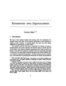
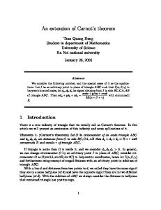
From the proof of the theorem, it follows that the number N is large and thus the strong core may not be an appropriate solution. The size of an economy suitable for the strong core, however, depends on what we are analyzing. In the present paper, we just say that a finite population of agents is more suitable for the strong core than an infinite population of agents. Since the inclusion WEM (E) ⊆ CS (E) holds for any economy E, our theorem says the converse holds if the size of economy is sufficiently large. A small economy E1 can have a strong core allocation f1 that is not an expenditure-minimizing Walrasian allocation. In any replica economy En of E1 , the replica allocation of f1 is not an expenditure-minimizing Walrasian allocation for En . From our theorem, if the number n of replications is sufficiently large, then the replica allocation of f1 is not a strong core allocation for replica economy En , either. The next example illustrates this fact. Example 1. Let L = 2 and T = {s, t}. Each type’s endowment vector is given by es = (3, 1) and et = (2, 2). Each type’s preference relation is represented by the following utility functions (see Figures 1 and 2): 2x(1) + x(2) if x(1) ≤ 1, us (x(1) , x(2) ) = 1 (x(1) + 2x(2) + 3) if x(1) ≥ 2, 2
and
ut (x(1) , x(2) ) = x(1) + x(2) . Clearly, both -s and -t are in P3 . For all n ≥ 1, let An,s = {(s, 1), . . . , (s, n)}, An,t = {(t, 1), . . . , (t, n)}, and An = An,s ∪ An,t . For all n ≥ 1, define economy En : An → T by En (s, i) = s = (-s , es ) and En (t, i) = t = (-t , et ) for all i ∈ {1, . . . , n}. Thus, economy En is the n-fold replica economy of E1 , and economy En consists of n agents of type s and n agents of type t. An allocation f1 : A1 → Z2+ for E1 is defined by f1 (s, 1) = (1, 2) and f1 (t, 1) = (4, 1). One could check that f1 ∈ CS (E1 ) and f1 ̸∈ WEM (E1 ). For all n ≥ 2, let fn : An → Z2+ be a replica allocation of f1 ; that is, fn (s, i) = f1 (s, 1) and fn (t, i) = f1 (t, 1) for all i ∈ {1, . . . , n}. For all n ≥ 2, fn is not an expenditureminimizing Walrasian allocation for En for the same reason as f1 ̸∈ WEM (E1 ). Although f1 is a strong core allocation for E1 , for all n ≥ 2, fn is not a strong core allocation for En as we prove in the following. 14
ommodity 2
es
ommodity 1
0
Figure 1: Endowment vector and indifference curves of agents of type s
ommodity 2
et
ommodity 1
0
Figure 2: Endowment vector and indifference curves of agents of type t
15
Let n ≥ 2. Consider S = {(s, 1), (s, 2), (t, 1)}. Define g : S → Z2+ by g(s, i) = f1 (s, 1) = (1, 2) for i = 1, 2, and g(t, 1) = (6, 0). Then,
∑
g(r, i) =
(r,i)∈S
∑
en (r, i) and g(t, 1) ≻t f1 (t, 1),
(r,i)∈S
where en : An → Z2+ is the endowment allocation for En . Therefore, fn ̸∈ CS (En ) for all n ≥ 2. From our theorem, it follows that there exists an n0 ∈ Z++ such that, for all n ≥ n0 , CS (En ) = WEM (En ) holds. In this example, we can choose n0 = 2. It can be shown that, for all n ≥ 2, CS (En ) = {hn } holds, where hn : An → Z2+ is defined by hn (s, i) = (1, 3) and hn (t, i) = (4, 0) for all i ∈ {1, . . . , n}. Thus, for all n ≥ 2, every allocation in CS (En ) is an expenditure-minimizing Walrasian allocation under the price vector (1, 1). Hence, for all n ≥ 2, ∅ ̸= CS (En ) = WEM (En ). Note that, for all n ≥ 1, endowment allocation en is a Walrasian allocation under the price vector p = (1, p(2) ) with 1 < p(2) < 3/2, but en is not an expenditure-minimizing Walrasian allocation. Summing up these facts, for all n ≥ 2, ∅ = ̸ CS (En ) = WEM (En ) ( W (En ) holds. The next example illustrates that combinatorial condition on the relative ratios #At /#A (t ∈ T ) is needed for the existence of expenditure-minimizing Walrasian equilibrium. Example 2. Consider the type set T from Example 1. In Example 1, we considered economies where the number of agents of type s is equal to the number of agents of type t. Here, we consider economies where these two numbers are different. By an argument similar to Example 1, we can prove that, if economy E : A → T satisfies that 0 < #As /#A ≤ #At /#A, then any exactly feasible allocation f : A → Z2+ such that f (a) = (1, 3) for all a ∈ As , and ∥f (a)∥1 = 4 for all a ∈ At is an expenditure-minimizing Walrasian allocation for E.16 16
For x ∈ RL , ∥x∥1 =
∑L
i=1
|x(i) |.
16
We consider economy E : A → T with #As /#A > #At /#A > 0. If #As /#A ≥ 2/3, then every exactly feasible allocation f : A → Z2+ satisfying f (a) ∈ {(1, 2), (3, 1), (5, 0)} for all a ∈ As , and f (a) = (6, 0) for all a ∈ At is an expenditure-minimizing Walrasian allocation under p = (1, 2). If economy E : A → T satisfies that 2/3 > #As /#A > 1/2, then E does not have an expenditure-minimizing Walrasian equilibrium for the following reason. • Under price vector p = (1, p(2) ) with p(2) < 1, commodity 2 is in excess demand. • Under price vector p = (1, p(2) ) with p(2) > 2, commodity 1 is in excess demand. • Under price vector p = (1, p(2) ) with 1 < p(2) < 2, for agents of type s, the endowment vector es is the unique consumption vector that is individually rational and satisfies the budget constraint with equality. Under such p, es does not satisfy the expenditure minimization. • Under price vector p = (1, p(2) ) with p(2) = 1 or p(2) = 2, preference-maximizing allocations are not feasible, since 2/3 > #As /#A > 1/2.
Summing up these results, we have • If economy E : A → T satisfies that 0 < #As /#A ≤ #At /#A, then WEM (E) ̸= ∅. • If economy E : A → T satisfies that #As /#A ≥ 2/3, then WEM (E) ̸= ∅. • If economy E : A → T satisfies that 2/3 > #As /#A > 1/2, then WEM (E) = ∅. Hence, in order to guarantee the existence of expenditure-minimizing Walrasian equilibrium, the relative ratio of the number of agents of each type to the size of economy is essential. From our theorem, this relative ratio is essential also for the nonemptiness of the strong core. Not only the relative ratios #At /#A (t ∈ T ) but also the type set T is essential for the existence of an expenditure-minimizing Walrasian equilibrium. The next example illustrates this fact. 17
ommodity 2
et
ommodity 1
0
Figure 3: Endowment vector and indifference curves of agents of type t
Example 3. Let L = 2 and T = {t}. Type t’s endowment vector et is given by (1, 2). The preference relation -t of agents of type t is represented by a utility function ut : Z2+ → R defined by
3.5 if (x(1) , x(2) ) = (3, 0), ut (x(1) , x(2) ) = x(1) + x(2) otherwise.
(See Figure 3.) Then, -t ∈ P2 . Although the indifference curves drawn in the figure are not convex, this preference relation is discretely convex in the sense that, for all x ∈ Z2+ , ( ) we have co {y ∈ Z2+ | y %t x} ∩ Z2 = {y ∈ Z2+ | y %t x}, where co(C) denotes the convex hull of set C.17 For all n ≥ 1, let An = {(t, 1), . . . , (t, n)}. Define En : An → T by En (t, i) = t = (-t , et ) for all i ∈ {1, . . . , n}. Let en : An → Z2+ be the endowment allocation for En . In every economy En with n ≥ 1, if price vector p = (1, p(2) ) satisfies that p(2) ≤ 1/2, then commodity 2 is in excess demand; if p = (1, p(2) ) satisfies that p(2) ≥ 1, then commodity 1 is in excess demand. Under price vector p = (1, p(2) ) with 1/2 < p(2) < 1, a pair (p, en ) is a Walrasian equilibrium, but is not an expenditure-minimizing Walrasian 17
The discrete convexity of preference relation is related to the nonemptiness of the weak core. See
Inoue [11].
18
equilibrium. Since any other allocation than en cannot be a Walrasian allocation under p = (1, p(2) ) with 1/2 < p(2) < 1, we have ∅ = WEM (En ) ( W (En ) = {en } for all n ≥ 1. From our theorem, it follows that CS (En ) = ∅ = WEM (En ) for n large enough. Indeed, this equivalence is met for all n ≥ 4; one can prove that CS (En ) = ∅ for all n ≥ 4. On the other hand, if 2 ≤ n ≤ 3, there exists a strong core allocation that is not an expenditureminimizing Walrasian allocation. Actually, endowment allocation e2 for E2 is a strong core allocation, but as mentioned above, e2 is not an expenditure-minimizing Walrasian allocation. Also, an allocation g : {(t, 1), (t, 2), (t, 3)} → Z2+ for E3 defined by g(t, 1) = (3, 0),
and
g(t, i) = (0, 3) for all i ∈ {2, 3} is a strong core allocation but is not a Walrasian allocation for E3 .
3
Outline of the Proof
We give an outline of the proof of the theorem here and give a formal proof in the next section. In order to prove that every strong core allocation is an expenditure-minimizing Walrasian allocation, we need to find a corresponding price vector. The existence of the price vector follows from the separation theorem for convex sets. Let f be a strong core allocation and let ψ(a) = {x ∈ ZL+ | x %a f (a)} − {e(a)}. If we have
( 0 ̸∈ int co
(
∪
)) ψ(a)
,
a∈A
then, by the separation theorem, we obtain a candidate of an equilibrium price vector. We prove this by contradiction. Suppose that ( ( )) ∪ 0 ∈ int co ψ(a) . a∈A
Then, the origin can be a convex combination of some vectors in
∪ a∈A
ψ(a). If all coeffi-
cients of the combination are rational, say, m m ∑ ∑ ∪ λi 0= zi for some λ0 , λ1 , . . . , λm ∈ Z++ with λi = λ0 and some z1 , . . . , zm ∈ ψ(a), λ 0 i=1 i=1 a∈A
19
then the coalition consisting of λ0 agents where, for every i, the net trade vector of each of λi agents is zi weakly improves upon f . To guarantee that all coefficients of the convex combination are rational, we prove in Lemma 1: (1) Strong core allocations are uniformly bounded regardless of the size of an economy. As mentioned later, in the proof of (1), it is essential that the marginal rate of substitution of all agents’ preference relations is uniformly positive in the whole consumption set. Since the bound of strong core allocations does not depend on the size of an economy, the denominator of the rational coefficients of the convex combination is also uniformly bounded regardless of the size of an economy. Even though the coefficients are rational, if net trade vector zi is not preferred for all the λi agents, the coalition cannot weakly improve upon f . Thus, we consider an economy where the number of agents’ types are finite and each type has a sufficiently large number of agents. In such an economy, (2) Strong core allocations have the weak equal treatment property. Namely, consumption vectors assigned to agents of the same type by a strong core allocation are indifferent with respect to the common preference relation. We prove this in Lemma 2. Since agents of the same type have the same preference relation, by the weak equal treatment property, by choosing λi agents from the same type, all the λi agents prefer the net trade vector zi (if one of them prefers) and, therefore, f ( (∪ )) can be weakly improved upon. Consequently, we have 0 ̸∈ int co a∈A ψ(a) . ( (∪ )) By applying the separation theorem to 0 ̸∈ int co a∈A ψ(a) , there exists a price vector p0 ̸= 0 such that, for every a ∈ A, if x %a f (a), then p0 · (x − e(a)) ≥ 0. This price vector p0 satisfies the expenditure minimization, but it does not necessarily satisfy the preference maximization. Thus, we prove in Claim 9: (3) There exists a price vector p under which not only the expenditure minimization but also the preference maximization hold. By slightly moving the vector p0 in an appropriate direction, we can obtain such price vector p. In the proof of (3), we repeatedly use the separation theorem for convex sets. 20
The resulting price vector p, however, need not be a rational vector. Since the commodity space ZL is discrete, by applying Inoue’s [10] separation theorem (Lemma 7 in the Appendix), we prove in the last part of the proof: (4) There exists a rational vector p∗ under which both the expenditure minimization and the preference maximization hold. This is an outline of the proof of the theorem. In the proof of (1), it is essential that agents’ preference relations are in Pk . We exemplify this fact. Let L = 2 and assume that every agent has the same utility function u(x(1) , x(2) ) = x(1) and the same endowment vector e = (1, 1). In this example, an allocation such that one agent’s consumption vector is (1, #A) and the others’ are all (1, 0) is a strong core allocation, but, clearly, the bound of the allocation depends on the size #A of economy. Note that this strong core allocation is an expenditure-minimizing Walrasian allocation under price vector (1, 0), so the uniform positivity of the marginal rate of substitution is essential for our method of proof but it is not always necessary for a strong core allocation to be an expenditure-minimizing Walrasian allocation. Finally, we give the idea of the proof of (2), which is very different from the proof of Debreu and Scarf’s equal treatment property in economies with divisible commodities. Since strong core allocations are uniformly bounded and the number of agents’ types is finite, agents’ net trade vectors f (a) − e(a) are also uniformly bounded. Let ξ be the bound of net trade vectors and let XL,ξ = {x ∈ ZL | ∥x∥∞ ≤ ξ}. This set consists of finitely many integral vectors. For a strong core allocation f and every x ∈ XL,ξ , let α(x) be the number of agents whose net trade vectors are exactly x. Since f is exactly feasible, we have ∑
α(x)x = 0.
x∈XL,ξ
If the size of economy is large, that is, if the number
∑ x∈XL,ξ
α(x) is large, there exists a
subset of agents such that the summation of their net trade vectors is zero. Namely, there exists β : XL,ξ → Z+ such that β(x) ≤ α(x) for all x ∈ XL,ξ with at least one x ∈ XL,ξ 21
the inequality being strict, and
∑ x∈XL,ξ
∑
β(x)x = 0. This follows from Lemma 3 in the
β(x) agents such that, for every x ∈ XL,ξ , ∑ the number of agents with net trade vector x is β(x). From x∈XL,ξ β(x)x = 0, it follows
Appendix. Let S be a coalition with
that
∑
x∈XL,ξ
(f (a) − e(a)) = 0.
a∈S
Since f is exactly feasible, we also have ∑
(f (a) − e(a)) = 0.
a∈A\S
We prove the weak equal treatment property of strong core allocations by contradiction. Suppose that f does not have the weak equal treatment property. Then, there exists a type t and two distinct agents a∗ and b∗ of type t with f (a∗ ) ≻t f (b∗ ). A weakly improving coalition is based on S or A\S. We remove agent a∗ with higher utility consumption vector from the coalition and add one agent of the same type with lower utility consumption vector. In the weakly improving allocation, the added agent consumes the higher utility consumption vector f (a∗ ). The allocation is exactly feasible within the coalition, because the removed and the added agents are of the same type and the summation of net trade vectors among agents in S or in A \ S is zero.
4
Proof of Theorem
Let r ∈ R with r ≥ 1, k ∈ Z with k ≥ 2, and T ⊆ Pk × ZL+ with #T ≤ r and
∑ t∈T
et ≫ 0.
Let M = max{∥e∥∞ | (-, e) ∈ T } and ξ = max{rM 2 L2 (M L + 1), (kL + 1)M L}. Note that the number ξ depends only on exogenous variables. We will prove that strong core allocations are uniformly bounded regardless of the size of economy. In the case of perfectly divisible commodities, Bewley [4, Theorem 1] first proved that strong core allocations are uniformly bounded. His proof uses a contradiction argument, so the bound of strong core allocations is not clear. On the other hand, Mas-Colell’s [16, Lemma 7.4.10] proof clarifies the bound. Our proof is based on Mas-Colell’s proof. 22
Lemma 1. For every finite set A of agents, if economy E : A → T satisfies that #At /#A ≥ 1/r for all t ∈ T , then ∥f (a)∥∞ ≤ ξ for all f ∈ CS (E) and all a ∈ A. Proof. Let A be the set of agents and E : A → T be an economy such that #At /#A ≥ 1/r for all t ∈ T . Let f ∈ CS (E). By a simple calculation, it follows that, if #A ≤ rM L2 (M L+ 1), then ∥f (a)∥∞ ≤ ξ for all a ∈ A. Therefore, in the remainder of the proof, we assume that #A > rM L2 (M L + 1). Let J = {j ∈ {1, . . . , L} | f (j) (a) ≥ M L + 1 for some a ∈ A} and J ′ = {j ∈ {1, . . . , L} | f (j) (a) ≥ (kL + 1)M L for some a ∈ A}. Then, J ′ ⊆ J. If J = ∅, the proof has been completed. Thus, the set J is supposed to be nonempty. For j ∈ J, we choose aj ∈ argmax{f (j) (a) | a ∈ A}. Note that ai = aj may hold for some distinct indices i and j in J. Let B = {aj | j ∈ J}. Then, #B ≤ #J ≤ L. ∑ The excess demand of the coalition B is denoted by y = a∈B (f (a) − e(a)) ∈ ZL . Let J ′′ = {j ∈ {1, . . . , L} | y (j) ≤ −1}. By a simple calculation, y (j) ≥ 1 for all j ∈ J. Thus, J ∩ J ′′ = ∅. We also have: (1) y (j) ≥ kM L2 for all j ∈ J ′ . In addition, if J ′ = ∅, then ∥f (a)∥∞ ≤ ξ for all a ∈ A. Therefore, the proof is completed if we can prove that J ′ = ∅. Claim 1. J ′ = ∅. Proof. Suppose, to the contrary, that J ′ ̸= ∅. Let C = A \ B. Then, #C = #A − #B ≥ #A − L. Since #A > rM L2 (M L + 1) > L, we have C ̸= ∅. Define ye ∈ ZL by ye = y −
∑
y (j) χj .
j∈J ′′
Clearly, ye ≥ 0. Moreover, from (1), it follows that, for all j ∈ J ′ , ye(j) = y (j) ≥ kM L2 . Subclaim 1.1. J ′′ ̸= ∅. Proof. Suppose, to the contrary, that J ′′ = ∅. We have kM L2
∑ j∈J ′
χj ≤ ye = y ∑ = a∈B (f (a) − e(a)) ∑ = − a∈C (f (a) − e(a)) ∑ = a∈C (e(a) − f (a)). 23
The third equality follows from the exact feasibility of strong core allocation f . Since C ̸= ∅, we can choose an agent a∗ of C. Define a mapping g : C → ZL+ by f (a∗ ) + ∑ (e(c) − f (c)) if a = a∗ , c∈C g(a) = f (a) if a ∈ C \ {a∗ }. Because g(a∗ ) ≥ f (a∗ ) + kχj for all j ∈ J ′ and -a∗ ∈ Pk , we have g(a∗ ) ≻a∗ f (a∗ ). We also have
∑
g(a) =
a∈C
∑ a∈C
f (a) +
∑
(e(c) − f (c)) =
c∈C
∑
e(a).
a∈C
This contradicts that f ∈ CS (E). Thus, we have established the proof of Subclaim 1.1.
For all j ∈ J ′′ , let Cj = {a ∈ C | f (j) (a) ≥ 1}. Subclaim 1.2. #Cj > M L2 for all j ∈ J ′′ . Proof. Let j ∈ J ′′ . Since J ∩ J ′′ = ∅, it follows that j ̸∈ J. Thus, f (j) (a) ≤ M L for all a ∈ A. Since C \ Cj = {a ∈ C | f (j) (a) < 1} = {a ∈ C | f (j) (a) = 0}, we have ∑
f (j) (a) ≤ {#A − (#C − #Cj )}M L
a∈A
= (#Cj )M L + (#A − #C)M L ≤ (#Cj )M L + M L2 . On the other hand, since Thus,
∑
(j)
t∈T
et ≫ 0, there exists a type tj ∈ T such that etj ≥ 1.
∑ ∑ #A e(j) (a). ≤ #Atj ≤ e(j) (a) ≤ r a∈A a∈A tj
Because strong core allocation f is exactly feasible, we have ∑ #A ∑ (j) ≤ e (a) = f (j) (a) ≤ (#Cj )M L + M L2 . r a∈A a∈A Thus, #Cj ≥
#A rM L2 (M L + 1) −L> − L = M L2 . rM L rM L
This completes the proof of Subclaim 1.2.
24
For all j ∈ J ′′ , we have −1 ≥ y (j) =
∑
≥ −
(j)
a∈B (f
∑
(a) − e(j) (a))
e(j) (a)
a∈B
≥ −M (#B) ≥ −M L. Therefore, by Subclaim 1.2, there exists {Gj | j ∈ J ′′ } such that Gj ⊆ Cj
for all j ∈ J ′′ ,
#Gj = −y (j) for all j ∈ J ′′ , and Gj ∩ Gℓ = ∅
if j ̸= ℓ.
Since J ′ ̸= ∅, by (1), there exists an h ∈ {1, . . . , L} such that ye(h) = y (h) ≥ kM L2 . Define a mapping gb : C → ZL by f (a) + kχ − χ if a ∈ G and j ∈ J ′′ , h j j gb(a) = ∪ f (a) if a ∈ C \ j∈J ′′ Gj . For all a ∈ Gj , f (j) (a) ≥ 1 holds since Gj ⊆ Cj . Thus, gb(a) ∈ ZL+ for all a ∈ C. Because ∪ -a ∈ Pk for all a ∈ C, we have gb(a) ≻a f (a) for all a ∈ j∈J ′′ Gj . We also have ∑ ∑ ∑ ∑ gb(a) = f (a) + k (#Gj )χh − (#Gj )χj a∈C
j∈J ′′
a∈C
=
∑
(
f (a) − k
≤
f (a) + kM L2 χh +
a∈C
≤
∑
f (a) + ye +
=
∑
f (a) +
a∈C
=
∑
=
f (a) −
=
∑
e(a)
e(a) −
∑
e(a)
a∈B
e(a).
a∈C
25
∑ j∈J ′′
y (j) χj
j∈J ′′
y (j) χj
(f (a) − e(a))
a∈B
a∈A
∑
∑ a∈B
a∈A
∑
∑
f (a) + y
a∈C
=
∑
χh +
j∈J ′′
a∈C
∑
y (j)
j∈J ′′
a∈C
∑
∑
j∈J ′′
)
y (j) χj
Although gb may not be exactly feasible within coalition C, coalition C can weakly improve upon f because agents’ preference relations are weakly monotone. This contradicts that f ∈ CS (E). This completes the proof of Claim 1. Thus, we have established the proof of Lemma 1.
Next, we prove that in an economy with a large number of agents, every strong core allocation has the weak equal treatment property. Before giving the precise statement, we introduce some notation. Let XL,ξ = {x ∈ ZL | ∥x∥∞ ≤ ξ}. A set XL,ξ is defined ∑ as follows. A mapping α : XL,ξ → Z+ belongs to XL,ξ if and only if x∈XL,ξ α(x) ≥ 1, ∑ x∈XL,ξ α(x)x = 0, and there exists no mapping β : XL,ξ → Z+ such that ∑
β(x) ≥ 1,
x∈XL,ξ
∑
β(x)x = 0,
x∈XL,ξ
β(x) ≤ α(x) for all x ∈ XL,ξ , and β(y) < α(y) for some y ∈ XL,ξ . ∑
µ(L, ξ) = sup α(x) α ∈ XL,ξ . x∈XL,ξ
Let
The important fact is that µ(L, ξ) is finite and, therefore, it is a natural number. This fact is proved in Lemma 3 in the Appendix. The first statement of the theorem follows from the following lemma. Lemma 2. Let A be the set of agents such that #A > rµ(L, ξ). If economy E : A → T satisfies that #At /#A ≥ 1/r for all t ∈ T , then all strong core allocations for E have the weak equal treatment property, i.e., for all f ∈ CS (E), all t ∈ T , and all a, b ∈ At , we have f (a) ∼t f (b). Proof. Suppose, to the contrary, that there exists an allocation f ∈ CS (E), a type t ∈ T , and two agents a, b ∈ At such that f (a) ≻t f (b). Without loss of generality, we can assume that f (a) %t f (c) %t f (b) for all c ∈ At . By Lemma 1, ∥f (c)∥∞ ≤ ξ for all c ∈ A. Since both f (c) and e(c) are nonnegative vectors, we have ∥f (c) − e(c)∥∞ ≤ max{ξ, M } = ξ
26
for all c ∈ A. Thus, f (c) − e(c) ∈ XL,ξ for all c ∈ A. Define α : XL,ξ → Z+ by, for all x ∈ XL,ξ , α(x) = #{c ∈ A | f (c) − e(c) = x}. Note that ∑
α(x)x =
x∈XL,ξ
∑
∑
(f (c) − e(c)) = 0 and
c∈A
α(x) = #A > rµ(L, ξ).
x∈XL,ξ
Thus, by the definition of µ(L, ξ), there exists a natural number ℓ > r and βj ∈ XL,ξ ∑ (j = 1, . . . , ℓ) such that for all x ∈ XL,ξ , α(x) = ℓj=1 βj (x). Therefore, there exists a partition {B1 , . . . , Bℓ } of A such that for all j ∈ {1, . . . , ℓ} and all x ∈ XL,ξ , βj (x) = #{c ∈ Bj | f (c) − e(c) = x}. Without loss of generality, we can assume b ∈ B1 . Since β1 ∈ XL,ξ , we have ∑
∑
(f (c) − e(c)) =
c∈B1
#B1 =
∑
β1 (x)x = 0 and
x∈XL,ξ
β1 (x) ≤ µ(L, ξ).
x∈XL,ξ
Note that the set At \ B1 is nonempty, because #At ≥ #A/r > µ(L, ξ) ≥ #B1 . Claim 2. f (c) ∼t f (b) for all c ∈ At \ B1 . Proof. Suppose, to the contrary, that f (c∗ ) ≻t f (b) for some c∗ ∈ At \ B1 . We consider a coalition C1 = (A \ (B1 ∪ {c∗ })) ∪ {b}. Define g1 : C1 → ZL+ by f (c∗ ) if c = b, g1 (c) = f (c) if c ∈ C1 \ {b}. Since ∑
∑
c∈A\B1 (f (c)
c∈C1 (g1 (c)
− e(c)) = 0 and agents b and c∗ are of the same type, we have
− e(c)) = 0. In addition, we have g1 (b) = f (c∗ ) ≻t f (b). This contradicts
that f ∈ CS (E). This completes the proof of Claim 2.
27
From Claim 2, it follows that a ∈ B1 . Since At \B1 is nonempty, we can pick c′ ∈ At \B1 . We consider a coalition C2 = (B1 \ {a}) ∪ {c′ }. Define g2 : C2 → ZL+ by f (a) if c = c′ , g2 (c) = f (c) if c ∈ C2 \ {c′ }. Since ∑
∑
c∈B1 (f (c)
c∈C2 (g2 (c)
− e(c)) = 0 and agents a and c′ are of the same type, we have
− e(c)) = 0. In addition, from Claim 2, it follows that g2 (c′ ) = f (a) ≻t
f (b) ∼t f (c′ ). This contradicts that f ∈ CS (E). This completes the proof of Lemma 2.
We next prove the second statement of the theorem. Let ρ = ξ + k(L − 1)ξ
and
q = max{µ(L, ξ), 2L−1 LL/2 ρL+1 (1 + ρ)}.
Note that both numbers ρ and q depend only on exogenous variables. Let A be the set of agents such that #A > rq and let E : A → T be an economy such that #At /#A ≥ 1/r for all t ∈ T . We prove that CS (E) ⊆ WEM (E). (Recall that the opposite inclusion WEM (E) ⊆ CS (E) is always satisfied.) Let f ∈ CS (E). Claim 3. ρ χi ≻a f (a) for all i ∈ {1, . . . , L} and all a ∈ A. Proof. Let i ∈ {1, . . . , L} and a ∈ A. We consider two distinct cases. Case 1. f (j) (a) = 0 for all j ̸= i. Since -a ∈ Pk , we have ( ) f (a) ≺a f (a) + k χi = f (i) (a) + k χi . By Lemma 1, we have f (i) (a) + k ≤ ξ + k < ρ. Since -a is weakly monotone, we have f (a) ≺a ρ χi . Case 2. f (j) (a) ≥ 1 for some j ̸= i. 28
Since -a ∈ Pk , we have f (a) ≺a f (a) −
∑
f (j) (a)χj + k
j̸=i
∑
( f (j) (a)χi =
f (i) (a) + k
j̸=i
∑
) f (j) (a) χi .
j̸=i
By Lemma 1, we have f (i) (a) + k
∑
f (j) (a) ≤ ξ + k(L − 1)ξ = ρ.
j̸=i
Since -a is weakly monotone, we have f (a) ≺a ρ χi . This completes the proof of Claim 3.
For every t ∈ T , let φt = {z ∈ ZL | z + et ∈ ZL+
and z + et ≻t f (a)} = {x ∈ ZL+ | x ≻t f (a)} − {et }
ψt = {z ∈ ZL | z + et ∈ ZL+
and z + et %t f (a)} = {x ∈ ZL+ | x %t f (a)} − {et },
and
where a ∈ At . By Lemma 2, since #A > rµ(L, ξ), φt and ψt are both well defined for all t ∈ T . For all t ∈ T , define the set φ′t of minimal elements of φt as follows: z ∈ φ′t if and only if z ∈ φt and there exists no y ∈ φt with y < z. The set ψt′ of minimal elements of ψt is defined similarly. Since every φt and every ψt is bounded from below, by Gordan’s lemma (Lemma 4 in the Appendix), φ′t and ψt′ are nonempty and finite, and satisfies that φt ⊆ φ′t + ZL+ and ψt ⊆ ψt′ + ZL+ . Since agents’ preference relations are weakly monotone, we have φt = φ′t + ZL+ and ψt = ψt′ + ZL+ for all t ∈ T . Let XL,ρ = {x ∈ ZL | ∥x∥∞ ≤ ρ}. Claim 4. φ′t ⊆ XL,ρ and ψt′ ⊆ XL,ρ for all t ∈ T . Proof. We only prove that φ′t ⊆ XL,ρ . The inclusion ψt′ ⊆ XL,ρ can be proved similarly. Suppose, to the contrary, that φ′t ̸⊆ XL,ρ for some t ∈ T . Since φ′t ⊆ ZL+ − {et } ⊆ ZL+ − {(M, . . . , M )} and M < ρ, we have, for all z ∈ φ′t and all h ∈ {1, . . . , L}, z (h) > −ρ. Therefore, from φ′t ̸⊆ XL,ρ , there exists a z ∈ φ′t and an h ∈ {1, . . . , L} such that z (h) > ρ.
29
Since ρ χh ≻t f (a) for all a ∈ At by Claim 3, we have ρ χh − et ∈ φt . For coordinate h, we have (h)
(h)
z (h) > ρ ≥ ρ χh − et . Since z ≥ −et , for coordinate i with i ̸= h, we have (i)
(i)
(i)
z (i) ≥ −et = ρ χh − et . Thus, z > ρ χh − et and ρ χh − et ∈ φt . This contradicts that z ∈ φ′t . We have established the proof of Claim 4.
By Claim 4, for all t ∈ T , we have ψt = ψt′ + ZL+ = (ψt′ ∩ XL,ρ ) + ZL+ ⊆ (ψt ∩ XL,ρ ) + ZL+ ⊆ ψt + ZL+ = ψt . Thus, ψt = (ψt ∩ XL,ρ ) + ZL+ for all t ∈ T . Therefore,
∪ t∈T
ψt =
(∪ t∈T
) ψt ∩ XL,ρ + ZL+ .
( (∪ )) ( (∪ )) Claim 5. 0 ̸∈ int co t∈T ψt if and only if 0 ̸∈ int co t∈T ψt ∩ XL,ρ , where int(C) and co(C) denote the interior and the convex hull of set C, respectively. )) ( (∪ Proof. It suffices to prove the sufficiency. Assume that 0 ̸∈ int co t∈T ψt ∩ XL,ρ . By the separation theorem for convex sets, there exists a p ∈ RL \ {0} such that, for all (∪ ) z ∈ co t∈T ψt ∩ XL,ρ , p · z ≥ 0. We prove that p ≥ 0. Let i ∈ {1, . . . , L}. Since, by Claim 3, ρ χi ≻t f (a) for all a ∈ At and all t ∈ T , and since et ≥ 0 and -t is weakly monotone, we have ρ χi + et %t ρ χi ≻t f (a). Thus, ρ χi ∈ φt ∩ XL,ρ ⊆ ψt ∩ XL,ρ . Then, by the consequence of the separation theorem for convex sets, 0 ≤ p · (ρ χi ) = ρ p(i) . 30
Thus, p(i) ≥ 0. We have then p ≥ 0. ) (∪ ) (∪ ∪ L Since t∈T ψt = t∈T ψt . t∈T ψt ∩ XL,ρ + Z+ , we have p · z ≥ 0 for all z ∈ co ( (∪ )) Hence, 0 ̸∈ int co t∈T ψt . This completes the proof of Claim 5.
We next find a price vector p under which strong core allocation f satisfies both the expenditure minimization and the preference maximization. To obtain such price vector p, we first find a price vector p0 under which f satisfies the expenditure minimization. Then, we move p0 in an appropriate direction slightly and make the resulting price vector satisfy the desired properties. The following claim will be used not only when we find the first price vector p0 but also when we move p0 in an appropriate direction. ∪ Claim 6. Let H be a linear subspace of RL . If t∈T φt ∩ XL,ρ ∩ H ̸= ∅, then 0 ̸∈ ( (∪ )) ri co t∈T ψt ∩ XL,ρ ∩ H , where ri(C) denotes the relative interior of set C. ( (∪ )) ∪ Proof. Suppose, to the contrary, that 0 ∈ ri co t∈T ψt ∩ XL,ρ ∩ H . Let z0 ∈ t∈T φt ∩ XL,ρ ∩H. Then, there exists a t0 ∈ T with z0 ∈ φt0 . Since ≻t0 is irreflexive and f (a) %t0 et0 ) (∪ for every a ∈ At0 , we have z0 ̸= 0. Let s = min{s ∈ R | s z0 ∈ co t∈T ψt ∩ XL,ρ ∩ H }. Then, by Lemma 6 in the Appendix, |s| ≤ ρ and there exist q0 ∈ Z++ with q0 ≤ (1)
(mt )
2L−1 LL/2 ρL+1 , {xt,j | j = 1, . . . , mt } ⊆ ψt ∩ XL,ρ ∩ H (t ∈ T ), and (αt , . . . , αt
t ) ∈ Qm +
(t ∈ T ) such that 0 ≤ mt ≤ L for all t ∈ T , ∑ 1≤ mt ≤ L, t∈T
mt ∑∑
(j)
αt = 1,
t∈T j=1 (j) q0 α t ∈
Z+
for all j ∈ {1, . . . , mt } and all t ∈ T ,
q0 s ∈ −Z++ , and mt ∑∑ (j) αt xt,j = s z0 . t∈T j=1
Since #A > rq = r max{µ(L, ξ), 2L−1 LL/2 ρL+1 (1 + ρ)}, we have, for all t ∈ T , #At ≥ ∑ t (j) #A/r > 2L−1 LL/2 ρL+1 (1 + ρ) > q0 ≥ m j=1 q0 αt . Thus, for all t ∈ T \ {t0 }, there exists a mutually disjoint family {Ct,j | j = 1, . . . , mt } of subsets of At such that (j)
#Ct,j = q0 αt
for all j ∈ {1, . . . , mt }. 31
Since q0 + q0 s ≤ 2L−1 LL/2 ρL+1 (1 + ρ) < #At0 , there exists a mutually disjoint family {Ct0 ,j | j = 1, . . . , mt0 } ∪ {D} of subsets of At0 such that (j)
#Ct0 ,j = q0 αt0
for all j ∈ {1, . . . , mt0 }, and
#D = q0 |s|. Let S =
∪mt
∪ t∈T
j=1
Ct,j ∪ D. Define g : S → ZL+ by
x + e if a ∈ C , t ∈ T , and j ∈ {1, . . . , m }, t,j t t,j t g(a) = z +e if a ∈ D. 0 t0 Then, ∑
mt ∑∑
g(a) =
(#Ct,j ) xt,j + (#D) z0 +
t∈T j=1
a∈S
(
= q0 ∑
=
mt ∑∑
(j)
t∈T j=1
e(a)
a∈S
) αt xt,j + |s| z0
∑
+
∑
e(a)
a∈S
e(a).
a∈S
Therefore, g is exactly feasible within coalition S. For a ∈ Ct,j with t ∈ T and j ∈ {1, . . . , mt }, since xt,j ∈ ψt , we have g(a) = xt,j + et %t f (a). For a ∈ D, since z0 ∈ φt0 , we have g(a) = zt0 + et0 ≻t0 f (a). This contradicts that f ∈ CS (E). Hence, 0 ̸∈ ( (∪ )) ri co t∈T ψt ∩ XL,ρ ∩ H . This completes the proof of Claim 6. ( (∪ )) φt ∩ XL,ρ ̸= ∅ and then, by Claim 6, 0 ̸∈ int co t∈T ψt ∩ XL,ρ . ( (∪ )) Thus, by Claim 5, we have 0 ̸∈ int co t∈T ψt . By the separation theorem for convex (∪ ) sets, there exists a p0 ∈ RL \ {0} such that p0 · z ≥ 0 for all z ∈ co t∈T ψt . From the (∪ ) (∪ ) weak monotonicity of preference relations, co t∈T ψt = co t∈T ψt + RL+ . Hence, we By Claim 4,
∪
t∈T
have p0 ≥ 0. Claim 7. p0 · (f (a) − e(a)) = 0 for all a ∈ A. Proof. Since f (a) − e(a) ∈
∪ t∈T
ψt for all a ∈ A, we have p0 · (f (a) − e(a)) ≥ 0. By the
exact feasibility of f , we have p0 · (f (a) − e(a)) = 0 for all a ∈ A.
32
Claim 8. p0 ≫ 0. (h)
Proof. Suppose, to the contrary, that there exists an h ∈ {1, . . . , L} with p0 = 0. ∑ (j) Since p0 ∈ RL+ \ {0}, there exists a j ∈ {1, . . . , L} with p0 > 0. Since a∈A f (j) (a) = ∑ (j) (j) (a) ≥ 1. From -a ∈ Pk , it follows a∈A e (a) > 0, there exists an agent a ∈ A with f that f (a) ≺a f (a) − χj + k χh . Thus, f (a) − χj + k χh − e(a) ∈
∪
φt ⊆
t∈T
∪
ψt .
t∈T
By the consequence of the separation theorem and by Claim 7, we have (j)
(h)
(j)
0 ≤ p0 · (f (a) − χj + k χh − e(a)) = −p0 + k p0 = −p0 , which is a contradiction. Thus, p0 ≫ 0.
Claim 9. There exists a p ∈ RL++ such that (1) p · z > 0 for all z ∈ (2) p · z ≥ 0 for all z ∈
∪ t∈T
∪ t∈T
φt , and ψt .
∪ Proof. Let H0 = {z ∈ RL | p0 · z = 0}. If t∈T φt ∩ H0 = ∅, then p0 satisfies the desired ∪ properties. Assume that t∈T φt ∩ H0 ̸= ∅. Subclaim 9.1.
∪ t∈T
ψt ∩ H0 ⊆ XL,ρ .
∪ Proof. Let z ∈ t∈T ψt ∩ H0 . Then, p0 · z = 0. Since, by Claim 8, p0 ≫ 0 and p0 · y ≥ 0 ) (∪ ∪ for all y ∈ co t∈T ψt , we have z ∈ t∈T ψt′ . By Claim 4, z ∈ XL,ρ .
By Subclaim 9.1, we have ∅ ̸=
∪ t∈T
Thus,
∪ t∈T
φ t ∩ H0 ⊆
∪
ψt ∩ H0 ⊆ XL,ρ .
t∈T
φt ∩ XL,ρ ∩ H0 ̸= ∅ and, by Claim 6, we have ( ( )) ( ( )) ∪ ∪ 0 ̸∈ ri co ψt ∩ XL,ρ ∩ H0 = ri co ψt ∩ H0 . t∈T
t∈T
33
By the separation theorem for convex sets, there exists a p1 ∈ span ∪ such that p1 · z ≥ 0 for all z ∈ t∈T ψt ∩ H0 . Let { } ∪ ∪ E0 = ψt \ H0 = z ∈ ψt p0 · z > 0 . t∈T
(∪ t∈T
) ψt ∩ H0 \ {0}
t∈T
Let E0′ be the set of minimal elements of E0 , i.e., x ∈ E0′ if and only if x ∈ E0 and there exists no y ∈ E0 with y < x. Since E0 is nonempty and bounded from below, by Gordan’s lemma (Lemma 4 in the Appendix), E0′ is a nonempty finite subset of E0 and satisfies that E0 ⊆ E0′ + ZL+ . Since p0 ≫ 0, we have 0 < min{p0 · z | z ∈ E0′ } = inf{p0 · z | z ∈ E0 }. Since the mapping p 7→ min{p·z | z ∈ E0′ } is continuous, there exists an open neighborhood U0 of p0 such that, for all p ∈ U0 , min{p · z | z ∈ E0′ } > 0. Since p0 ≫ 0, by taking a sufficiently small ε1 > 0, we have p0 + ε1 p1 ≫ 0 and p0 + ε1 p1 ∈ U0 . Then, 0 < min{(p0 + ε1 p1 ) · z | z ∈ E0′ } = inf{(p0 + ε1 p1 ) · z | z ∈ E0 }. Summing up, we have obtained that (a) p0 + ε1 p1 ∈ RL++ ; (b) (p0 + ε1 p1 ) · z > 0 for all z ∈ (c) (p0 + ε1 p1 ) · z ≥ 0 for all z ∈
∪ t∈T
∪ t∈T
ψt \ H0 ; and ψt ∩ H0 .
∪ Let H1 = {z ∈ RL | (p0 + ε1 p1 ) · z = 0}. If t∈T φt ∩ H0 ∩ H1 = ∅, then p0 + ε1 p1 ∪ satisfies the desired properties. Assume that t∈T φt ∩ H0 ∩ H1 ̸= ∅. Then, by the same (∪ ) argument as above, there exists a p2 ∈ span t∈T ψt ∩ H0 ∩ H1 \ {0} and an ε2 > 0 such that (a′ ) p0 + ε1 p1 + ε2 p2 ∈ RL++ ; (b′ ) (p0 + ε1 p1 + ε2 p2 ) · z > 0 for all z ∈ (c′ ) (p0 + ε1 p1 + ε2 p2 ) · z ≥ 0 for all z ∈
∪ t∈T
∪
34
t∈T
ψt \ (H0 ∪ H1 ); and ψt ∩ H0 ∩ H1 .
∪ Let H2 = {z ∈ RL | (p0 + ε1 p1 + ε2 p2 ) · z = 0}. If t∈T φt ∩ H0 ∩ H1 ∩ H2 = ∅, then ∪ p0 + ε1 p1 + ε2 p2 satisfies the desired properties. If t∈T φt ∩ H0 ∩ H1 ∩ H2 ̸= ∅, then, by repeating the same argument, say, m times (m ≤ L), we could obtain that ∪ φt ∩ H0 ∩ H1 ∩ · · · ∩ Hm−1 = ∅, because 0 ̸∈
∪ t∈T
t∈T
φt and
dim (H0 ∩ H1 ∩ H2 ) < dim (H0 ∩ H1 ) < dim H0 = L − 1. ∑ The vector p0 + m−1 i=1 εi pi satisfies the desired properties. This completes the proof of Claim 9.
Let p be the vector obtained in Claim 9. Let { } { } ∪ ∪ F = z∈ ψt p · z > 0 and V = span z ∈ ψt p · z = 0 . t∈T t∈T ∪ Since f (a) − e(a) ∈ t∈T ψt for all a ∈ A, we have, by Claim 9, p · (f (a) − e(a)) ≥ 0 for all a ∈ A. By the exact feasibility of f , we have p · (f (a) − e(a)) = 0 for all a ∈ A and, therefore, f (a) − e(a) ∈ V for all a ∈ A. Thus, by Claim 9, the pair (p, f ) satisfies conditions (i)-(iii) of the definition of expenditure-minimizing Walrasian equilibrium, but p may not be a rational vector. Finally, we find an integral price vector p∗ under which f is an expenditure-minimizing Walrasian allocation. Note that co(F ) ∩ V = ∅. Since p ≫ 0, we have co(F + ZL+ ) ∩ V = ∅ and, then, co(F ) ∩ (V − RL+ ) = ∅. By Inoue’s [10] separation theorem (Lemma 7 in the Appendix), there exists a p∗ ∈ V ⊥ ∩ ZL+ and an ε > 0 such that p∗ · z ≥ ε for all z ∈ F . We prove that (p∗ , f ) is an expenditure-minimizing Walrasian equilibrium. Since p∗ ∈ V ⊥ and f (a) − e(a) ∈ V for all a ∈ A, we have p∗ · (f (a) − e(a)) = 0 for all a ∈ A. Let a ∈ A and x ∈ ZL+ with x ≻a f (a). Then, x − e(a) ∈ p∗ · (x − e(a)) ≥ ε > 0. Let a ∈ A and x ∈ ZL+ with x %a f (a). Then, x − e(a) ∈
∪
∪ t∈T
t∈T
φt ⊆ F . Thus,
ψt ⊆ F ∪ V . Thus,
p∗ · (x − e(a)) ≥ 0. Therefore, (p∗ , f ) is an expenditure-minimizing Walrasian equilibrium. We have established that CS (E) ⊆ WEM (E). 35
Appendix The following results are used in the proof of the theorem. Lemma 3. Let L and N be natural numbers. Let XL,N = {x ∈ ZL | ∥x∥∞ ≤ N }. Define a set XL,N as follows: A mapping α : XL,N → Z+ belongs to XL,N if and only if ∑ ∑ x∈XL,N α(x) ≥ 1, x∈XL,N α(x)x = 0, and there exists no mapping β : XL,N → Z+ such ∑ ∑ that x∈XL,N β(x) ≥ 1, x∈XL,N β(x)x = 0, β(x) ≤ α(x) for all x ∈ XL,N , and β(y) < α(y) for some y ∈ XL,N . Then, the number ∑ µ(L, N ) := sup α(x) α ∈ XL,N x∈XL,N is finite. Hence, µ(L, N ) can be achieved by some α ∈ XL,N . In particular, µ(1, 1) = 2, µ(1, N ) ≤ N 2 (N + 1)/2
for all N ≥ 2, and
µ(L + 1, N ) ≤ µ(L, N )µ(1, N (N + 1)µ(L, N ))
for all L, N ∈ Z++ .
Proof. We prove the lemma by induction on L. Let L = 1. Clearly, µ(1, 1) = 2. We consider the case where N ≥ 2. Claim 10. µ(1, N ) ≤ N 2 (N + 1)/2 for all N ≥ 2. ∑ Proof. Suppose, to the contrary, that there exists a mapping α ∈ X1,N such that x∈X1,N α(x) > ∑ N 2 (N + 1)/2. Because x∈X1,N α(x) > 2, by the definition of X1,L , α(0) = 0 and there exists no ℓ ∈ X1,N \ {0} such that α(ℓ) ≥ 1 and α(−ℓ) ≥ 1. Thus, #{x ∈ X1,N | α(x) ≥ ∑ 1} ≤ N . Since x∈X1,N α(x) > N 2 (N + 1)/2, there exists an integer m ∈ X1,N \ {0} such that α(m) > N (N + 1)/2. We may assume that m ≥ 1. Subclaim 10.1. If ℓ ∈ Z and 1 ≤ ℓ ≤ N , then α(−ℓ) < m. Proof. Suppose, to the contrary, that there exists an ℓ ∈ Z such that 1 ≤ ℓ ≤ N and α(−ℓ) ≥ m. Note that α(m) > N (N +1)/2 > N ≥ ℓ. We define a mapping β : X1,N → Z+
36
by
m if x = −ℓ, β(x) = ℓ if x = m, 0 otherwise.
Clearly,
∑
β(x) ≥ 1,
x∈X1,N
β(x) ≤ α(x) for all x ∈ X1,N , and Moreover, we have
β(m) < α(m).
∑
x∈X1,N
β(x)x = m(−ℓ) + ℓm = 0. This contradicts that α ∈ X1,N .
Therefore, we have established the proof of Subclaim 10.1.
Since 0= we have
∑N ℓ=1
∑
α(x)x =
x∈X1,N
α(−ℓ)ℓ =
∑N
ℓ=1
N ∑
α(ℓ)ℓ +
N ∑
α(−ℓ)(−ℓ),
ℓ=1
ℓ=1
α(ℓ)ℓ. On the other hand, from Subclaim 10.1, it follows
that N ∑
α(−ℓ)ℓ < m
N ∑
ℓ
ℓ=1
ℓ=1
= mN (N + 1)/2 < α(m)m N ∑ ≤ α(ℓ)ℓ, ℓ=1
which is a contradiction. This completes the proof of Claim 10.
Let K ∈ Z++ . Assume that for all N ∈ Z++ and all L ∈ Z++ with L ≤ K, µ(L, N ) is finite. We now prove that µ(K + 1, N ) is finite for all N ∈ Z++ . Claim 11. µ(K + 1, N ) ≤ µ(K, N )µ(1, N (N + 1)µ(K, N )) for all N ∈ Z++ . Proof. Suppose, to the contrary, that µ(K + 1, N ) > µ(K, N )µ(1, N (N + 1)µ(K, N )) for some N ∈ Z++ . Then, there exists a mapping α ∈ XK+1,N such that ∑ α(x) > µ(K, N )µ(1, N (N + 1)µ(K, N )). x∈XK+1,N
37
We define a mapping β : XK,N → Z+ by β(y) =
∑ ℓ∈X1,N
α(ℓ, y) for all y ∈ XK,N . From
α ∈ XK+1,N , it follows that ∑ y∈XK,N
∑
∑
β(y)y =
α(ℓ, y)y = 0.
y∈XK,N ℓ∈X1,N
We also have ∑
β(y) =
y∈XK,N
∑
∑
α(ℓ, y)
y∈XK,N ℓ∈X1,N
∑
=
α(x)
x∈XK+1,N
> µ(K, N )µ(1, N (N + 1)µ(K, N )). Thus, there exists a natural number k > µ(1, N (N + 1)µ(K, N )) and mappings γ ej ∈ ∑k ∑k XK,N (j = 1, . . . , k) such that, for all y ∈ XK,N , j=1 γ ej (y) = β(y). Since j=1 γ ej (y) = ∑ ℓ∈X1,N α(ℓ, y) for all y ∈ XK,N , there exist mappings γj : XK+1,N → Z+ (j = 1, . . . , k) such that ∑
γj (ℓ, y) = γ ej (y) for all y ∈ XK,N and all j ∈ {1, . . . , k} and
ℓ∈X1,N k ∑
γj (ℓ, y) = α(ℓ, y) for all (ℓ, y) ∈ XK+1,N .
j=1
For every j ∈ {1, . . . , k}, let ∑
∑
δj =
γj (ℓ, y)ℓ ∈ Z.
ℓ∈X1,N y∈XK,N
Since α ∈ XK+1,N , we have k ∑ j=1
δj =
∑
k ∑ ∑
ℓ∈X1,N y∈XK,N
γj (ℓ, y)ℓ =
j=1
∑
∑
α(ℓ, y)ℓ = 0.
ℓ∈X1,N y∈XK,N
Since γ ej ∈ XK,N , it follows that for all ℓ ∈ X1,N , ∑
γj (ℓ, y) ≤
y∈XK,N
∑
γ ej (y) ≤ µ(K, N ).
y∈XK,N
Therefore, for all j ∈ {1, . . . , k}, |δj | ≤
∑
|ℓ|µ(K, N ) = N (N + 1)µ(K, N ).
ℓ∈X1,N
38
Thus, δj ∈ X1,N (N +1)µ(K,N ) for all j ∈ {1, . . . , k}. Since
∑k
j=1 δj
= 0 and k > µ(1, N (N +
1)µ(K, N )), there exists a subset J of {1, . . . , k} such that ∅ = ̸ J ( {1, . . . , k} and ∑ j∈J δj = 0. Define a mapping ζ : XK+1,N → Z+ by, for all x ∈ XK+1,N , ζ(x) =
∑
γj (x).
j∈J
We have ∑
ζ(x)x(1) =
x∈XK+1,N
∑
∑ ∑
γj (ℓ, y)ℓ
ℓ∈X1,N y∈XK,N j∈J
=
∑
δj
j∈J
= 0. Since γ ej ∈ XK,N for all j, we have ∑
∑
ζ(ℓ, y)y =
∑
ζ(ℓ, y)y
y∈XK,N ℓ∈X1,N
(ℓ,y)∈XK+1,N
=
∑ ∑
∑
γj (ℓ, y)y
j∈J y∈XK,N ℓ∈X1,N
=
∑ ∑
γ ej (y)y
j∈J y∈XK,N
= 0. Thus,
∑ x∈XK+1,N
ζ(x)x = 0. Since J ̸= ∅, we have
for all x ∈ XK+1,N , ζ(x) = Since J ( {1, . . . , k} and
∑
γj (x) ≤
k ∑
x∈XK+1,N
x∈XK+1,N
ζ(x) ≥ 1. It is obvious that
γj (x) = α(x).
j=1
j∈J
∑
∑
γj (x) ≥ 1 for all j ∈ {1, . . . , k}, there exists an
element x∗ of XK+1,N such that ∗
ζ(x ) =
∑
∗
γj (x ) <
k ∑
γj (x∗ ) = α(x∗ ).
j=1
j∈J
This contradicts that α ∈ XK+1,N . This completes the proof of Claim 11. Hence, we have established the proof of Lemma 3.
39
Lemma 4 (Gordan’s lemma). Let E be a nonempty subset of ZL . Define a subset E ′ of E as follows: x ∈ E ′ if and only if x ∈ E and there exists no y ∈ E with y < x. If E is bounded from below, then E ′ is a nonempty finite set and satisfies that E ⊆ E ′ + ZL+ . Proof. See, e.g., Inoue [10, Lemma 5.1].
Lemma 5 (Hadamard’s inequality). If B = (b1 , . . . , bℓ ) is an ℓ×ℓ matrix of real numbers, then |det B| ≤
ℓ ∏
∥bj ∥,
j=1
where det B is the determinant of matrix B and ∥ · ∥ is the Euclidean norm. Proof. See Dunford and Schwartz [7, pp.1018-1019].
Lemma 6. Let E ⊆ XL,N with L, N ∈ Z++ , z ∗ ∈ E \ {0}, and 0 ∈ ri (co(E)), where ri(C) denotes the relative interior of set C. Let m = dim span(E), s = min{s ∈ R | s z ∗ ∈ co(E)}, and q = 2m−1 mm/2 N m+1 . Then, 1 ≤ m ≤ L, |s| ≤ N , and there exist q0 ∈ Z++ with q0 ≤ q, {x1 , . . . , xm } ⊆ E, and (α(1) , . . . , α(m) ) ∈ Qm + such that m ∑
α(j) = 1,
j=1
q0 α(j) ∈ Z+ for all j ∈ {1, . . . , m}, q0 s ∈ −Z++ , and m ∑ α(j) xj = s z ∗ . j=1
Proof. From E ⊆ XL,N and z ∗ ∈ E \ {0}, it follows that 1 ≤ m ≤ L. Since E is a nonempty finite set, co(E) is compact. Since z ∗ ̸= 0 and 0 ∈ ri (co(E)), s is well defined and s < 0. In addition, from s z ∗ ∈ co(E) ⊆ co(XL,N ) and z ∗ ̸= 0, it follows that |s| ≤ N/∥z ∗ ∥∞ ≤ N . Since s z ∗ lies on the relative boundary of polytope co(E), there exists a (m − 1)dimensional facet F of co(E) such that s z ∗ ∈ F . Hence, there exist affinely independent vectors {x1 , . . . , xm } ⊆ E such that s z ∗ ∈ co{x1 , . . . , xm } ⊆ F . 40
Claim 12. {x1 − xm , . . . , xm−1 − xm , z ∗ } is linearly independent. Proof. Suppose, to the contrary, that {x1 − xm , . . . , xm−1 − xm , z ∗ } is linearly dependent. Since {x1 − xm , . . . , xm−1 − xm } is linearly independent (because {x1 , . . . , xm } is affinely independent), there exists a (β (1) , . . . , β (m−1) ) ∈ Rm−1 \ {0} such that ∗
z =
m−1 ∑
β (j) (xj − xm ).
j=1
Let p ∈ span(E) \ {0} be a normal vector to facet F such that p · x ≥ p · (s z ∗ ) for all x ∈ co(E). Then, for all j ∈ {1, . . . , m − 1}, p · (xj − xm ) = 0 and, therefore, we have ∗
p·z =
m−1 ∑
β (j) p · (xj − xm ) = 0.
j=1
Hence, p · x ≥ p · (s z ∗ ) = 0 for all x ∈ co(E). This contradicts that 0 ∈ ri (co(E)). We have established the proof of Claim 12.
We may assume that {x1 − xm , . . . , xm−1 − xm , z ∗ , χm+1 , . . . , χL } is a basis of RL . (1)
(m)
For every j ∈ {1, . . . , m}, let x bj = (xj , . . . , xj )T ∈ Zm , where the symbol T is the transposition operator of vectors. Also, let zb∗ = (z ∗(1) , . . . , z ∗(m) )T ∈ Zm . Since s z ∗ ∈ co{x1 , . . . , xm }, there exists (α(1) , . . . , α(m) ) ∈ Rm + such that m ∑
α(j) = 1 and
j=1 ∗
sz =
m ∑ j=1
α
(j)
xj =
m−1 ∑
α(j) (xj − xm ) + xm .
j=1
Let B = (b x1 − x bm , . . . , x bm−1 − x bm , zb∗ ). Then, B is a nonsingular m × m matrix. Since (1) α .. . xm , B (m−1) = −b α −s
41
by Cramer’s rule, we have α(j) =
det Bj det B
for all j ∈ {1, . . . , m − 1},
where Bj = (b x1 − x bm , . . . , x bj−1 − x bm , −b xm , x bj+1 − x bm , . . . , x bm−1 − x bm , zb∗ ). Since all elements in matrices B and Bj (j = 1, . . . , m − 1) are integral, we have | det B| ∈ Z++
and
| det B| α(j) = | det Bj | ∈ Z+ Hence, | det B| α(m) = | det B| −
for all j ∈ {1, . . . , m − 1}. m−1 ∑
| det B| α(j) ∈ Z+ .
j=1
In addition, by Hadamard’s inequality (Lemma 5), we have | det B| ≤
m−1 ∏
∥b xj − x bm ∥ × ∥b z ∗ ∥ ≤ mm/2 (2N )m−1 N = 2m−1 mm/2 N m .
j=1
Although | det B| s may not be integral, from | det B| s z ∗ =
∑m j=1
| det B| α(j) xj ∈ ZL , it
follows that | det B| s ∥z ∗ ∥∞ ∈ Z. Let q0 = | det B| ∥z ∗ ∥∞ ∈ Z++ . Since z ∗ ∈ XL,N , we have q0 ≤ 2m−1 mm/2 N m · N = q. Summing up, we have q0 ∈ Z++
with q0 ≤ q,
{x1 , . . . , xm } ⊆ E, (α(1) , . . . , α(m) ) ∈ Qm +, m ∑ α(j) = 1, j=1
q0 α(j) ∈ Z+
for all j ∈ {1, . . . , m},
q0 s ∈ −Z++ , and m ∑ α(j) xj = s z ∗ . j=1
This completes the proof of Lemma 6.
42
Lemma 7 (Inoue’s [10] separation theorem). Let F be a nonempty subset of ZL and let V be a linear subspace of RL spanned by some elements of ZL . If F is bounded from below and if co(F ) ∩ (V − RL+ ) = ∅, then there exists a p ∈ V ⊥ ∩ ZL+ and an ε > 0 such that p · z ≥ ε for all z ∈ co(F ), where V ⊥ is the orthogonal complement of V . Proof. See Inoue [10, Theorem 5.2].
References [1] Anderson, R.M., 1978. An elementary core equivalence theorem. Econometrica 46, 1483-1487. [2] Anderson, R.M., 1992. The core in perfectly competitive economies. In: Aumann, R.J., Hart, S. (Eds.), Handbook of Game Theory, vol. 1, North-Holland, Amsterdam, pp. 413-457. [3] Aumann, R.J., 1964. Markets with a continuum of traders. Econometrica 32, 39-50. [4] Bewley, T.F., 1973. Edgeworth’s conjecture. Econometrica 41, 425-454. [5] Debreu, G., 1959. Theory of Value. John Wiley & Sons, New York. [6] Debreu, G., Scarf, H., 1963. A limit theorem on the core of an economy. International Economic Review 4, 235-246. [7] Dunford, N., Schwartz, J.T., 1963. Linear Operators, Part II: Spectral Theory, Self Adjoint Operators in Hilbert Space. Interscience Publishers, New York. [8] Green, J.R., 1972. On inequitable nature of core allocations, Journal of Economic Theory 4, 132-143. [9] Henry, C., 1970. Indivisibilit´es dans une economie d’echanges. Econometrica 38, 542558.
43
[10] Inoue, T., 2005. Do pure indivisibilities prevent core equivalence? Core equivalence theorem in an atomless economy with purely indivisible commodities only. Journal of Mathematical Economics 41, 571-601. [11] Inoue, T., 2008. Indivisible commodities and the nonemptiness of the weak core. Journal of Mathematical Economics 44, 96-111. [12] Inoue, T., 2009. Strong core equivalence theorem in an atomless economy with indivisible commodities. IMW Working Paper 418, Institute of Mathematical Economics, Bielefeld University, available at http://www.imw.uni-bielefeld.de/papers/files/imw-wp-418.pdf [13] Inoue, T., 2009. Core allocations may not be Walras allocations in any large finite economy with indivisible commodities. IMW Working Paper 419, Institute of Mathematical Economics, Bielefeld University, available at http://www.imw.uni-bielefeld.de/papers/files/imw-wp-419.pdf [14] Kaneko, M., 1982. The central assignment game and the assignment markets. Journal of Mathematical Economics 10, 205-232. [15] Kaneko, M., 2003. Game Theory and Konnyaku Mondo. Nihon Hyoron-sha, Tokyo (in Japanese); English translation: 2005. Game Theory and Mutual Misunderstanding: Scientific Dialogues in Five Acts. Springer Verlag, Berlin Heidelberg. [16] Mas-Colell, A., 1985. The Theory of General Economic Equilibrium: A Differentiable Approach. Cambridge University Press, Cambridge. [17] Quinzii, M., 1984. Core and competitive equilibria with indivisibilities. International Journal of Game Theory 13, 41-60. [18] Roth, A.E., Postlewaite, A., 1977. Weak versus strong domination in a market with indivisible goods. Journal of Mathematical Economics 4, 131-137. [19] Schmeidler, D., 1972. A remark on the core of an atomless economy. Econometrica 40, 579-580.
44
[20] Shapley, L., Scarf, H., 1974. On cores and indivisibility. Journal of Mathematical Economics 1, 23-37. [21] Shapley, L.S., Shubik, M., 1971/72. The assignment game I: the core. International Journal of Game Theory 1, 111-130. [22] Wako, J., 1984. A note on the strong core of a market with indivisible goods. Journal of Mathematical Economics 13, 189-194. [23] Wako, J., 1990. Strong core and competitive allocations of the Shapley-Scarf exchange market with indivisible goods. Komadai Keiei Kenkyu 21, 87-122 (in Japanese).
45