Importance Sampling for Production Rendering

Viewer
Transcript

Importance Sampling for Production Rendering Mark Colbert Google ImageMovers Digital

Simon Premoˇze

Guillaume Fran¸cois Weta Digital Moving Picture Company

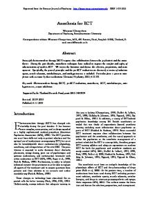
SIGGRAPH 2010 Course

Abstract Importance sampling provides a practical, production-proven method for integrating diﬀuse and glossy surface reflections with arbitrary image-based environment or area lighting constructs. Here, functions are evaluated at random points across a domain to produce an estimate of an integral. When using a large number of sample points, the method produces a very accurate result of the integral and provides a strong basis for simulating complex problems such as light transport. Frequently, using the necessary number of samples to reach the exact result is too computationally expensive and fewer samples are evaluated at the cost of visual noise, or variance, within the image. Importance sampling oﬀers a means to reduce the variance by skewing the samples toward regions of the illumination integral that provide the most energy. For instance, the direction of specular reflection or a bright light source within an environment more likely represent the final value of the integral than a random sample. The variance can be reduced more eﬃciently by combining multiple components of the illumination integral, such as the lighting and material function, to determine where to sample, which is the principle of Multiple Importance Sampling (MIS). As an alternative to the noise in importance sampling, Filtered Importance Sampling (FIS) can provide fast integration, where the lighting environment look-ups are prefiltered to give a smoother result with a significantly smaller number of samples. Importance sampling, MIS and FIS have various practical implications. In this quarter-day course, we cover the necessary background for using Monte Carlo-based techniques for direct lighting and explain how various visual eﬀects companies use these shading methods in their production pipelines.

Contents Course Overview

2

Biographies

3

1 Introduction 1.1 Overview of Course Material . . . . . . . . . . . . . . . . . . . . . . . .

4 5

2 Monte Carlo Methods 2.1 Estimators . . . . . . . . . . . . . . . . 2.2 Monte Carlo Integration . . . . . . . . 2.3 Variance Reduction Techniques . . . . 2.3.1 Importance Sampling . . . . . 2.3.2 Stratified Sampling . . . . . . . 2.3.3 Control variates . . . . . . . . 2.3.4 Defensive importance sampling 2.3.5 Multiple Importance Sampling

. . . . . . . .

. . . . . . . .

. . . . . . . .

. . . . . . . .

. . . . . . . .

. . . . . . . .

. . . . . . . .

. . . . . . . .

. . . . . . . .

. . . . . . . .

. . . . . . . .

. . . . . . . .

. . . . . . . .

. . . . . . . .

. . . . . . . .

. . . . . . . .

. . . . . . . .

. . . . . . . .

. . . . . . . .

3 Direct Illumination Formulation

5 5 7 8 9 10 10 11 11 12

4 Importance Sampling for Direct Illumination 4.1 BRDF-based Importance Sampling . . . . . . . . 4.1.1 Inverse Transform Sampling . . . . . . . . 4.1.2 Phong BRDF Sampling . . . . . . . . . . 4.1.3 Exponential Distribution Sampling . . . . 4.2 Image-Based Environment Importance Sampling 4.3 Quasi-Random Low-Discrepancy Sequences . . .

. . . . . .

. . . . . .

. . . . . .

. . . . . .

. . . . . .

. . . . . .

. . . . . .

. . . . . .

. . . . . .

. . . . . .

. . . . . .

. . . . . .

13 14 14 15 16 19 22

5 BRDF Proportional Filtered Importance Sampling 5.1 Foundation . . . . . . . . . . . . . . . . . . . . . . . 5.2 Environment Lights . . . . . . . . . . . . . . . . . . 5.3 Area Lights . . . . . . . . . . . . . . . . . . . . . . . 5.4 Analysis . . . . . . . . . . . . . . . . . . . . . . . . .

. . . .

. . . .

. . . .

. . . .

. . . .

. . . .

. . . .

. . . .

. . . .

. . . .

. . . .

22 23 24 27 29

. . . . . .

6 Multiple Importance Sampling 7 Practical Notes on Monte Carlo Sampling 7.1 Choosing Sampling Density . . . . . . . . . . . 7.2 Filtered Importance Sampling For Area Lights 7.3 What About Visibility? . . . . . . . . . . . . . 7.4 Resampled Importance Sampling . . . . . . . .

32 . . . .

. . . .

. . . .

. . . .

. . . .

. . . .

. . . .

. . . .

. . . .

. . . .

. . . .

. . . .

. . . .

. . . .

35 35 36 37 38

8 Importance Sampling Framework at MPC 8.1 Image Based Lighting Constraints . . . . . . . . . . . . . . . . . . . . . 8.1.1 Energy Conserving BRDFS and Albedo Pump-up . . . . . . . . 8.1.2 Dealing with Number of Samples . . . . . . . . . . . . . . . . . . 8.1.3 Raytracing Strategies in Clash of the Titans . . . . . . . . . . . . 8.2 Quick Implementation of Iridescence and Color Shifts with Filtered Importance Sampling . . . . . . . . . . . . . . . . . . . . . . . . . . . . . . 8.3 Sampling Strategies . . . . . . . . . . . . . . . . . . . . . . . . . . . . .

39 39 40 42 48

9 Conclusion

54

50 50

10 Acknowledgements

55

References

56

Course Overview Format: Quarter-Day (1.75 hr) Course Outline • Introduction (1 minute) Mark Colbert • Background (20 minutes) – Overview of the Illumination Integral and Monte Carlo Rendering – Importance Sampling – Phong BRDF Sampling – Exponential Distribution Sampling – Quasi-Random Low-Discrepancy Sequences • Filtered Importance Sampling (FIS) (15 minutes) – Motivation for a Smoother but Biased Estimator – BRDF Proportional Filtered Importance Sampling with Image-based Environment Lights ∗ MIP-map Filtering ∗ Ptex-based Cube Map Filtering – Analysis and Convergence • FIS for Area Lights in “A Christmas Carol” (10 minutes) – Decoupled Lighting Model – Ray Diﬀerentials – Filter Selection – Slide Map – Aliasing Artifacts – Real-time Interactive Setup for Lighters • Importance Sampling Framework at MPC (25 minutes) Guillaume Fran¸cois – Image-based Environment Importance Sampling – Image-based Lighting Constraints ∗ Energy Conserving BRDFs and Albedo Pump-up ∗ Dealing with Number of Samples ∗ Raytracing strategies in “Clash of the Titans” – Quick Implementation of Iridescence with Filtered Importance Sampling – Stochastic versus Quasi-Random Sequences • Multiple Importance Sampling (MIS) (30 minutes) Simon Premoˇze – Overview of MIS ∗ Mixture Sampling ∗ Control Variates ∗ Defensive Importance Sampling ∗ Mixture Sampling – Practical MIS ∗ Sampling Strategies ∗ Correlated Sampling – FIS and MIS • Questions (5 minutes) All Presenters

2

Biographies Mark Colbert Software Engineer Google [email protected] http://www.cs.ucf.edu/∼colbert Mark is a Software Engineer at Google working within on the Street View project. He was a Research and Development Engineer at ImageMovers Digital where he worked in the render development group writing shaders and pipeline tools. He was the lead developer for the real-time lighting pre-visualization tool chain. His film credits include A Christmas Carol and the upcoming movie Mars Needs Moms. In 2008, he graduated with a Ph.D. in Computer Science from the University Central Florida.

Simon Premoˇ ze simon ’DOT’ premoze ’AT’ gmail ’DOT’ com Simon Premoze received a B.S. in Computer Science from the University of Colorado at Boulder and was granted a Ph.D. in Computer Science from the University of Utah. He was a postdoctoral research associate at Columbia University where he worked on volume rendering and global illumination. He has been an R&D engineer at Industrial Light and Magic where he worked on a variety of rendering problems in production. His current research interests include global illumination and rendering algorithms, modeling natural phenomena and reflectance models. Previously he worked on computer simulation and visualization of liquid crystal phase transitions and dynamics of liquid crystals.

Guillaume Fran¸cois Shader Writer Weta Digital [email protected] Guillaume Francois was a Shader Writer at the Moving Picture Company where he is responsible for the Image Based Lighting shading pipeline. His interests and work also include atmospheric scattering, skin modeling and rendering and other rendering challenges. His film credits include G.I. Joe: The Rise of Cobra, Prince of Persia: The Sands of Time and Clash of the Titans. In 2008, he graduated with a Ph.D. in Computer Science from the University of Rennes I.

3

c �2009 ImageMovers Digital.

Figure 1: The broad glossy and diﬀuse reflections from an area light source were required to simulate the soft appearance of Belle in Disney’s A Christmas Carol. Here, filtered importance sampling was used to provide an eﬃcient and eﬀective result for the soft reflections.

1

Introduction

As the visual eﬀects and game industries strive for increasing realism, more complex lighting and material models are being tested and applied to achieve high fidelity images. As one approach, area and image-based lighting models are being combined with diﬀuse and glossy surface models to provide rich reflection detail (Figure 1). Unfortunately, the computation time required for brute force integration of these models is rather expensive. The cost can have a strong impact on the eﬀectiveness and benefit of complex lighting models in a production pipeline. For visual eﬀects, this implies the iteration time expands as the render times increase for an artist tweaking the appearance of a synthesized image. For games, the large computation may drop game performance below an acceptable level preventing the use of the model all together. Importance sampling provides a means to reduce the cost of brute force integration by selectively evaluating elements of the integrand based on prior knowledge, i.e. an educated guess. However, determining the prior knowledge is tricky since the illumination integral contains the product of the incoming light and the material reflectance function. Methods such as Multiple Importance Sampling (MIS) provide a way to account for the various components and solve for the reflectance with a relatively small number of samples. Another method of reducing this computational burden is through Filtered Importance Sampling (FIS) [CK07, KC08]. Although the method was originally intended for GPU-based material design, the algorithm’s flexibility and simple parallelization makes it amenable for rendering directly illuminated glossy surfaces in a production context. To that end, the approach has been used in movies such as Iron Man 2, A Christmas Carol, Terminator 4, Clash of the Titans, and Percy Jackson and the Olympians: The Lightning Thief. The goal of this course is to provide the audience with the necessary nuts and bolts in theory and code to understand and implement an importance sampling-based shading system. To that end, the following is presented as a tutorial for the reader.

4

1.1

Overview of Course Material

In the following course notes, we discuss Monte Carlo (MC) numerical integration and how importance sampling can provide a computationally cheaper solution than brute force MC (Section 2). We overview the underlying theory and math for integrating area and image-based lighting environments with material reflectance models (Section 3) and apply the importance sampling theory to rendering (Section 4). In the process, the formula and code for material-based and image-based environment sampling will be derived as reference for the reader. Next, we explain how the importance sampling framework can be adapted to support filtering and demonstrate how to improve computational eﬃciency for area and imagebased environment lighting with FIS (Section 5). We also provide empirical analysis on the various artifacts associated with FIS. We discuss other means to reduce the cost associated with importance sampling by using a technique called Multiple Importance Sampling (Section 6). Last, practical notes are provided for implementing importance sampling in a production pipeline (Section 7). This includes describing some solutions and tricks to eﬃciently render large and complex scenes when using the techniques presented in this course (Section 8).

2

Monte Carlo Methods

The term Monte Carlo refers to all methods that use a statistical sampling processes to approximate solutions to quantitative problems. It can be used for a wide variety of probabilistic problems ranging from numerical integration to optimization. These methods are used in many application domains such as economics, robotics and nuclear engineering. In this section, we describe some basic concepts of Monte Carlo integration. After a brief overview of the Monte Carlo methods, we introduce the principle of Monte Carlo integration and look at some of the basic statistical properties. Then, we describe some basic variance reduction techniques, such as importance sampling, control variates, and mixture sampling, that we use in later sections in the context of light transport. This section is only a brief summary, but it does provide some insights and intuition about why some methods perform better than other and describes the circumstances one should use a particular method. We encourage interested readers to learn more about Monte Carlo methods and probability in many excellent books [KW86, SG69, HH64] and papers that exist on the topic. Readers who are mostly interested in the practical implementation Monte Carlo methods for rendering can skip this section.

2.1

Estimators

A continuous random variable X is a quantity that randomly takes on a value x that lies on the real line (−∞, ∞). The values of x can be quantitatively described by the probability density function (PDF) p. The probability that x will take a value on some interval between a and b is then � b P r{a ≤ X ≤ b} = p(x)dx. (1) a

The probability density function p(x) must satisfy two conditions: 1. It is always positive: p(x) ≥ 0

5

2. It is normalized:

�

∞

p(x)dx = 1

−∞

It is important to understand the diﬀerence between probability and the probability density function. The probability, or likelihood, of an event takes values strictly between 0 (impossible event, it never happens) and 1 (certain event, it always occurs). On the other hand, the probability density function describes the relative likelihood of a random variable (or event) having a certain value. For instance, if p(x1 ) = 10 and p(x2 ) = 100, then the random variable with the PDF p is ten times more likely to have a value near x1 than near x2 . The relationship between the probability density function p and the probability P r is defined in Equation (1). Other important concepts to understand are expected value and variance of a random variable. The expectation (or expected value) of a random variable Y = f (X) is � E[Y ] = f (x)p(x)dx (2) Ω

and its variance is

V [Y ] = E[(Y − E[Y ])2 ].

(3)

Intuitively, expected value (or mean value) is just the average value of the random variable. Note that expected value should not be confused with the most probable value. On the other hand, variance measures how much the values of some random variable deviate from its mean or expected value. The higher the variance, the more values diﬀer from the average value. The expected value has a few useful properties: 1. The expected value of the sum of two random variables X and Y is the sum of the expected values of those variables: E[X + Y ] = E[X] + E[Y ] Since functions of random variables are also random variables, this principle applies to the sum of functions of random variables: E[f (X) + g(Y )] = E[f (X)] + E[g(Y )] The above holds true even if variables X and Y are correlated. 2. For any constant a, the expected value and variance for aX are E[aY ]

= aE[Y ]

V [aY ]

= a2 V [Y ]

If we want to compute an approximation to some unknown quantity Q (i.e.the estimand or quantity of interest), a function F of random variables X1 , . . . , XN is called an estimator if its mean (expected value) E[F ] is a usable approximation to Q: FN = FN (X1 , . . . , XN )

(4)

A particular numerical value of FN is called an estimate. Q can be any function that we might be interested in. In rendering, Q can be the amount of light that reaches a point on a surface or the amount of light reflected from the surface. There are many possible estimators. In general, we want Monte Carlo estimators to provide good estimates as fast as possible. How do we choose a good estimator? First, we need to establish some criteria for what good means by looking at the properties of Monte Carlo estimators:

6

• Error error = FN − Q

Mean Square Error (MSE) of an estimator F is then MSE = E[(FN − Q)2 ]

(5)

β[FN ] = E[FN − Q]

(6)

• Bias Bias β is the expected value of the error:

The estimator is unbiased if β[FN ] = 0 for sample size N : E[FN ] = Q

for allN ≥ 1.

(7)

An obvious advantage of the unbiased estimator is that we are guaranteed to get the correct value of quantity of interest Q if enough samples are taken. Furthermore, the expected value of an unbiased estimator will be the correct value after any number of samples. The mean square error of the estimator can be also written as (8) MSE[FN ] = V [FN ] + β[FN ]2 . For unbiased estimators, the MSE is the same as the variance. For biased estimators, the error is much more diﬃcult to estimate. It is also important to know that a biased estimator may not give a correct estimate for Q even if an infinite number of samples are taken. In practice, a biased estimator may have some desirable properties, such as lower variance, which makes it very appealing for use in computer graphics. For example, in rendering, noise is a manifestation of variance. While taking more samples reduces the amount of noise, rendering using a biased estimator may have less noise for the same number of samples albeit producing diﬀerent images. • Consistency An estimator is consistent if the error goes to zero as the number of samples grows: P r{ lim FN = Q} = 1. N →∞

(9)

The above equation is essentially saying that if we use a consistent estimator, we are one hundred percent certain that the answer is correct if we increase the number of samples. Consistency is a stronger condition than requiring the estimator to be unbiased. It is still possible that an unbiased estimator is not consistent, in which case its variance is infinite. A biased estimator is consistent if its bias β decreases to 0 as the number of samples N increases.

2.2

Monte Carlo Integration

The basic idea behind Monte Carlo integration is evaluation of the integral � I= f (x)dx

(10)

Ω

using random sampling. Here, N random points X1 , X2 , . . . , XN are independently sampled from some density function p and used to approximate I, N 1 � f (Xi ). IˆN = N i=1

7

(11)

Notation note: A realization of an estimator F , namely FN , is the same as IˆN . The subscript N emphasizes that Iˆ is still a random variable and therefore its properties depend on how many samples were chosen. As N increases, the expected error of this estimate decreases. We want to choose N such that we have confidence that the estimate IˆN is good. The estimator IˆN is a crude but unbiased estimator for I and its variance is N 1 � 1 V [IˆN ] = V [ f (Xi )] = V [f (X)]. N i=1 N

(12)

From this variance estimate V [IˆN ] we can conclude the following: 1. The standard error of the estimator decreases with the square root of the sample size N . Recall that the standard error of IˆN is V [IˆN ]2 , so while the variance of √ the estimate is proportional to 1/N the standard deviation is proportional to 1/ N . Therefore, to reduce the error in half, we have to quadruple the number of samples. 2. The statistical error is independent of the dimensionality of the integral. This simply means that the computation does not increase exponentially when the dimensionality of the integral increases. So far, we have not made any assumptions about function f (x) we are trying to integrate. On the other hand, in the above discussion we have assumed that our random variable X is uniformly distributed over the integration domain Ω. Loosely speaking, a uniform distribution implies that the probability of choosing each sample is equal. Unfortunately, real problems are rarely this simple. For example, function f (x) can be zero in many regions and have very high values in other. If uniformly sampling the domain Ω, we may get very large variance. Also, sometimes it may not be possible to sample a space uniformly. In order to alleviate these problems, we can rewrite the estimator from Equation (11) as � I = f (x)dx �Ω f (x) = p(x)dx, Ω p(x) where p(x) is a probability density function in Ω. We can now generate N samples from distribution p(x) (instead of uniformly sampling Ω) to get N 1 � f (Xi ) Iˆp = . N i=1 p(Xi )

(13)

The simple Monte Carlo estimator was saw in Equation (11) is just a special case of the more general estimator in Equation (13) with p(x) being a uniform distribution in Ω. This estimator has the same variance properties we have seen above. One major advantage of Monte Carlo integration is that it is easy to understand and simple to use. If we can generate random samples using some density p(x) and (Xi ) have the ability to compute the sample weights, wi = fp(X , i = 1, . . . , N , then we can i) evaluate the integral. Monte Carlo methods are also flexible, robust and work well in higher dimensions where other numerical methods might fail.

2.3

Variance Reduction Techniques

One of the biggest disadvantages of Monte Carlo methods is a relatively slow convergence rate. As we have already discussed above, the root mean square (RMS) error converges

8

√ slowly at a rate of O(1/ N ), so we need to quadruple number of samples N to halve the error. Ideally, we would like to use an estimator which has both small variance and is computationally eﬃcient. Eﬃciency of a Monte Carlo estimator F is �[F ] =

1 V [F ]T [F ]

(14)

where V [F ] is the variance and T [F ] is the time needed to evaluate F . Therefore, the more eﬃcient the estimator is the lower the variance in a given (fixed) amount of time. One of the fundamental goals in researching Monte Carlo methods is to find or design eﬃcient estimators. These techniques are often called variance reduction techniques and include importance sampling, control variates, and adaptive sampling. We briefly review some of these techniques. In later sections, we apply these techniques to the direct illumination rendering problem.

2.3.1

Importance Sampling

Recall that a Monte Carlo estimator for some function f (x) over domain Ω is � f (x) I= p(x)dx Ω p(x) and the estimator is

N 1 � f (Xi ) Iˆp = . N i=1 p(Xi )

The variance of the estimator Iˆp depends on the density p(x) from which random samples are drawn. If we choose the density p(x) intelligently, the variance of the estimator is reduced. This is called importance sampling. p(x) is called the importance density and (Xi ) wi = fp(X is the importance weight. i) The best possible sampling density is p∗ (x) = cf (x) where c is proportionality constant 1 c= � . (15) f (x)dx Ω Here, the constant ensures that p∗ is normalized (i.e., it integrates to 1). The density p∗ (x) yields an estimator with zero variance. In practice, we cannot use this density, because we must know the value of the integral we want to compute to evaluate c. However, if we choose an importance density p(x) that has a similar shape to f (x), the variance can be reduced. It is also important to choose an importance density p such that it is simple and eﬃcient to evaluate. In practice, p can be designed by doing some of the following: 1. Discard or approximate some parts of f (x) such that function g(x) = f (x)p(x) can be integrated analytically. 2. Construct a low dimensional discrete approximation of f (x). 3. Approximate f (x) by using Taylor expansion. After g(x) is designed with any of the above methods, the density is then set to p(x) ∝ g(x). We show in next sections how to choose and compute densities in practice. Note: If the sampling density is not chosen carefully, the variance can be increased and can actually be infinite. Importance sampling is very eﬀective when function f (x) has large values on small portions of the domain. Another common problem that happens in importance sampling is when the sampling density has a similar shape to f (x) except

9

that f (x) has longer (wider) tails. In this case, the variance can become infinite. While importance sampling is a useful and powerful technique it should be used with care. Inappropriate importance density can result in poor estimates of the integral.

2.3.2

Stratified Sampling

If we partition integration domain Ω into a set of m disjoint subspaces Ω1 , . . . , Ωm (strata), we can evaluate the integral as a sum of integrals over the stratum Ωi . If we generate ni samples in each stratum (subspace Ωi ), the estimator becomes Iˆ =

ni m � 1 � f (Xi,k ) n i=1 i

(16)

k=1

whose variance is ˆ = V (I)

m � Vi i=1

ni

(17)

where Vi is the variance of f (x) in stratum Ωi . The expected error of this method, stratified sampling, is never higher than variance of ordinary unstratified sampling [Mit96]. However, stratified sampling is often better than importance sampling. The two methods can be combined to lower variance even further. Stratified sampling works well for low-dimensional integration, but it does not scale well for integrals of high dimensionality. The number of samples must also be chosen such that there is at least one sample drawn from each stratum.

2.3.3

Control variates

If we can rewrite the estimator as � � I= g(x)dx + (f (x) − g(x))dx Ω

(18)

Ω

where function g(x) can be analytically integrated and has the following property: V [f (x) − g(x)] ≤ V [f (x)]

(19)

then a new estimator is F =

�

Ω

g(x)dx +

N 1 � f (Xi ) − g(Xi ) . N i=1 p(Xi )

(20)

The variance of this new estimator will be lower than the original estimator. How do we decide whether to use importance sampling or control variates? Given function g(x) that is an approximation of f (x), then g(x) can be used either as an importance density or a control variate. If f (x) − g(x) is approximately uniform (constant), then using g(x) as a control variate is more eﬃcient. If f (x)/g(x) is approximately constant, then using importance sampling is more eﬃcient. Note that if g is proportional to p then the two estimators diﬀer only by a constant, and have therefore the same variance. If g is already used as the importance density, it would not be useful as a control variate, because the variance would not be reduced. Another criteria for choosing between importance sampling and control variates is whether g(x) can be integrated analytically (control variates may be preferable) or g can be sampled analytically (importance sampling).

10

2.3.4

Defensive importance sampling

We already mentioned in Section 2.3.1 that even if a sampling density p(x) has roughly the same shape as a target function f (x), but f (x) has longer tails, importance sampling will fail. When we draw a sample from the tails of p(x), the importance weight can be many times larger than weights in other parts of p(x). This causes high variance and in extreme cases the variance can be infinite. This deficiency can be address with defensive importance sampling [Hes95] which uses a defensive mixture distribution pα (x) instead of only the density p(x): pα (x) = αq(x) + (1 − α)p(x).

(21)

Here, 0 < α < 1 and q(x) is the target distribution. If we want to compute the integral � f (x)q(x)dx (22) I= Ω

where q(x) is the target density on the integration domain. The defensive mixture distribution pα (x) guarantees that the variance is bounded by 1/α times the variance of the uniform distribution estimator. It also bounds the importance weight to 1/α. However, oftentimes it may not be easy or possible to sample from the target density q(x). If q(x) can be decomposed into a product of several (simpler) densities, q(x) = q1 (x), . . . , qn (x) and each qi (x) can be easily sampled, then a more general mixture distribution of m densities can be used: m � pα = α0 p(x) + αj qj (x). (23) j=1

Here, the sum of all weights αj is one and each weight is greater than zero.

2.3.5

Multiple Importance Sampling

Many times we have to integrate a complex function whose target distribution has multiple modes (peaks or bright regions) and sampling with a single importance density may not capture all regions of the integrand. For example, this is a very common problem in rendering. If our scene contains diﬀuse and glossy surfaces illuminated by small and large area lights, we face a diﬃcult decision about what sampling strategy to use. For diﬀuse surfaces, one sampling strategy might be preferable to another. However, the opposite might be true for glossy surfaces. Suppose that we have n diﬀerent densities, p1 (x), . . . , pn (x), and generate ni samples for each pi (x). Now, we have many diﬀerent sampling strategies that work well in diﬀerent regions of the integrand, but are not good over the entire domain. The question is how to combine multiple strategies that minimize the overall variance without introducing bias. As a na¨ıve approach, one could average the sampling strategies. However, this will not produce optimal results [VG95]. Instead, we combine all n sampling strategies giving the estimator F =

ni n � 1 � f (Xi,j ) wi (Xi,j ) n p i i (Xi,j ) j=1 i=1

(24)

where weight wi , w1 , . . . , wn , provide weight for each sample drawn from some sampling strategy pi . All weights must be non-zero and the total sum must be 1 to ensure that the estimator remains unbiased. An obvious weighting function would be wi (x) = ci

11

pi (x) q(x)

(25)

where

q(x) = c1 p1 (x) + · · · + ck pk (x)

(26)

and all coeﬃcients ci are nonzero and sum to 1. In general, the best choice of weights turns out to be ni pi (x) wi (x) = � . k nk pk (x)

(27)

If we take exactly one sample, ni = 1 from each sampling density, the weight wi will be set according to current sampling strategy at x compared to the rest of the strategies: ni pi (x) wi (x) = � . k nk pk (x)

(28)

This weighting strategy is called the balance heuristic and is nearly optimal. It is possible to design better strategies for special cases, but universally the balance heuristic out performs most other stratigies. What is the diﬀerence between MIS and Defensive Importance Sampling? Multiple importance sampling (MIS) is optimal for a given set of sampling strategies. However, if we have chosen a bad or inadequate sampling strategy, MIS will not reduce variance. For example, if one of the strategies takes too many samples from low-valued regions and not enough from high-valued regions, the variance will increase. On the other hand, defensive importance sampling (DIS) can improve variance when a sampling strategy p is inadequate. When combined with a uniform density, DIS guarantees that the integrand will be sampled over entire domain. MIS with balance heuristic can be viewed as a special case of DIS (see Equation (21), and factor α coming from balance heuristic weights). We will show in later sections how to use MIS in practice and how to design sampling strategies for rendering.

3

Direct Illumination Formulation

The goal in direct illumination rendering is to compute for each shading point how much light from the surrounding environment is reflected toward the virtual camera (Figure 2). To convert the incoming light from one particular direction and position, Li (ωi , x), into reflected light toward the direction of the camera, ωo , we use the material function f , known as the Bidirectional Reflectance Distribution Function (BRDF). Common BRDFs are the the Lambert [Lam60] and Cook-Torrance [CT82] reflection models that resemble the diffuse and specular functions in Pixar’s RenderMan. To compute the total reflected light, Lo (ωo , x), the contributions from every incident direction ωi must be summed (or integrated, in the limit) over the hemisphere H, � Lo (ωo , x) = Li (ωi , x)f (ωo , ωi ) cos θi dωi . (29) Ω

This equation is referred to as the reflectance equation or the illumination integral. Here, θi is the angle between the surface normal and the incoming light direction ωi . In image-based lighting, the incoming light Li is approximated by an environment map, where each pixel corresponds to an incoming direction ωi and occlusion of the light can be computed using techniques such as ray tracing or shadow mapping. Even if ignoring occlusion, the numerical integration of Equation (29) for one shading point

12

Zo

Li

f Figure 2: Components of the Illumination Integral. Here, the incoming hemisphere of light rays are multiplied by the BRDF f and reflected towards the camera ωo at a given shading point. in the image requires thousands of pixels in the environment map to be multiplied with the BRDF and summed. Similarly when using an area light, the light’s surface can be discretized into many small elements. Each element is considered a point light source whose contribution is subtended by the orientation and distance of the element to the shading point. The elements’ emissions are attenuated by the BRDF and summed together to estimate the original area light’s reflection. In both cases, these operations are too computationally expensive for real-time rendering and often too slow for oﬄine rendering. Since we cannot aﬀord evaluating the illumination integral for all incident directions, we randomly choose a number of directions and evaluate the integrand, Li (ωi , x)f (ωo , wi) cos θi , at these directions to obtain samples of the integral. The average of these samples produces an estimate of the integral, which is the essence of Monte Carlo quadrature discussed in Section 2. If we had an infinite set of samples, the average of the samples would equal the true value of the integral. This is denoted as the expected value of the estimator. However, using only a practical, finite set of samples, the estimate varies from the actual solution and introduces noise, or variance, in the image. One way to reduce this noise is by choosing the most important samples that best approximate the integral.

4

Importance Sampling for Direct Illumination

Generating uniform random directions is not the best approach for approximating the illumination integral, Equation (29), if we have a rough idea about the behavior of the integrand. For instance, if we are reflecting an environment on a glossy material, it seems intuitively more eﬀective to sample directions around the specular direction (i.e. the mirror reflection direction), since much of the reflected light originates from these directions. As discussed in Section 2, we represent this mathematically using a probability density function (PDF) that defines the optimal directions for sampling. Recall, the PDF is a normalized function, where the integration over the entire domain of the function is equal to 1, and the peaks represent important regions for sampling. However, by skewing sample directions, not all estimates of the integral are equal and thus we must weigh them accordingly when averaging all the samples. For instance, one sample in the trough of the PDF is representative of what would be many samples if uniform sampling was used. Similarly, one sample around the peak of a PDF represents only a few samples with uniform sampling. To compensate for this property of the PDF-proportional sampling, we multiply each sample by the inverse of the PDF. This

13

S4 S3

1

S2

Uniform Distribution

S1

0

Figure 3: PDF proportional mapping. In this case, if a random number is chosen, where there exists an equal likelihood that any value between 0 and 1 will be produced, then more numbers will map to the important sample S2 and thus that direction will be sampled more often. yields a Monte Carlo estimator that uses the weighted average of all the samples, Lo (ωo , x) ≈ L�o (ωo , x) =

N 1 � Li (ωi , x)f (ωi , ωo ) cos θi . N i=1 p(ωi )

(30)

Defining an optimal PDF for the illumination integral requires an accurate approximation of the product between the material BRDF and the incident lighting. In practice, if the BRDF has higher frequencies than the environment, such as a glossy surface reflection with a blurry environment light source, the BRDF alone is suﬃcient to sample. Conversely, if the BRDF is low frequency, such as with diﬀuse reflection, then the environment is ideal to use for sampling. In the following sections, we will cover how to sample solely from the BRDF and solely from an image-based environment. Sampling from both distributions simultaneously is discussed in Section 2.3.5.

4.1

BRDF-based Importance Sampling

As one of the components of the illumination integral, the BRDF can provide a strong basis to guide the importance sampling for glossy surface reflection. While various ways exist to create uniformly random samples, such as pseudo-random or quasi-random numbers generators, we must convert the uniformly random values to be proportional or nearly proportional to the BRDF. Two BRDFs discussed and commonly used in production for glossy surface reflection include Phong’s reflectance model [Pho75] and the Cook-Torrance model [CT82] (similar to specular in Pixar’s RenderMan). Since the Cook-Torrance model is predominately driven by an exponential distribution, we will look at a general sampling strategy for this distribution. Here, we ignore other components of the reflectance model, such as the Fresnel term, since this can be handled using techniques such as multiple importance sampling (Section 2.3.5). The following provides a full derivation of these sampling formulas as reference for the reader.

4.1.1

Inverse Transform Sampling

As one method for warping the uniform distribution, we can convert the PDF into a Cumulative Distribution Function (CDF). Intuitively, think of a CDF as a mapping between a uniform distribution to a PDF-proportional distribution. In the discrete case, where there are only a finite number of samples, we can define the CDF by stacking each sample. For instance, if we divide all possible sampling directions for rendering into 4 discrete directions, where one of the sample directions, S2, is known a priori to be more important, then the probabilities of the 4 samples can be stacked together as depicted in Figure 3.

14

z Tv

v

Iv Figure 4: Illustration of the spherical coordinates (θv , φv ) for an arbitrary vector v. For continuous one-dimensional PDFs, we must map a uniform distribution of numbers to an infinite set of possible PDF proportional samples. This way, we can generate a random number from a uniform distribution and be more likely to obtain an important sample direction, just as more random values would map to the important sample S2. We can obtain the position of a sample Θ within the CDF by stacking all the previous samples before Θ on top of each other via integration, P (Θ) =

�

Θ

p(θ)dθ

(31)

0

To obtain the PDF-proportional sample from a random number, we set P (Θ) equal to a random value ξ and solve for Θ. In general, we denote the mapping from the random value to the sample direction distributed according to the PDF as P −1 (ξ).

4.1.2

Phong BRDF Sampling

In the Phong BRDF, the glossy reflection is modeled by a cosine falloﬀ centered around the specular reflection direction. We can represent the glossy component mathematically as cosn θs , where θs is the angle between the sample direction and the specular direction and n is the shininess of the surface, � Lo (ωo , x) = Li (ωi , x) cosn θs cos θi dωi . (32) Ω

To convert this material function into a PDF, we separate out the exponentiated cosine lobe from the illumination integral. The other components of the integrand are ignored for computational eﬃciency and mathematic simplicity. This results in a PDF that is in terms of the angles around the specular direction, p(θs , φs ). Here, θs and φs are the spherical coordinates of the sample direction in a coordinate frame where the specular direction is the z-axis (Figure 4). To formulate this PDF, we must first normalize the cosine lobe to integrate to one, cosn θs sin θs n+1 p(θs , φs ) = � 2π � π/2 = cosn θs sin θs . n θ sin θ dθ 2π cos s s s 0 0

(33)

The extra sine appears when converting to spherical coordinates from solid angles. Often times, this normalization term is also included in the BRDF to ensure the reflectance model is energy conserving.

15

Sample Directions. To generate the two-dimensional sample direction (θs , φs ) according to this PDF, it is best to find each dimension of the sample direction separately [PH04b]. Therefore, we need a PDF for each dimension so we can apply Equation (31) to convert the PDF into a CDF and create a partial sample direction. To accomplish this, the marginal probability of the θs direction, p(θs ), can be separated from p(θs , φs ) by integrating the PDF across the entire domain of φs , p(θs ) =

�

2π

p(θs , φs )dφs = (n + 1) cosn θs sin θs

(34)

0

This one-dimensional PDF can now be used to generate θs . Given the value of θs , we find the PDF for φs using the conditional probability p(φs |θs ) from Bayes’ theorem [Bis06] defined as, p(θs , φs ) 1 = . (35) p(φs |θs ) = p(θs ) 2π The two probability functions are converted into CDFs by Equation (31) and inverted to map a pair of independent uniform random variables (ξ1 , ξ2 ) to a sample direction (θs , φs ), � 1 � θs = arccos ξ1n+1 , (36) φs

=

2πξ2 .

(37)

Note that the integration for p(θs ) is actually,(1 − ξ1 )1/(n+1) , but because ξ1 is a uniformly distributed random variable between 0 and 1, (1−ξ1 ) is also uniformly distributed between 0 and 1. Moreover, this sampling strategy works for various other BRDFs such as the Lafortune reflectance model [LFTG97].

4.1.3

Exponential Distribution Sampling

Distributions driven by exponentials, including the Ward [War92] and Cook-Torrance [CT82] BRDF, cannot be analytically integrated like the Phong BRDF. Therefore, the inversion method will not work as presented in Section 4.1.2. As an alternative, we can use the Box-Muller transform [BM58] to sample the isotropic or anisotropic exponential distribution. The following provides an intuitive interpretation of the transform.

Formulation. In the two aforementioned BRDFs, the exponential distributions are

based around the halfway vector H between the incoming ωi and outgoing ωo direction, where H = (ωi + ωo )/ ||ωi + ωo ||. The BRDFs are then defined to be approximately proportional to � �� 2 sin2 φh cos φh + , (38) f (θh , φh ) ∝ exp − tan2 θh αx2 αy2 where θh and φh represent the zenith and azimuthal angle respectively (Figure 5) between the normal and the halfway vector and αx and αy are the roughness parameters, where αx = αy when the reflection is isotropic.

Sample Directions. We start by sampling φh uniformly, similar to the Phong BRDF,

φh = 2πξ2 .

16

(39)

Zo

n To

Th

H Zi

Ih Figure 5: Illustration of the halfway vector and the corresponding variables used for the exponential distributions. In the anisotropic case, this is insuﬃcient since the distribution is elliptical instead of circular. So, we scale the directions accordingly using the tangent and arc tangent, � � αy tan(2πξ2 ) . (40) φh = arctan αx However, using the arc tangent requires special care for each quadrant and thus expensive conditionals in the shader logic. As an alternative, we can look at the definition of the tangent, and get cos φh and sin φh directly, tan φh = sin φh = cos φh sin φh = cos φh =

�

�

αy tan(2πξ2 ) αx αy sin 2πξ2 αx cos 2πξ2 αy sin 2πξ2

(41) (42) (43)

αx2 cos2 2πξ2 + αy2 sin2 2πξ2 αx cos 2πξ2

αx2 cos2 2πξ2 + αy2 sin2 2πξ2

.

(44)

This eliminates any unnecessary conditional logic in the shader. Please note that the denominator is required to normalize the scaled values and ensure the cosine and sine are on the unit circle. Now that we have mapped the random value ξ2 to φh , we need to find a mapping of ξ1 to θh . Assuming we want to sample all values of the distribution, i.e. sample the range of f (θh , φh ), we can set the equation equal to the uniformly random variable ξ1 and solve for θh , � �� 2 sin2 φh cos φh 2 + (45) ξ1 = exp − tan θh αx2 αy2 � 2 � cos φh sin2 φh − log ξ1 = tan2 θh + (46) αx2 αy2 � � − log ξ1 θh = arctan � . (47) � sin2 φh � cos2 φh + αx2 αy2

However, this only lets us know the position of the halfway vector. To determine the incoming light direction to use for sampling, we can convert θh and φh into a Cartesian

17

coordinate representation of the halfway vector H and find ωi using, ωi = 2(ωo · H)H − ωo .

(48)

PDF Value. Given the sample direction ωi , we still must evaluate Equation (30) with a PDF value. As shown in [Wal05], this requires that the probability density of the two-dimensional Gaussian sampling must be warped into the space of the illumination integral. This warping operation can be done with using the Jacobian of the of the mapping. The basic idea is that given two two-dimensional PDFs, pa and pb , where the ith dimension of pa can be mapped from pb using the function ai and the measure of probability from a region B in pb is equal to a the mapped region of AB in pa , � � pa (a1 , a2 )da1 da2 = pb (b1 , b2 )db1 db2 , (49) AB

B

then the integrals can be related using the change of variables theorem from calculus. Here, the determinate of the Jacobian is used to convert the the variables, � � � � � ∂a1 ∂a2 ∂a2 ∂a1 �� − db1 db2 . (50) pa (a1 , a2 )da1 da2 = pa (a1 (b1 , b2 ), a2 (b1 , b2 )) � ∂b1 ∂b2 ∂b1 ∂b2 � AB B In the case of the exponential distribution, we must first transform from the sample space to the halfway vector angles that are generated, giving � � � ∂ξ1 ∂ξ2 ∂ξ2 ∂ξ1 �� 1 � p(H) = � − , ∂θh ∂φh ∂θh ∂φh � sin θh

where the sin θ compensates for the conversion between the spherical coordinate and solid angle space. This equation evaluates and simplifies to the the following PDF, � � �� 2 �� cos φh sin2 φh −2 sin θh � exp − tan2 θ cos2 φh + sin2 φh � + 2 2 3 h � � αx αy cos θh αx α �, � � 1y p(H) = �� αx αy · 2π(α2 cos2 φh +α2 sin2 φh ) −0 � � y x sin θh �� 2 �� sin2 φh 1 αy cos2 φh + αx sin2 φh �� cos φh � 2 + p(H) = � exp − tan θh �, � αx2 αy2 παx αy cos3 θh αy2 cos2 φh + αx2 sin2 φh � (51) � � 2 �� 2 1 cos φ sin φ h h p(H) = exp − tan2 θh + . παx αy cos3 θh αx2 αy2 Last, we multiply the Jacobian from the transformation from the halfway vector space to the sample direction space in Equation (48), p(ωi ) =

p(H) . 4(H · ωi )

(52)

Combining Equation (51) and Equation (52), we obtain the final PDF for the anisotropic distribution for use in the illumination integral approximation, � � 2 �� 1 cos φh sin2 φh 2 p(ωi ) = exp − tan θh + . (53) 4παx αy cos3 θh (H · ωi ) αx2 αy2

18

4.2

Image-Based Environment Importance Sampling

As an alternative to BRDF sampling, we can also use an image-based environment to direct illumination integration. Various methods have been researched for eﬃciently integrating reflections from image-based environment light sources, such as the Voronoi cell-based approach in [ARBJ03], median-cut method presented in [Deb05], and the Penrose tiling-based approach in [ODJ04]. In the theme of this course and for code simplicity, we will provide an importance sampling treatment of image-based environment sampling, as presented by [PH04a]. Here, the sampling will be similar to the approach presented in Section 4.1.2 for the Phong BRDF sampling.

Image to PDF Conversion. The underlying idea in importance sampling the

environment is to treat the image as a PDF. Sometimes this discrete version of a PDF is referred to as a Probability Mass Function (PMF). The PDF requires a mapping from the texture space of an image (u, v) to the spherical coordinate space (θ, φ). For programmatic simplicity, a latitude-longitude map provides a good choice where the texture coordinates are defined by linearly scaling the spherical coordinates, θ

2π u w π v. h

=

φ =

(54)

Here, w and h are the width and height in pixels of the texture space. Since we used an image where u is equally spaced with respect to v, there is a large warping around the poles of the spherical map. This results from the radius diminishing around the azimuth angle at a rate of sin θ. When building the PDF, we compensate for this warping by attenuating the PDF by sin θ. Environment images are often in color and the PDF is a scalar function of density. Thus, we need another mapping between the color of a texture element to a density value. A popular choice is to use the luminance value of the element, defined by, L(u, v) = 0.2126R(u, v) + 0.7152G(u, v) + 0.0722B(u, v).

(55)

The luminance value represents a perceptually-based metric for how various color intensities are perceived by the human visual system [CIE31]. The basic idea behind using this mapping for the density is that by assigning a higher probability of sampling to the values with higher perceived intensity, the result will visually converge faster than using an arbitrary metric. Putting it all together, we have a PDF for the texture element (u, v) defined as, p(u, v) ∝ L(u, v) sin θ. (56) Please note that the PDF is proportional and not equal to the right hand side since this currently represents an unnormalized function.

Marginal and Conditional CDFs. Given the PDF of the environment, we can now build the marginal and conditional CDFs as to sample the environment with two independent and uniformly distributed random variables (ξ1 , ξ2 ). The conditional CDFs are constructed by summing the PDF values for each column u, P (v|u) ∝

v � i=1

19

p(u, i).

(57)

The marginal CDF is then computed by summing the maximum conditional values for each column u, u � P (u) ∝ P (h|i). (58) i=1

Please note, this is not how conditional and marginal distributions are typically represented. Instead, these equations reflect how the CDF is computed in code. The CDFs are stored unnormalized to maximize numerical precision. This is addressed explicitly in the final sampling operation. Given a color image in latitude-longitude space, the following C++ code snippet produces the associated CDFs, given an image in the variable m_pData and the width, height, and the number of channels are defined respectively as m_width , m_height, and m_channels. unsigned int k=0; float angleFrac = M_PI / float(m_height); float theta = angleFrac * 0.5f; float sinTheta = 0.f; float *pSinTheta = (float*) alloca(sizeof(float)*m_height); for (unsigned int i=0; i < m_height; i++, theta += angleFrac) { pSinTheta[i] = sin(theta); } // convert the data into a marginal CDF along the columns float *pBuffer = malloc(m_width*(m_height+1)*sizeof(float)); float *pUDist = &pBuffer[m_width*m_height]; for (unsigned int i=0,m=0; i < m_width; i++, m+=m_height) { float *pVDist = &pBuffer[m]; k = i*m_channels; pVDist[0] = 0.2126f * m_pData[k+0] + 0.7152f * m_pData[k+1] + 0.0722f * m_pData[k+2]; pVDist[0] *= pSinTheta[0]; for (unsigned int j=1,k=(m_width+i)*m_channels; j < m_height; j++, k+=m_width*m_channels) { float lum = 0.2126f * m_pData[k+0] + 0.7152f * m_pData[k+1] + 0.0722f * m_pData[k+2]; lum *= pSinTheta[j]; pVDist[j] = pVDist[j-1] + lum; } if (i == 0) { pUDist[i] = pVDist[m_height-1]; } else {

20

pUDist[i] = pUDist[i-1] + pVDist[m_height-1]; } } Using the marginal and conditional CDFs defined by pUDist and pVDists, random variables are proportionally mapped to sample positions in the texture space (u, v) using a binary search. The following snippet demonstrates how to sample the CDFs with the C++ STL binary search function lower_bound. Here, the random values are accessible in the vector m_samples. float maxUVal = pUDist[m_width-1]; for (unsigned int i=0; i < m_samples.size(); i++) { float* pUPos = std::lower_bound(pUDist, pUDist+m_width, m_samples[i][0] * maxUVal); int u = pUPos - pUDist; float* pVDist = &pVDists[m_height*u]; float* pVPos = std::lower_bound(pVDist, pVDist+m_height, m_samples[i][1] * pVDist[m_height-1]); int v = pVPos - pVDist; // store u,v into appropriate data structure }

Sample Space PDF. Last, given the sample position in texture space, we must

determine the PDF to evaluate the illumination integral in Equation (30). As in Section 4.1.3, we must convert from the texture space to the space of the illumination integral using the Jacobian of the mapping. Given the linear mapping in Equation (54), the Jacobian is simply, w·h . (59) 2π Since only the CDF is stored, the diﬀerence between the neighboring CDF values is used to compute the value of the PDF. Moreover, since the CDF is unnormalized, the PDF is divided by the last and largest value in the marginal and conditional CDF. float angleFrac = M_PI / float(m_height); float invPdfNorm = (2.f * float(M_PI*M_PI) ) / float(m_width*m_height); float* pVDist = &pVDists[m_height*u]; // compute the actual PDF pdfU = (u == 0)?(pUDist[0]):(pUDist[u]-pUDist[u-1]); pdfU /= pUDist[m_width-1]; pdfV = (v == 0)?(pVDist[0]):(pVDist[v]-pVDist[v-1]); pdfV /= pVDist[m_height-1]; float theta = angleFrac * 0.5 + angleFrac * y; float invPdf = invPdfNorm / ( pdfU * pdfV ) * sin( theta );

21

4.3

Quasi-Random Low-Discrepancy Sequences

The problem with generating uniformly random sample directions using pseudo-random numbers is that the directions are not well distributed, leading to poor accuracy of the estimator in Equation (30). We can improve the accuracy by replacing pseudo-random numbers with quasi-random low-discrepancy sequences that intrinsically guarantee welldistributed directions [Kel01]. One such sequence is known as the Hammersley sequence. A random pair (ξ1 , ξ2 ) in the two-dimensional Hammersley sequence with N values is defined as, � � i (ξ1 , ξ2 ) = , Φ2 (i) , (60) N where the radical inverse function, Φ2 (i) returns the number obtained by reflecting the digits of the binary representation of i around the decimal point as illustrated in the following table. 1 2 3 4

Binary 1 10 11 100

Inverse Binary 0.1 0.01 0.11 0.001

Value 0.5 0.25 0.75 0.125

As provided in [KK02], this can be coded by a simple bit swapping operator in C. double HammersleyRadicalInverse(unsigned int bits) { bits = ( bits << 16 ) | (bits >> 16); bits = ((bits & 0x00FF00FF) << 8 ) | ((bits & 0xFF00FF00) bits = ((bits & 0x0F0F0F0F) << 4 ) | ((bits & 0xF0F0F0F0) bits = ((bits & 0x33333333) << 2 ) | ((bits & 0xCCCCCCCC) bits = ((bits & 0x55555555) << 1 ) | ((bits & 0xAAAAAAAA)

>> >> >> >>

8 4 2 1

); ); ); );

return (double) bits / (double) 0x100000000LL; } Another advantage of using low-discrepancy sequences is that we can reuse them for each pixel. The deterministic sequence ensures that no matter how many times the frame is rendered, the result will always be the same. Moreover, this makes the algorithm amenable for GPU rendering since we can pre-compute the low-discrepancy sequence and transfer them to the GPU using a constant buﬀer. Unfortunately, the deterministic sample sequences will turn noise into replicated specular reflections, or alias (Figure 6(a)). However, the aliasing can be suppressed using filtered importance sampling as explained in Section 5.

5

BRDF Proportional Filtered Importance Sampling

While importance sampling and low discrepancy sequences reduce the variance of the illumination integral, a large number of samples are still required to produce a smooth solution. If using a deterministic sampling sequence, the noise will appear as aliasing when performing BRDF proportional sampling. To remove the alias in the signal, we borrow from a standard method in signal processing and pre-filter the incoming signal (Figure 6(c)). However, to determine the support, or size, of the filter we need a computationally eﬃcient function capable of estimating the filtered region without over-filtering and dulling the reflectance or under-filtering and leaving the alias.

22

(a)

(b)

(c)

Figure 6: Deterministic importance sampling for every pixel causes an aliasing eﬀect in the illumination integral estimate (a). Typically, random samples are used for each pixel providing a noisier, but more visually acceptable result (b). With filtered importance sampling, we can use computationally eﬃcient, deterministic sampling while obtaining smooth results (c).

5.1

Foundation

If the PDF of a sample direction is small (that is to say, if the sample is not very probable), then it is quite unlikely that other samples will be generated in a similar direction. In such a case, we want the sample to bring illumination from the environment filtered over a large area, thereby providing a better approximation of the overall integration. On the other hand, if the PDF of a direction is high, other samples are likely to be generated in similar directions, thus multiple samples will help average out the error in the integration estimation from this region. In this case, the sample should only average a small area of the environment. We define this relationship in terms of the solid angle associated with a sample Ωs , computed as the inverse of the product between the PDF and the total number of samples, N , 1 Ωs = . (61) N · p(ωi , ωo )

However, this only provides a scalar solid angle and not the shape of the filter region. As an approximation, we assume that the filter region is circular around the incoming light direction ωi , i.e. the filter is isotropic. This approximation may cause some samples to gather light from inappropriate regions and thus over-filter the sample. However, the isotropy is simple and fast to compute as seen in the following sections. Moreover, any over-filtering can be easily addressed by adding more samples. For a theoretical foundation for this relationship and filter approximation, we refer the reader to [KC08]. Given Equation (61) and the BRDF importance sampling strategies discussed in Section 4.1, we must determine how to filter the various light sources. Eﬀectively, we must determine a function that maps Ωs to an area on a light source that can be eﬃciently filtered. The following sections define this mapping for two illumination models, imagebased environment and area light sources.

23

Figure 7: A visualization of a MIP-mapped environment texture, where Ωs /Ωp is shown on the 0th level of the environment map and the corresponding filtered sample is highlighted on level l.

5.2

Environment Lights

MIP-Map Filtering. When pre-filtering with environment lights, we should filter all pixels of the map within the solid angle Ωs from Equation (61) around the sample direction. To make the filtering eﬃcient, we use the MIP-map data structure [Wil83] commonly used for anti-aliasing textures. A MIP-map is a pyramidal set of images, where each pixel of level l is the filtered result of the four corresponding pixels of level l − 1 (Figure 7) and level zero is the original texture. Therefore, filtering all the pixels within the solid angle Ωs can be approximated by choosing an appropriate level of the MIP-map. First, we compute the number of environment map pixels in Ωs . Assuming the shape is isotropic (or circular), this is given by the ratio of Ωs to the solid angle subtended by one pixel of the 0th MIP-map level, Ωp . This, in turn, is given by the texture resolution, w · h, and the mapping distortion factor d(ωi ), Ωp =

d(ωi ) . w·h

(62)

The distortion factor corresponds to the size of a mapping in a certain direction ωi . This term compensates for the stretching at the poles in a latitude-longitude map or the outer edges of a dual paraboloid map. However, the distortion may be complex to derive and compute. In practice, we found that equally weighting each direction produces similar results to those obtained using correct distortion. As aforementioned, we want the environment map lookup to correspond to averaging Ωs /Ωp pixels, which yields the formula for the MIP-map level, � � � � � � 1 1 Ωs w·h 1 l = max , 0 = max log2 log2 − log2 (p(ωi , ωo )d(ωi )) , 0 . (63) 2 Ωp 2 N 2 For each sample direction, the filtering operation is reduced to evaluating Equation (63), and using l in the corresponding texture call. In NVIDIA’s GPU language Cg, l is fed to the function tex2Dlod() as the level of detail parameter when looking-up the environment map.

24

:s Ts

Zi

Figure 8: The parameters of the spherical cap used as the isotropic filter region for area lights.

Ptex Filtering of Cube Maps for RenderMan. In production renderers,

such as Pixar’s RenderMan, other intrinsic data structures can be used to achieve better filtering with less distortion than the proposed MIP-map filtering method. One option is the Per-face Texture (Ptex) environment representation [BL08]. Here, the Ptex format will store the environment as a cube map. This mapping provides relatively minimal distortion since the environment is projected onto each face of the cube, which is similar to GPU cube maps. However, unlike GPU cube maps, the Ptex algorithm will filter across the various faces of the cube map. This will provide a smooth, seamless transition when filtering a region present on multiple faces of the cube. In Pixar’s RenderMan, the filtered cube maps are accessed using the environment() function call. Here, the environment is passed four three-dimensional vectors representing the filter region. However, generating the filter region cannot be analytically computed as with the MIP-map level in the GPU approach. Instead, we generate a spherical cap (Figure 8), and orient the filter vectors around the cap. This once again represents our isotropic filter approximation. Here, we assume the filter region lies within a spherical cap with an area of Ωs and the entire cap is above the horizon. The bounds of the spherical cap with respect to the angle between the sample vector, θs , can be found by solving the equation for the area of a spherical cap, Ωs = 2π(1 − cos θs ), for θs giving, � � Ωs θs = arccos 1 − . (64) 2π The four vectors representing the filter region are then computed by rotating the sample direction by θs around two orthogonal directions (Figure 9). Given two orthogonal vectors, tV and bV, and the sample direction wi the filter region can be computed using the following RSL code snippet. float cosThetaCap = 1.0-1.0/(pdf * numSamples * 2.0 * PI); float sinThetaCap = sqrt( 1.0 - cosThetaCap*cosThetaCap ); vector cosThetaCapWi = cosThetaCap * wi; vector vector vector vector

wi_tp wi_tn wi_bp wi_bn

= = = =

cosThetaCapWi cosThetaCapWi cosThetaCapWi cosThetaCapWi

+ + -

sinThetaCap sinThetaCap sinThetaCap sinThetaCap

* * * *

tV; tV; bV; bV;

color filteredValue = environment( ptexEnvironmentMap, wi_tp, wi_bp, wi_tn, wi_bn,

25

Zi t

Zi,b+

Zi

t

Ts

b

t

Zi

Zi,t+

b

(a)

Ts

(b)

b (c)

Figure 9: Illustration of the rotation of ωi around the orthogonal vectors t and b to generate the filter region vectors or the ray diﬀerentials. "filter", "gaussian" ); Please note that the filter is forced to be Gaussian to prevent any sharpening artifacts from occurring by possible negative weight filters being set as the default in the renderer. Moreover, orthogonal vectors tV, bV and wi, i.e. the coordinate frame, must be smooth across the image. Since filtering is eﬀectively adding bias to the simulation, any large discontinuities in the coordinate frame will result in visual artifacts.

Smooth Coordinate Frame. When using the MIP-map based filtering, the coordinate frame is implicitly defined to be oriented in the texture space of the environment. When specifying the coordinate frame from an arbitrary sample vector, this requires more care to ensure the orientation vectors are continuous and smooth across the rendered image. To find these orthogonal vectors, denoted as t and b, we start with the guess vector bguess . Given this guess vector, we build a coordinate system using the orthogonality of the cross product operator, t = bguess × ωi

b=

ωi × t.

As bguess becomes parallel to ωi , a pole-like discontinuity artifact appears in the filtered reflectance. A common solution is to use another guess vector that is orthogonal to the degenerate case. This works well for stochastic sampling because the noise covers the flip. When using a large number of samples, the results will converge on the exact solution which will also mask the flip. Unfortunately, deterministic FIS introduces a bias and this flip appears as a tear in the reflection. Since ∂P ∂u and ∂P ∂v contain discontinuities between faces, the partial derivatives available in production renderers such as Pixar’s RenderMan are also ineligible to be the guess vector. Similarly, texture coordinate based diﬀerentials may have discontinuities depending on the layout of the UVs. The key here is to recognize the discontinuity always exists due to the underdetermined nature of the single vector coordinate system problem. Therefore, the goal is to hide the degenerate case from the camera. One approach is to anchor the coordinate system to the camera-visible geometry. This way, the surface curvature masks any artifacts due to a changing guess vector. As an indicator of this curvature, we can use the camera space normals n. However, the normals themselves do not make a good guess vector. Using n may result in a degenerate case when ωi is parallel to n. Alternatively, we choose the partial derivative of n with respect to the spherical direction φ. If we convert n to spherical coordinates such that n is equal to (cos φ sin θ, cos θ, sin φ sin θ) and find the vector with

26

Gn/GI (a)

Gn/GI (b)

Figure 10: The partial derivative of the normal in camera space, ∂n/∂φ, is taken (a) and stretched (b) to produce a guess vector for building coordinate frames that is smooth and anchored to the geometry and viewing direction. respect to ∂φ, we obtain the guess vector, (− sin φ sin θ, 0, cos φ sin θ). When using this guess vector with the reflection vector, a discontinuity commonly happens around the silhouette edge of the object. In order to eliminate the discontinuity, we stretch the guess directions such that the discontinuity occurs behind the silhouette edge. This is done by simply scaling and oﬀsetting θ and φ via θ� = θ/2+π/4 and φ� = 2(φ−π/2)+π/2. Using this method, we obtain a geometry-anchored, temporally smooth coordinate frame for isotropic surface reflection. Please note that this method would not work for anisotropic surfaces since the coordinate frame depends on the viewing direction.

5.3

Area Lights

Area lights represent a higher dimensional mapping problem than the environment lighting model. In this case, for each shading point, both the position and orientation of the light determine the filter region. Instead of trying to find an analytical mapping as with the environment lights, we opt for an approximate numerical solution similar to the computed filter region used for image-based environments.

Mapping. The goal here is to find the region on the light that corresponds to Ωs of

the BRDF sample from Equation (61). This can accurately be done by projecting the shape of the sample region onto the light’s plane. However, this projected shape can be computationally expensive to evaluate. As an approximation, we assume the filter is isotropic. With respect to the hemisphere of incoming light directions, the isotropic filter is a spherical cap centered in the sample direction and is entirely above the horizon (Figure 8).

Ray Diﬀerentials. As an algorithmically simple approach for projecting the spher-

ical cap, we borrow from the texture filtering methods in ray tracing and use ray diﬀerentials [Ige99]. Here, we send two rays alongside the sample ray to determine the filter region on the area light. These supplemental rays are called ray diﬀerentials. The ray diﬀerentials are rotated by θs from the sample’s orientation in a direction orthogonal to the original sample (Figure 9). In this case, the sample direction is the incoming light direction ωi and the ray diﬀerentials are ωi rotated by θs in the direction of the smooth orthogonal vectors discussed in Section 5.2. We shoot the ray diﬀerentials and obtain

27

Zi

Zi

Zi

(a)

(b)

(c)

Figure 11: In determining the filter region of an area light sample, the sample ray and ray diﬀerentials intersect the plane of the area light (a). The intersecting area is used to build an isotropic filter region, i.e. an area light aligned box (b). The region is clipped by the bounds of the area light and used for filtering (c). a rectangle in the plane of the light which represents the filter region. To provide an isotropic filter response, the area of the filter region is computed and used to generate an area light-aligned box (Figure 11).

Filtering. The simple box filter can be computed by taking the ratio of the area

of the clipped filter region over the area of the light source. The clipping can become moderately complex to compute if the rectangle is not aligned with the area light coordinate system. To minimize the computation, the rectangle from the ray diﬀerentials is axis aligned thereby reducing the clipping operation to a series of min and max operations. However, this low quality filter produces noticeable artifacts that stem from the approximations made to compute the filter region. As a better filter and estimate of the projected elliptical shape of Ωs , we use a Gaussian filter kernel. Due to the axis aligned approximations made for fast clipping, we perform a relatively cheap integration of the filter region with the Gaussian kernel. For instance, if the filter region is translated such that the center of the clipped rectangle is at zero and if the clipped region is scaled by the width and height of the entire filter region, the problem can be formulated as, � +x � +y 1 exp(−x2 − y 2 )dxdy, (65) 2π −x −y where −x, +x, −y, and +y represent the scaled bounds of the clipped filter region. The function then has an analytical integral in terms of the error function erf , 1 (erf(−x) − erf(+x)) · (erf(−y) − erf(+y)). 4

(66)

Thus, the filtering convolution is reduced to four erf function calls, which has approximately the same computational complexity as four exp calls.

Slide Maps. Artists may also want to put a slide map, or gobo, in front of the light

source to add texture to the light color. Since the filter area with respect to the entire area light is known, the number of pixels is computed by scaling the ratio between the filter area and the area light size by the resolution of the slide map. The number of pixels are then converted into a MIP-map level using a formula similar to Equation (63) and the filtered texture value is accessed using the same method as described in Section 5.2.

28

0.7 0.6

5 Samples

50 Samples

RMS

50 Samples

0.5 0.4 0.3 0.2 0.1 0

200 Samples

Reference

50

100 Filtered Samples

150

200

(b) Phong, n=50

(a) Phong, n=50

Figure 12: On complex geometry, undersampling appears as blurring and dulling of the highlights although appearing visually acceptable around 50 samples (a). The blurring on complex geometry aﬀects the RMS (b) such that more samples are required to obtain an error similar to the spheres in Figure 14. However, due to the masking eﬀect of the high-frequency contours, the error is less noticeable than on smooth surfaces.

5.4

Analysis

Using the aforementioned methods, we can obtain accurate smooth glossy surface reflections with a relatively small number of samples. The following analyzes the resulting artifacts when using too few samples with area and image-based environment light sources. We discuss the convergence pattern associated with smooth and complex geometry on a few anecdotal cases.

Environment Lights. When viewing BRDF-based FIS integration with the en-

vironment light, undersampling causes a glossy material to appear duller (Figure 12). This is due to filter kernels not faithfully respecting the shape of the BRDF. This can cause seams to appear on smooth surfaces when using the GPU-based implementation. The seams occur from the image representation of the environment which has edge boundaries. When using with latitude-longitude environment parameterizations, the edge occurs along the left- and right-most regions of the maps. For the dual paraboloid parameterization, the artifacts occur when filtering in the transition region between the two hemispheres. In both cases, the seam artifacts appear since the reconstruction filter is performed in image space and not in a spherical environment space. [CK07] suggest using a scaled dual paraboloid environment parameterization to reduce this artifact. The scale results in a portion of the alternate side of each paraboloid to appear in the other’s map, which aﬀords limited filtering across hemisphere boundaries. However, this still produces a seam artifact if the scale is too small or when using too few samples. As mentioned in Section 5.2, the Ptex-based environment representation removes these artifacts by filtering across the boundary regions. In practice, if the reflector is rough due to displacement or a bump map, the latitude-longitude mapping can be suﬃcient since the seam will be masked by the surface variation.

Area Lights. Similar to environment lights, area lights also have an overall dulling when using too few samples. However, area lights do not have a seam associated with a

29

Area Light

Camera

(a) 16 samples

(b) 128 samples

(c) Top view of scene

Figure 13: Area light aliasing artifact. Here, the undersampling appears as ripples in the reflection (a) and can be reduced by sending more samples from the BRDF (b). filter boundary. Instead, the glossy area light reflections alias when only a small number of samples hit the emitter. This is evident when viewing reflecting surfaces that are perpendicular to the area light (Figure 13). The result is a low frequency, shimmering artifact that occurs until enough samples ray hit the light source. However, due to the low frequency property, the artifact tends to be masked by high frequency variations in the surface normal.

Convergence Rates. While these artifacts appear when using too few samples,

visually acceptable results typically appear around 40 to 60 samples. In Figure 14, the root mean squared (RMS) error is compared between BRDF-based filtered importance and regular environment map sampling. One measure of success for the method is to analyze the error with respect to the number of samples. This is called the convergence rate. As illustrated, FIS works well with glossy surfaces and respects the N 1/2 convergence rate associated with Monte Carlo quadrature. However, unlike standard Monte Carlo quadrature, the results are significantly smoother and require fewer samples for a visually pleasing solution. When comparing the results to deterministic environment map sampling, BRDFbased FIS performs better with glossy surfaces whereas environment sampling produces better matte reflections with a small number of samples. In practice, as the BRDF becomes more diﬀuse, the eﬀectiveness of BRDF-based FIS wanes as the artifacts become more prevalent. When looking at more complex geometry, such as the Buddha statue in Figure 12, we see a practical use case for FIS, where the only noticeable artifact is the dulling of the highlights. The high frequency contours of the surface cover up any seam artifacts and the results look visual pleasing around 50 samples per pixel. This method extends well for limited amount of anisotropic reflection, as seen in Figure 15. Unfortunately, as the amount of anisotropy increases the isotropic filter approximations become insuﬃcient. The result is the appearance of replicated specular reflections along the direction of high anisotropy. As an alternative, one can use anisotropic texture filtering. This is typically done by specifying the region of the filter instead of just controlling a blur or MIP-map parameter. However, this often does not provide good results. In practice, the sampling requires a small amount of over-filtering, or overlap on the filter region between samples. This property is intrinsically aﬀorded by the isotropic approximations. Care must be taken in order to perform this operation with an anisotropic

30

1.5

1.5 RMS

2

RMS

2

1

0.5

1

0.5

0

50 100 Env. Samples

150

200

10

100

1000

Spec. Exp.

0

50 100 Filtered. Samples

(a)

200

100

(b) Reference 10,000 Samples

Filtered Sampling Visualization

Filtered Sampling Error

Phong n = 17 100 Samples Phong n = 1000 200 Samples

(c) Figure 14: Comparison of filtered BRDF and environment importance sampling. Panel (a) shows the RMS error when rendering a sphere lit by the grace light probe. While both methods converge at a rate of N −1/2 , filtered BRDF importance sampling has a lower RMS overall, especially on more glossy materials. Visually, the BRDF importance sampling better captures many of the subtle features of the environment (b). Although the RMS figures suggest better performance for BRDF importance sampling, even for low-frequency glossy reflections with few samples, environment IS provides more visually pleasing images in such cases (c).

31

1000

Spec. Exp.

Phong n = 3 5 Samples

Environment Sampling Error

Environment Sampling Visualization

150

10

(a) Dx= 0.14, Dy= 0.01

Dx= 0.01 Dy= 0.01

Dx= 0.01 Dy= 0.08

Dx= 0.01 Dy= 0.29

(b)

(c)

(d)

Figure 15: The Ward anisotropic BRDF rendered using 40 filtered importance samples. The method works well on complex surfaces (a) as well as high frequency materials (b) with slightly anisotropic reflections (c). However, it breaks down when rendering more anisotropic materials (d) due to our approximate isotropic filter. filter and often the cost of anisotropic filtering outweighs the visual benefit. Instead, a few more isotropic samples will typically capture the reflection.

6

Multiple Importance Sampling

Recall that one of the main objectives in rendering is to approximate the illumination integral in Equation (29): � Lo (x, ωo ) = Li (x, ωi )f (ωo , ωi ) cos θi dωi Ω

which can be split into three components: incoming illumination Li , cosine weighted BRDF B and visibility function V . If we drop the spatial and angular, the illumination integral becomes � Lo =

Li BV dωi

(67)

Ω

and the traditional Monte Carlo estimator is

N � Li BV ˆo = 1 L N i=1 p(ωi )

(68)

where p(ωi ) is the importance sampling density. Ideally, the density function would be proportional to the product of LBV . Unfortunately, this is impossible for all but some artificially contrived scenes. We have to resort to some other density that will hopefully generate low variance in estimate. Let us examine a few possible options. When we have a diﬀuse BRDF and multiple area lights of diﬀerent sizes, we have two obvious choices for importance sampling densities. We can either sample according to the diﬀuse BRDF or lighting. Figure 16 illustrates the two scenarios. Using the diﬀuse BRDF, we sample the entire hemisphere, but only small portions of the hemisphere contain any lighting. So, many samples are completely wasted since the contribution will be zero. On the other hand, if we sample according to the lighting, none of the samples will be wasted because for any direction in which light is emitted the BRDF

32

Light

Light

ω �o

ht ig L

ht ig L

t gh Li

t gh Li

ω �o

Figure 16: Diﬀuse BRDF and area lights. When we have a diﬀuse BRDF and multiple area lights of diﬀerent sizes, two obvious sampling density choices are lighting (left) and BRDF (right). Note that BRDF sampling produces many samples that will be wasted, because there is no light emission in those directions. Sampling according to only the lighting produces lower variance. Light

t gh Li

ht ig L

ω �o

ht ig L

t gh Li

Light

ω �o

Figure 17: Glossy (specular) BRDF and area lights. Lighting (left) or BRDF (right) can be used as an importance sampling density. Note that light sampling produces many wasted samples because there will be no reflection in those directions. Sampling according to the BRDF provides better results. will reflect some light. For diﬀuse surfaces, it is better to sample according to lighting only. When we have glossy surfaces and many area lights, we can also sample according to the glossy BRDF or lighting densities. Figure 17 shows two sampling scenarios. In contrast to diﬀuse surfaces, glossy surfaces reflect light from a small solid angle. Using light sampling densities, most of the samples will be wasted because the surface will not reflect any light from those directions. Therefore, a better choice is to sample according to the glossy surface reflection, because there is a much larger chance that at least some sampled directions within a reflectance cone will have non-zero lighting contributions. When we have very glossy surfaces or diﬀuse only surfaces, the choice of sampling densities is fairly obvious. As highly glossy surfaces become duller (more diﬀuse) the choice becomes murkier and not straightforward. For slightly glossy surfaces, a combination of two sampling strategies should be used. So far, we have only looked at idealized situations where we have simple surfaces (composed of simple BRDFs) and no occluders. This is obviously an unrealistic situation. As shown in Figure 18 for a diﬀuse only surface, once we add occluders to the scene the sampling strategy becomes more complicated. Occluders can prevent light reaching the surface. Sampling according to lighting will generate proper directions, but lighting from those directions might be blocked. For the time being, we ignore visibility in our sampling density but we will return to it later and discuss what we could do to incorporate visibility into the sampling density. It is clear that complex lighting, surface properties, and occlusions cause the function

33

Light

ht ig L

t gh Li

Occluder

ω �o

Figure 18: Diﬀuse BRDF and area lights with occluder. While sampling according to lighting is still preferable, the occluder blocks many of the directions that contribute light. Ideally, we would not pick directions that are blocked by the occluder. Unfortunately, this cannot be easily achieved for arbitrary scenes and geometry. we want to approximate to be complex and discontinuous. This function can have many bright and dark regions and intensities can diﬀer by orders of magnitude. Since the function is very complex and does not have a nice formulation (due to occlusion) it is clear that either our sampling density will be complex or that we need more than one sampling density. Veach and Guibas [VG95] have demonstrated that by combining multiple sampling strategies, the variance can be reduced in situations where a single sampling strategy is bad (see Figure 19). How do we implement Multiple Importance Sampling? Given the two sampling strategies for lighting and BRDF discussed in Section 4, let p1 (x) and p2 (x) be a BRDF and light sampling density. The random variables X and Y are then X1,i ∼ p1 (x) f (X1,i ) Y1,i = p1 (X1,i )

X2,i ∼ p2 (x) Y2,i =

f (X2,i ) p2 (X2,i ) .

Now, we just need to combine the samples together: Yi = w1 Y1,i + w2 Y2,i .

(69)

The only remaining question is how to compute weights wi (x). We have already mentioned a few possible options in Section 2. One is using the balance heuristic, where the weights are: pi (x) (70) wi (x) = p1 (x) + p2 (x) and the final PDF p(x) for the combined sampling densities is: p(x) = w1 (x)p1 (x) + w2 (x)p2 (x).

(71)

Now, we have all the ingredients to implement multiple importance sampling. One of the remaining questions is how do we choose the number of samples for each sampling strategy. There are several possibilities: • Select a fixed number of samples for each strategy. For example, if N = 100, then N1 = 50 would be used for lighting sampling and N2 = 50 for BRDF sampling. Note that this is a relatively safe choice, although it could lead to suboptimal sample generation. If the BRDF is very glossy, some of the samples might be wasted, because too many samples are allocated for lighting sampling.

34

Glossiness

Radius

Sampling the light source

Sampling the surface

Sampling both the surface AND the light source

Figure 19: Combining many sampling strategies using Multiple Importance Sampling (MIS) produces superior results to using a single sampling density. Image from Veach and Guibas [VG95]. • Alternatively, the number of samples for each sampling strategy can be adjusted based on a heuristic, such as a combination of the solid angle of the light and glossiness of the surface. A reasonable strategy might be to have a minimum number of samples that will be taken according to each strategy and then distribute the rest based on the heuristic. For instance, if N = 100, we might allocate 20 samples to each sampling strategy. The remaining 60 samples would be distributed based on the glossiness of the surface and the light’s solid angle. Notes. Multiple importance sampling is an unbiased method for reducing the variance of Monte Carlo estimators. However, if it is used in conjunction with filtered importance sampling (e.g., filtered importance sampling is used to filter environment lighting) the method is biased due to the nature of FIS. For visual eﬀects applications, this is not troublesome as the noise can be greatly reduced. While MIS reduces the variance, there are still configurations where the variance will be high. As Kollig and Keller [KK00] pointed out, multiple importance sampling attempts to hide a weakness of using a single density function. If, however, only one sampling density exists for some region of our integration domain Ω, the multiple importance sampling will revert to a standard importance sampling. Kollig and Keller call this an insuﬃcient set of techniques [KK00]. We emphasize again, if inappropriate sampling densities are chosen, multiple importance sampling will not help to reduce the variance.

7 7.1

Practical Notes on Monte Carlo Sampling Choosing Sampling Density

The eﬀectiveness of importance sampling depends on the choice of the importance sampling density p(x). Figure 20 shows the diﬀerences between uniform and importance sampling. Figure 21 illustrates why the choice of importance sampling density is crucial for

35

Figure 20: (Left) A function f (x) can has many peaks. There might not be a single importance sampling density p(x) that can capture regions where the function f (x) has large values. (Middle) If samples (in red) are chosen uniformly, the variance will be high, because we oversample regions where the function is low (dark regions) and undersamples regions where the function is high (bright regions). (Right) If appropriate sampling density is used, we take many more samples (in green) in regions where the function has high values and thus reduce the variance. variance reduction. The examples in the figure demonstrate that inappropriate sampling density can increase variance, which can even become infinite. p(x)

f (x)

p(x)

f (x)

f (x)

Figure 21: Bad choice of importance sampling density. The sampling density does not match the shape of the function f (x) we want to evaluate. Only a small portion of the regions in the density function p(x) overlap (in orange) the non-zero parts of the function. A bad choice of importance sampling density will increase variance and not reduce it.

7.2

Filtered Importance Sampling For Area Lights

Previous sections have described in great detail how to apply filtered importance sampling for infinite (hemispherical) lights. A small extension could be used for filtered importance sampling for textured area lights. This is an alternative approximation to what was described Section 5.3. Recall that each sampled ray has a solid angle: Ωs =

1 . N p(θ, φ)

When the intersection with the sampled ray is found, we can approximate the area on the surface of the hit object by looking at the distance to the hit object and the solid angle of the ray: �xi − x�2 · Ωs A(xi ) ≈ . (72) cos θi For the above to hold true, we assume that the cross-sectional area is locally flat (Figure 22). Now that we have the estimated cross-section of the intersection A(xi ), we can estimate the mipmap level l based on this area: � � 1 A(xi ) 1 l = log2 = (log2 A(x1 ) − log2 Apixel ) (73) 2 Apixel 2

36

A(xi )

xi

ω �i

ω �o

x Figure 22: Cross-sectional footprint of ray intersection. where Apixel is the object space area covered by one pixel. It is used to convert areas from object space to texel space. We can use this formula to filter the texture on area lights when using multiple importance sampling. It is important to recognize that this is a crude approximation. When part of the ray footprint is outside the textured area, the light contribution will be underestimated and wrong. Still, this approximation gives plausible results.

7.3

What About Visibility?

We have seen in Section 2.3.5 that the idealMonte Carlo estimator should be N � Li BV ˆo = 1 L . N i=1 p(ω)

So far, we have been focusing on sampling from either the lighting, BRDF or a combination of sampling strategies using MIS. However, several recent sampling algorithms explicitly compute and sample an approximation of the product between the lighting and BRDF. Two-stage importance sampling [CETC06] and quadtree-based product sampling [CJAMJ05, CAM08b] hierarchically approximate a BRDF at a given point on the surface and combine it with the incoming light Li . Some of these methods can be fairly costly or may require precomputed data structures for BRDFs. If BRDFs are spatially varying, some of these methods may not be practical since they would require too much storage for all the BRDFs in the scene. We can take this further by adding visibility into the mix to lower the variance. Sampling from a triple product of lighting, BRDF and visibility, LBV , is diﬃcult at best. Exact visibility would take a long time to pre-compute and would be expensive to store. We can use an approximate visibility V¯ , thus making the estimator LB V¯ . The problem with this approach is that approximate visibility V¯ would have to be nonzero everywhere true visibility V is nonzero. This brings us back to the initial problem, because in order to guarantee this condition is satisfied we would have to compute visibility in all directions.

37

On the other hand, we can use the estimator LB V¯ as a control variate: � N � Li B V¯ − αLi B V¯ ˆo = 1 L + α Li B V¯ dωi . N i=1 p(ω)

(74)

Remember that a control variate requires the function f − g to be approximately constant. Even if visibility is crudely approximated, this condition can be satisfied. Clarberg and Akenine M¨ oller [CAM08a] analyze the variance for this case and describe an algorithm for using approximate visibility: • Create a compressed visibility cache using a compact bitwise representation stored at a sparse set of points in screen space. • Compute a rough estimate of Li B V¯ using the approximations. • Evaluate the diﬀerence between this approximation and the correct solution using Monte Carlo integration The reader is directed to [CAM08a] for detailed discussion and implementation notes.

7.4

Resampled Importance Sampling

Eﬃciency of a Monte Carlo estimator depends on the expense of the sample evaluation versus the cost of drawing a sample from better densities. For example, if function is cheap to compute, but finding the importance density is computationally expensive, there is probably an advantage to using a simpler sampling density with more samples. In rendering, casting visibility rays can be expensive and oftentimes we still want to avoid tracing too many shadow rays. Consider a situation where we have a glossy surface and we choose N samples based on the BRDF density. We also know that the surface is very glossy and therefore the cone around reflected lobe is fairly narrow. We might be able to use less than N visibility rays to approximate the light transport integral. We can do that by using resampled importance sampling [TCE05]. The idea is that from N partial estimates (BRDF times lighting, Li B) we only choose M values for which we will compute the visibility. More formally, resampled importance sampling is a generalization of importance sampling that permits unnormalized sampling densities or diﬃcult to sample densities (in our case, visibility) denoted as q. In rendering, the best density q would be q ∝ Li BV , but we can realistically at best only sample from another density p that is proportional to Li B. Instead of sampling from q, we generate a set of samples from a source distribution p and weight these samples appropriately. Then, we resample these samples by drawing a single sample from them with probability proportional to its weight. The basic algorithm proceeds as follows: • Choose a set of sample Xi from a known distribution p q(Xi ) • Associate a weight wi = p(X with each Xi , where q is the desired (possibly i) unknown distribution) • Generate the final samples Yi by sampling Xi with a distribution proportional to wi q(Xi ) If the weights wi are chosen to be wj = p(X then the resulting samples Yi will be i) approximately distributed to q. The processes of resampling is equivalent to filtering. In rendering applications, we use importance resampling as follows: • Generate N samples from some proposal distribution p(x). This is as before, where we created samples from either lighting density, BRDF density or combined MIS density.

38

• Compute the weights (e.g., luminance) of partial contributions (Li B, but no visibility yet). • Compute the discrete distribution from these weights. • Chose M samples from the above N samples. These samples are chosen based on the importance density that we computed in previous step. • Shoot shadow rays for these M samples, add computed visibility to each sample and apply proper weighting (based on the probability with which each sample was chosen). Note that although the desired target density q(x) is unknown a priori because of the visibility, we never sample from it. We only need to be able to evaluate it and that is straightforward as long as as we can evaluate visibility V . Resamples Importance Sampling (RIS) is better than importance sampling when: • q is a better importance sampling density than p. • Computing proposals is much cheaper than computing actual samples. RIS takes advantage of diﬀerences in the variance computation expense. More details and examples can be found in [TCE05].

8

Importance Sampling Framework at MPC

The Moving Picture Company recently developed a complete Image-Based Lighting solution in order to tackle the challenges of movies such as Clash of the Titans, Harry Potter and The Deathly Hallows and The Chronicles of Narnia: The voyage of the Dawn Treader. This project required us to render photorealistic creatures with highly reflective or wet surfaces, where fast and accurate specular and glossy reflections would be key to achieving the look. Alongside the creatures, we rendered a complete city environment, for which we would rely heavily on IBL for diﬀuse lighting. Rather than augmenting traditional lighting techniques, our IBL tools became the standard solution and replaced classical lighting techniques in the majority of shots. This required us to tackle many problems, such as ensuring energy conservation and making ray-tracing of incredibly heavy scenes eﬃcient by maximizing the bang for the buck of each ray traced. This section will cover some of these techniques and provide practical use cases of importance sampling and filtered importance sampling at MPC.

8.1

Image Based Lighting Constraints

Image Based Lighting allows the user to easily represent lighting coming from an almost infinite number of directional light sources. Diﬀerent techniques can be used to compute the diﬀuse and specular contributions. Each of these techniques have diﬀerent advantages in term of accuracy of the lighting and occlusion estimations as well as advantages in terms of computational cost. Amongst these techniques, the MPC pipeline uses a classic Dome Light, Environment Map Blurring, Importance Sampling and Filtered Importance Sampling. This allows the artist to choose a method based on its accuracy in the lighting, occlusion estimation, speed or memory consumption. The use of Image Based Lighting raises diﬀerent practical problems. This section describe some of the findings we made when using importance sampling for production purposes. We found that one important aspect raised by the introduction of this lighting technique in the MPC rendering pipeline was the diﬃculty to accurately estimate the incident lighting and at the same time ensure the quality of the shadows. Section 8.1.3 describes the ray-tracing solutions we developed at MPC to account for the variety of cases that our lighters encountered on the project Clash of the Titans.

39

c Figure 23: Rendering of the Kraken character from Clash of The Titans. �Warner Bros Another aspect of IBL and Important Sampling is their ability to faithfully reproduce reflections. However, this functionality strongly depends on the choice of the BRDF. Section 4.1 presents how to sample the BRDF. In the next subsection, we describe one key aspect to account for in the choice of a BRDF when rendering feature films images.

8.1.1

Energy Conserving BRDFS and Albedo Pump-up

One important requirement of the Image Based Lighting at MPC was to ensure energy conservation in order to avoid or reduce “light leakage.” Here, light leakage represents a loss of energy at near-grazing viewing directions which causes surfaces to appear darker near silhouette edges. When directly using energy-conserving BRDFs to compute reflectance, artists find a light-leaking or mirror reflection behavior around the grazing angles that is not intuitively expected. In the following, we compare the responses for three diﬀerent BRDFs and their integration with Importance Sampling and Filtered Importance Sampling for computing the specular contribution of semi glossy surfaces. The Ward BRDF [War92] has the advantage that its PDF is proportional to the BRDF and can be calculated at little extra cost. FIS using the Ward BRDF can give clean results even for a low number of samples. However, a direct implementation suﬀers from severe edge darkening, as visible in Figure 24. The Ashikhmin-Shirley BRDF [AS00], a Phong-like anisotropic BRDF, also has an easily derivable PDF. However, as shown Figure 24, this BRDF also suﬀers from an edge darkening even though much less than the Ward BRDF. Edward et al. [EBJ+ 06] presented a mathematical framework for enforcing energy conservation in a BRDF by specifying halfway vector distributions in simple twodimensional domains. The Halfway-Vector Disk BRDF gives the best results in terms of energy conservation and faithfully reproduces the sharpening of reflections visible at grazing angles in real-world surfaces (Figure 24). However, this accuracy made the BRDF unsuitable for our needs. In production scenes, where traditional delta light sources are still used, the tendency of the reflection to be perfectly specular around grazing angles produced unattractive highlights. In the end, we chose to use the Ashikhmin-Shirley BRDF, modified with an in-

40

Figure 24: Comparison of the filtered importance sampling for the BRDF of Ward, AshikhminShirley BRDF and The Halfway Vector Disk BRDF. The grey spheres represent the response to a uniform grey environment. A sphere using an ideal energy conserving BRDF would not be visible; it would reflect all the light from the environment at each point of the sphere, so every point on the sphere would be the same color as the environment.

41

Roughness

cos(șo)

Figure 25: The inverse of the measured total reflectance is used to normalize our Ashikhmin-Shirley BRDF -here lowered in exposure by 2 for display purposes-. house albedo pump-up based on the findings of Neumann et al [NNSK99]. While not completely physically accurate, this reduced the edge darkening to the point of being visually imperceptible. The pump-up also let us keep the blurry reflections at grazing angles desired by the artistic direction. One simple approach to study and correct BRDF light leakage is to render a mirror ball within a constant white environment as presented in Figure 24. The albedo can be normalized by multiplying the BRDF by a normalization factor. This factor can be precomputed and stored in a texture, as the one in Figure 25. Here, the texture represents the inverse of total reflectance for every viewing angle and roughness value. The roughness is mapped from 0 to 1 to make the BRDFs interchangeable and the albedo pump-up is computed by f actor(ωo , roughness) = �

1 . f (ω , ω , roughness) cos θi dωi o i Ω

(75)

Unfortunately, the addition of this arbitrary pump-up creates filtering artifacts when using FIS. Appearing as a ghosting eﬀect, these artifacts are caused by filtering with an unmodified PDF. Experimental tests show that these are created by an overestimation of the filtering kernel around directions with a low PDF. At first, we attempted to manually map filtering values that we compared visually to the correct result. While this gave acceptable results, it required long and fastidious experiments that had to be repeated for each BRDF. We therefore modified Equation (63), replacing the PDF by pow(pdf, α). By ensuring that α < 1, we successfully reduced the filtering for samples with a low PDF while preserving the correct filtering for samples with a high probability.

8.1.2

Dealing with Number of Samples

The quality of an image rendered with important sampling highly depends on the number of samples used to estimate the illumination integral (Equation (29)). A large number of samples usually provides accurate and noise free results, but it quickly becomes computationally prohibitive in complex scenes required for production. Here, the number of samples represents the amount texture lookups. In the case of ray-traced occlusion and inter-reflections, the sample count also represents the number of traced rays. While Filtered Importance Sampling allows us to use fewer samples than classical important sampling, it can still lead to prohibitive computations and it remains impor-

42

Camera

Camera

Figure 26: The number of samples needed to accurately estimate the incident lighting depends on the broadness of the specular lobe. tant to try to use an optimal numbers of samples, especially in the case of ray-traced occlusion or inter-reflections.

Adjusting the Number of Samples. Depending on the shape of the BRDF

and on the environment lighting, the number of samples should be adjusted. When considering no occlusion and lighting with a low frequency environment map, a small number of samples can eﬃciently estimate the incident lighting. On the contrary, using a low number of samples when lighting an object with high frequency incident lighting results in noisy images. While the frequency of the environment lighting usually remains unknown, the number of samples needed to accurately estimate Equation (29) can also be related to the broadness of the BRDF lobe, as shown in Figure 26. Rendering mirror like reflections only require a few samples while rough surface reflections require a large number of samples. We mapped the number of samples to the shininess parameter of our BRDF to provide the artist with a simple but tweakable solution. For a given roughness value, we rendered a reflective sphere with a diﬀerent number of samples -ranging from 1 to 256-, as well as a reference sphere rendered with a large number of samples. The next step was to choose the sphere with the lowest number of samples that would eﬀectively match the reference. We repeated this process for various values of roughness ranging from 0 to 1. This allowed us to plot the minimum number of samples required for each roughness value. We then fit a spline to the data to smoothen the results. The spline is stored in a look up table to minimize the computation for each pixel. The roughness values of a character are often described by a texture map to allow rich specular variations over the model, such as wet/dry or more or less oily areas etc.. The interesting aspect of this mapping is that the sampling is automatically adapted to these roughness values. It significantly optimized the number of samples per pixel, especially if there are regions that are mirror like.

43

Figure 27: A given set of images is rendered with diﬀerent sample counts and compared with a reference image to visually determine the necessary number of samples. Figure 28 schematizes the increase of the number of samples with the increase of the material roughness. In most cases, when considering semi-glossy reflections without occlusion or inter-reflections, we found that values from 16 to 64 samples provided us with acceptable results in term of image quality and render time (red curve in Figure 28). For materials with strong roughnesses, which required high number of samples, a per material/scene tweaking was performed in order to optimize the render times.

Adjusting the Number of Ray-traced Rays. The computation of occlusion

and inter-reflections for each sampled direction may be needed to accurately estimate the illumination integral. However, we found that computing the occlusion for the mapped number of samples was often too expensive and in many cases unnecessary. Depending on the scene geometry and its organization, we wanted to be able to adjust the amount of ray-tracing done (green curve in Figure 28). We introduced a percentage value that allowed us to only trace a certain number of sample directions while using interpolated occlusion or inter-reflection values for non ray-traced sampled directions. There are multiple ways to interpolate the occlusion samples. A brute force technique is to directly interpolate the occlusion value for a given direction using the closest ray-traced directions. However finding these rays can be computationally expensive and can overcome the advantage of tracing fewer rays. Moreover, sorting the precomputed rays to accelerate the search can be time consuming and memory prohibitive and needs to be repeated for each shading point. A more eﬃcient method consists of projecting the occlusion function -estimated using the ray-traced sampled directions- into a hemispherical basis such as hemispherical harmonics [KG05] or hemispherical wavelets. An estimated occlusion value for the nonray-traced directions is then obtained by evaluating the projected function in a new direction. Such methods give good interpolations when using enough coeﬃcients which can, as a result, be time and memory consuming. As our main requirement was to save memory and ensure speed, we simplify the problem and choose to sort the rays by quadrants and average the occlusion values

44

Number of Samples

200

100 64

Roughness

1 Mirror

Diffuse

Common glossy materials Environment lookups Raytraced Rays

Figure 28: Schematic view of the mapping of the number of samples used at MPC. per quadrant. The new directions will inherit the occlusion value of their respective quadrant. The quadrants are chosen around the direction of perfect reflection ωr to ensure a good distribution of rays in all the quadrants (Figure 29). This can be seen as a simplistic basis written: B1 (ωi ) = B2 (ωi ) = B3 (ωi ) = B4 (ωi ) =

(α−1)(β−1) 4 (α+1)(β−1) −4 (α+1)(β+1) 4 (α−1)(β+1) −4

with α = sign(ωi .T ), β = sign(ωi .B), and B and T being random vectors constructed such that (B, T, ωr ) is an orthonormal basis. The occlusion value Occ(ωi ) of a given direction ωi is then eﬃciently estimated as follow: Occ(ωi ) = B1 (ωi ) ∗ Occ1 + B2 (ωi ) ∗ Occ2 + B3 (ωi ) ∗ Occ3 + B4 (ωi ) ∗ Occ4 .

(76)

Here, Occ1 , Occ2 , Occ3 and Occ4 are the respective average occlusion of each quadrant. Even though this is a coarse approximation of the correct ray-traced occlusion, it gave us convincing results with a very small memory foot print. Furthermore, the simplicity of the projection made it easy to implement and provided us with quick but acceptable estimates of the occlusion values. When using this method, small artifacts, such as light leaks, could be visible for broad specular lobes but did not significantly change the overall look of the images in the very complex scenes we had in Clash of the Titans.

45

B 3

4

1

2

T

Ȧr

Figure 29: Each direction is located in a quadrant around the direction of the mirror reflection ωr . Given an array of sample directions ωi [], and the direction of the mirror reflection ωr , the following code snippet shows how to quickly estimate the visibility of the untraced rays. vector randomVector = normalize(vector(random(),random(),random())); vector T = randomVector^wr ; vector B = wr^T; color visibilityQuadrant[4] = {0,0,0,0}; int nSampleQuadrant[4] = {0,0,0,0}; int inQuadrant[4] = {0,0,0,0}; //Raytraced samples for(int i=0; i
46

(a)

(b)

Figure 30: Images rendered with 64 samples for the environment lookups with (a) 100% of traced rays for occlusion and (b) 60%. visibilityQuadrant[j] /= nSampleQuadrant[j]; } //Non raytraced samples for(int i=nRaytracedSamples; i
47

8.1.3

Raytracing Strategies in Clash of the Titans

While FIS gives us good results and an acceptable render time when not computing the visibility term, these techniques became computationally and memory prohibitive when using ray-tracing to compute occlusion and inter-reflections. Even the interpolation technique in the previous section is insuﬃcient at reducing the computational footprint. This section describes common methods which make possible the use of important sampling and ray-tracing within a production environment. MPC has long favored Image-Based Lighting techniques over traditional point-source and convolved environment approaches for the superior complexity and richness of the resulting lighting. Clash of the Titans presented a unique challenge to MPCs lighting and shading team: a full 3D city-harbor environment being attacked by a 350feet-tall sea monster. The city environment consisted of thousands of individual buildings and props, totaling millions of polygons, while the Kraken itself was just as complex -dozens of subdivision surfaces represented by cages of over 7 million polygons-. All this had to be lit using Image Based Lighting and be reflected in the water surface of the bay, while the Kraken itself required complex glossy and specular self-reflections. Despite significant performance improvements in recent versions, ray-tracing in Pixar’s RenderMan is still an expensive operation. There are two ways to speed up the raytracing process: 1) shoot less rays, or 2) reduce the computation that results from each ray hit.

Filtered Importance Sampling with Occlusion Caching and Interpolation. As shown in the images below, Filtered Importance Sampling allowed us to

dramatically reduce the number of rays required to sample the environment map effectively. Rather than use a single Image Based light source to illuminate the scenes, the initial image was split into diﬀerent sectors to provide artists with full control over the lighting. In all, there were 6 individual IBL sources used to light the scenes. This required that we modify our shaders to cache the interpolated occlusion and importance sampling intermediaries for each sampled direction, such that the results could be re-used for each IBL source rather than tracing more rays. These results were also shared with reflection cards -simple textured polygonal objects hand-placed by lighters to add shot-specific reflections -which could be either occlusive or additive depending on the needs of the lighters-.

Radiance/Irradiance Caching. For several years, MPC has used radiance caching techniques similar to those described in [SRKG07] to avoid expensive shading computations for ray hits. Since we use RenderMan’s point-based color bleeding solution [Chr09] on everything we render, we already have suitable irradiance pointclouds to be read for shading of reflections. Although these did not contain specular reflections, for the vast majority of cases the diﬀerence was not noticeable. The use of Importance Sampling made ray-tracing for diﬀuse IBL of the city environment feasible, but it was still too slow to calculate on a per-frame basis. We could not bake the illumination into shared irradiance caches since the client required a unique lighting direction for every shot, and baking the entire city for every shot would be impractical. Thus, we wrote a tool to bake multiple key frames from the shots camera move, then stitch the resulting pointclouds together to create an irradiance pointcloud that covered the entire length of the shot. The shadows and specular reflections of the key light on the city were calculated in the beauty render (using FIS to limit the number of samples), so the environment lighting and color bleeding only needed to be rebaked relatively infrequently. Many shots were only baked once.

48

(a) infinite trace distance - 3 hours

(b) 60 meters - 32 minutes

Figure 31: The comparison of two renders with a diﬀerent trace distance shows that reducing the c trace distance does not significantly aﬀect the look of the final image. �Warner Bros.

2

1

Figure 32: In Clash of the Titans, separate ray traces are performed with respective trace sets and trace distances.

Trace Distance and Trace Sets. A common technique for accelerating ray trac-

ing is to limit the distance rays are traced for intersections before giving up and returning an unoccluded result. This is especially important for massive models, such as the city environment, since searching only a small part of the scene reduces that amount of cache thrashing. Here, the trashing is caused by reloading geometry that does not fit entirely in main memory. For the particular case of lighting the city however, we required shadowing from the cliﬀs that surrounded the city in order to get the correct lighting result (Figure 31). The solution was to do two separate ray traces, one short distance against the highresolution model for local inter-building occlusion, and one long distance against a very low-resolution proxy model of the cliﬀs for environmental shadowing (Figure 32). The importance sampled ray directions were shared between the two traces, and rays were not retraced for the cliﬀs if they were already occluded by the city.

Ray-tracing Proxy Objects. Even using when Filtered Importance Sampling

to limit the number of samples, ray-tracing occlusion and specular reflections on a 7˜ million polygon subdivision surface like the Kraken, presented in Figure 33, was still impractical. This was due to the computational cost and memory requirements. In order to make this feasible, we used a technique similar to that described in [TL04]. While subdivision surfaces were used for the beauty render, the traceable objects

49

were in fact the original poly cages without any subdivision, thus giving much better performance both in memory usage and render time. In order to avoid intersections where the subdivision surface and the poly cage overlapped, we attached a second copy of the vertex positions to the subdivision surface, changing the way RenderMan interpolated the data such that the shaders would know where the polygonal cage was for each subdivision surface shading point, and could trace rays from this surface. In instances where this still was not enough, we used the same technique but tracing against a low-poly representation of the Kraken (˜2 million polygons).

8.2 Quick Implementation of Iridescence and Color Shifts with Filtered Importance Sampling The iridescence is an optical phenomenon commonly visible on multi-layered materials such as pearls, butterflies or snake skin. It consists in light wave interferences and diﬀraction on multiple thin films. Diﬀerent approaches can be used to either accurately estimate such phenomenon or to imitate it in a simpler way. The equations governing the iridescence phenomenon are complex and are not directly adaptable to the FIS theory because the importance sampling of such a BRDF is not straightforward. This section presents a simple and experimental approach to quickly imitate iridescent reflections when using Filtered Importance Sampling. One key idea is to show the flexibility and simplicity of the FIS algorithm, even for reproducing complex phenomena such as iridescence (see Figure 34). The two important aspects of the iridescence phenomenon to take into account are the shifting of the BRDF lobes and the very remarkable change of color depending on the viewing angle and light incident angle.

Shifting BRDF Lobe. Iridescent materials commonly present oﬀ-specular reflec-

tions, such as retro reflection. The Lafortune BRDF [LFTG97] or the Halfway Vector Disk BRDF oﬀer a good, controllable solution to this particular problem. However, note that comparable results can be obtained by shifting the BRDF lobes for other reflectance models, such as Ashikhmin-Shirley or Ward.

Color Variation. In order to provide the artist with a simple and editable irides-

cence eﬀect, we chose to control the change of color using a user defined ramp of color such as the one presented in Figure 35. This color variation acts like a Fresnel term and multiply the environment contributions depending on the angle between the incident light direction and the normal, θi . The interesting aspect of this method is its adaptability to the filtering scheme presented in Section 5. Note that in this case the distortion factor is equal to 1 when considering a ramp defined in θi . However, the distortion needs to be taken into account when considering ramps defined in cos(θi ). One future extension of this method for imitating iridescence in FIS will be to take into account the anisotropic behavior of certain iridescent materials, such as snake scales, by considering color ramps defined in θi and φi .

8.3

Sampling Strategies

One of the most commonly used algorithm for generating quasi-random sequences is the Hammersley algorithm (presented in Section 3), which is used in the FIS technique. One property of this technique is that it always generates the same sequence of quasi-random numbers for the same set of input parameters and provides an optimal deterministic

50

Figure 33: Bros.

c Renderings of the Kraken creature within diﬀerent lighting environments. �Warner

51

Figure 34: Iridescence and Filtered Importance Sampling. The colored reflection of the main sphere is a combination of mirror reflection and our iridescent reflection. The sphere in the lower right is a chrome reflection.

și

Figure 35: Example of ramp defining the color variations of the iridescence eﬀect: the sphere in the lower right shows a chrome reflection, the colored reflection of the main sphere is entirely due to iridescence.

52

Camera

Precomputed Hammersley Sequence

Randomly Shifted Selection of N Samples Camera

(a)

(b)

Figure 36: (a) Top: A quasi-random number sequence tends to generate spatial aliasing. Bottom: This can be avoided by using randomization algorithms. (b) The sequence selection is randomly shifted to avoid banding artifacts. sequence. However, this deterministic behavior tends to produce spatial aliasing as explained by Figure 36. Reusing the same sequence of randomly distributed points to sample a function combined with a low number of samples, introduces a visual artifact known as banding or “chandelier eﬀect” as seen in Figure 37(c). As explained by Colbert et al. [CPK06], in the case of Filtered Importance Sampling, this artifact is avoided as by blurring the environment map for each sample. However, the FIS technique was originally developed in the context of a GPU pipeline. Here, reflection occlusion and inter-reflection using ray-tracing are not commonly taken into account in the rendering equation (see Figure 37(a)). On the contrary, in production environments we need to capture these eﬀects and the banding becomes a problem for which a solution is required. One method to avoid these artifacts consists of using randomization methods. These methods, such as the Cranley-Patterson rotations or Random Digit Scrambling, “randomize” quasi-random sequences while keeping their low-discrepancy properties. A more complete description and comparison of these methods is presented in [KK02]. We use a simpler, fast to implement, technique at MPC: we store a large number of pre-computed quasi-random numbers using the Hammersley algorithm and shift the sequence used per shading point by oﬀsetting the entry in the table by a random number. As visible in Figure 37(d), this method introduces some noise back in the frame. However, the results are considerably better than a purely random solution (Figure 37(b)) and avoid banding artifacts. Furthermore it is often better than other stochastic sampling strategies (nrooks,jittered, etc...) as it is still conserving the low discrepancy properties. An interesting aspect of our method is that one can balance between the banding and noise by controlling the amplitude of the random shifting. For a number of samples N , we found that using shifting amplitudes in between N/2 and N gave us an acceptable balance. Note that the randomization method at MPC is a field that we will test and research more in the future.

53

(a)

(b)

(c)

(d)

Figure 37: Comparison in between diﬀerent sampling strategies. 16 samples are used to sample the BRDF. (a) FIS and Hammersley sampling with no occlusion, (b) IS and N-rook sampling with ray traced occlusion, (c) FIS and Hammersley sampling with ray traced occlusion, (d) FIS and Hammersley shifted sampling with ray traced occlusion.

9

Conclusion

Importance sampling is an eﬀective framework for eﬃciently evaluating the illumination integral with only a limited amount of pre-computation. The approach provides a means to simulate light reflectance from a broad variety of materials with a relatively simple trade oﬀ between visual fidelity and the number of samples used in the computation. The Filtered Importance Sampling (FIS) extension provides a practical solution for production rendering of both oﬄine visual eﬀects and real-time visualization. However, the approach does not work well for all situations, such as diﬀuse reflections. We have discussed the appearance of the FIS artifacts, which allows users to identify and diagnose problems associated with undersampling. For other cases, such as glossy reflection integration, FIS can provide smooth, deterministic results with a relatively small number of samples. Multiple Importance Sampling (MIS) can further reduce the number of samples necessary for visually acceptable results since both the lighting and material functions guide the integration evaluation. The importance sampling simulation algorithms can be implemented in most rendering systems as a single shader and thus easily integrate into most production pipelines. We have examined practical issues associated with various rendering systems and how they have been addressed in several production environments.

54

10

Acknowledgements

Thanks to ImageMovers Digital and Moving Picture Company for allowing the preparation and presentation of this course. A special thanks to Christophe Hery for many useful conversations and his code base for testing out various practical issues within RenderMan. Also, special thanks to Davy Wentworth and Doug Epps for their guidance and help in preparing the course. Thanks to Anders Langlands, Jean Colas Prunier, Douglas McHale and all the Moving Picture Company look-development team for their help and suggestions which made the use of importance sampling techniques possible on the project Clash of the Titans.

55

References [ARBJ03]

Sameer Agarwal, Ravi Ramamoorthi, Serge Belongie, and Henrik Wann Jensen. Structured importance sampling of environment maps. In Proc. of ACM SIGGRAPH 2003, pages 605–612. ACM, 2003. [AS00] Michael Ashikhmin and Peter Shirley. An anisotropic phong BRDF model. J. of Graph. Tools, 5(2):25–32, 2000. [Bis06] Christopher M. Bishop. Pattern Recognition and Machine Learning. Springer, 2006. [BL08] Brent Burley and Dylan Lacewell. Ptex: Per-face texture mapping for production rendering. Comp. Graph. Forum, 27(2):1155–1164, 2008. [BM58] George Edward Pelham Box and Mervin E. Muller. A note on the generation of random normal deviates. The Annals of Mathematical Statistics, 29(2):610–611, 1958. [CAM08a] Petrik Clarberg and Tomas Akenine-M¨oller. Exploiting Visibility Correlation in Direct Illumination. Comp. Graph. Forum (Proc. of EGSR 2008), 27(4):1125–1136, 2008. [CAM08b] Petrik Clarberg and Tomas Akenine-M¨oller. Practical Product Importance Sampling for Direct Illumination. Comp. Graph. Forum (Proc. of Eurographics 2008), 27(2):681–690, 2008. [CETC06] David Cline, Parris K. Egbert, Justin F. Talbot, and David L. Cardon. Two stage importance sampling for direct lighting. In Rendering Techniques 2006: 17th Eurographics Workshop on Rendering, pages 103–114, June 2006. [Chr09] Per H Christensen. Point based approximate color bleeding. Technical Report #08-01, Pixar, 2009. [CIE31] CIE. Commission internationale de l’Eclairage proceedings. Cambridge University Press, 1931. [CJAMJ05] Petrik Clarberg, Wojciech Jarosz, Tomas Akenine-M¨oller, and Henrik Wann Jensen. Wavelet Importance Sampling: Eﬃciently Evaluating Products of Complex Functions. ACM Trans. Graph., 24(3):1166–1175, 2005. [CK07] Mark Colbert and Jaroslav Kˇriv´anek. GPU-based Importance Sampling, pages 459–475. GPU Gems 3. NVIDIA, 2007. [CPK06] Mark Colbert, Sumanta Pattanaik, and Jaroslav Kˇriv´anek. BRDF-Shop: Creating physically correct bidirectional reflectance distribution functions. IEEE Comp. Graph. Appl., 26(1):30–36, 2006. [CT82] R. L. Cook and K. E. Torrance. A reflectance model for computer graphics. ACM Trans. Graph., 1(1):7–24, 1982. [Deb05] Paul Debevec. A median cut algorithm for light probe sampling. ACM SIGGRAPH 2005 Poster, 2005. [EBJ+ 06] Dave Edwards, Solomon Boulos, Jared Johnson, Peter Shirley, Michael Ashikhmin, Michael Stark, and Chris Wyman. The halfway vector disk for BRDF modeling. ACM Trans. Graph., 25(1):1–18, 2006. [Hes95] Tim Hesterberg. Weighted average importance sampling and defensive mixture distributions. Technometrics, 37(2):185–194, May 1995. [HH64] J. M. Hammersley and D. C. Handscomb. Monte Carlo Methods. Wiley, New York, N.Y., 1964. [Ige99] Homan Igehy. Tracing ray diﬀerentials. In Proc. of SIGGRAPH 1999, pages 179–186. ACM, 1999.

56

[KC08] [Kel01] [KG05] [KK00] [KK02] [KW86] [Lam60] [LFTG97] [Mit96] [NNSK99] [ODJ04] [PH04a] [PH04b] [Pho75] [SG69] [SRKG07] [TCE05] [TL04] [VG95] [Wal05]

Jaroslav Kˇriv´ anek and Mark Colbert. Real-time shading with filtered importance sampling. Comp. Graph. Forum (Proc. of EGSR 2008), 27(4):1147–1154, 2008. Alexander Keller. Strictly deterministic sampling methods in computer graphics. Technical report, mental images, 2001. Jaroslav Kˇriv´ anek and Pascal Gautron. Radiance caching for eﬃcient global illumination computation. IEEE Trans. Vis. Comp. Graph., 11(5):550–561, 2005. Thomas Kollig and Alexander Keller. Monte Carlo and Quasi-Monte Carlo Methods, chapter Eﬃcient Bidirectional Path Tracing by Randomized Quasi-Monte Carlo Integration, pages 290–305. Springer-Verlag, 2000. Thomas Kollig and Alexander Keller. Eﬃcient multidimensional sampling. Comp. Graph. Forum, 21(3):557–563, 2002. Malvin H. Kalos and Paula A. Whitlock. Monte Carlo Methods. John Wiley and Sons, New York, N.Y., 1986. Johann Heinrich Lambert. Photometry, or, On the measure and gradations of light, colors, and shade. The Illuminating Engineering Society of North America, 1760. Translated by David L. DiLaura in 2001. Eric P. F. Lafortune, Sing-Choong Foo, Kenneth E. Torrance, and Donald P. Greenberg. Non-linear approximation of reflectance functions. In Proc. of ACM SIGGRAPH 1997, pages 117–126. ACM, 1997. Don P. Mitchell. Consequences of stratified sampling in graphics. In Proc. of ACM SIGGRAPH 1996, pages 277–280. Addison-Wesley, 1996. Lszl Neumann, Attila Neumann, and Lszl Szirmay-Kalos. Reflectance models by pumping up the albedo function. In Machine Graph. and Vision, pages 3–18, 1999. Victor Ostromoukhov, Charles Donohue, and Pierre-Marc Jodoin. Fast hierarchical importance sampling with blue noise properties. ACM Trans. Graph., 23:488–495, 2004. Matt Pharr and Greg Humphreys. Infinite area light source with importance sampling. http://www.pbrt.org/plugins/infinitesample.pdf, 2004. Matt Pharr and Greg Humphreys. Physically Based Rendering: From Theory to Implementation. Morgan Kaufmann, 2004. Bui Tuong Phong. Illumination for computer generated pictures. In Comm. of ACM, pages 311–317. ACM, 1975. Jerome Spanier and Ely M. Gelbard. Monte Carlo Principles and Neutron Transport Problems. Addison-Wesley, New York, N.Y., 1969. Apurva Shah, Justin Ritter, Chris King, and Stefan Gronsky. Fast, soft reflections using radiance caches. In Proc. of ACM SIGGRAPH Sketches 2007, page 52. ACM, 2007. Justin Talbot, David Cline, and Parris Egbert. Importance resampling for global illumination. In Rendering Techniques 2005: 16th Eurographics Workshop on Rendering, pages 139–146, June 2005. Eric Tabellion and Arnauld Lamorlette. An approximate global illumination system for computer generated films. ACM Trans. Graph., 23(3):469– 476, 2004. Eric Veach and Leonidas Guibas. Optimally combining sampling techniques for Monte Carlo rendering. In Proc. of ACM SIGGRAPH 1995, pages 419– 428. Addison-Wesley, 1995. Bruce Walter. Notes on the Ward BRDF. Technical Report PCG-05-06, Cornell University, 2005.

57

[War92] [Wil83]

Gregory J. Ward. Measuring and modeling anisotropic reflection. In Proc. of ACM SIGGRAPH 1992, pages 265–272. ACM, 1992. Lance Williams. Pyramidal parametrics. Comp. Graph., 17:1–11, 1983.

58

Importance Sampling for Production Rendering - Semantic Scholar

in theory and code to understand and implement an importance sampling-based shading system. To that end, the following is presented as a tutorial for the ...

Download PDF

2MB Sizes 3 Downloads 337 Views

Report

Importance Sampling for Production Rendering - Semantic Scholar

Importance Sampling for Production Rendering - Shader Writer Igor ...

Importance Sampling for Production Rendering - Shader Writer Igor ...

advances in importance sampling - Semantic Scholar

Leveraging Speech Production Knowledge for ... - Semantic Scholar

Leveraging Speech Production Knowledge for ... - Semantic Scholar

The importance of proofs of security for key ... - Semantic Scholar

production of biopharmaceuticals, antibodies and ... - Semantic Scholar

Prebiotic Metabolism: Production by Mineral ... - Semantic Scholar

advances in importance sampling

Planning human-aware motions using a sampling ... - Semantic Scholar

Sampling Based on Local Bandwidth Dennis Wei - Semantic Scholar

Graph-based Proximity with Importance and ... - Semantic Scholar

Sampling Based on Local Bandwidth Dennis Wei - Semantic Scholar

Importance Sampling-Based Unscented Kalman Filter for Film ... - Irisa

Graph-based Proximity with Importance and ... - Semantic Scholar

Importance Sampling Kalman Filter for Image Estimation - Irisa

Anesthesia for ECT - Semantic Scholar

Considerations for Airway Management for ... - Semantic Scholar

Czech-Sign Speech Corpus for Semantic based ... - Semantic Scholar

Discriminative Models for Semi-Supervised ... - Semantic Scholar

Dependency-based paraphrasing for recognizing ... - Semantic Scholar

Importance Sampling for Production Rendering - Semantic Scholar

Importance Sampling for Production Rendering - Semantic Scholar

Importance Sampling for Production Rendering

Importance Sampling for Production Rendering - Shader Writer Igor ...

Importance Sampling for Production Rendering - Shader Writer Igor ...

advances in importance sampling - Semantic Scholar

Leveraging Speech Production Knowledge for ... - Semantic Scholar

Leveraging Speech Production Knowledge for ... - Semantic Scholar

The importance of proofs of security for key ... - Semantic Scholar

production of biopharmaceuticals, antibodies and ... - Semantic Scholar

Prebiotic Metabolism: Production by Mineral ... - Semantic Scholar

advances in importance sampling

Planning human-aware motions using a sampling ... - Semantic Scholar

Sampling Based on Local Bandwidth Dennis Wei - Semantic Scholar

Graph-based Proximity with Importance and ... - Semantic Scholar

Sampling Based on Local Bandwidth Dennis Wei - Semantic Scholar

Importance Sampling-Based Unscented Kalman Filter for Film ... - Irisa

Graph-based Proximity with Importance and ... - Semantic Scholar

Importance Sampling Kalman Filter for Image Estimation - Irisa

Anesthesia for ECT - Semantic Scholar

Considerations for Airway Management for ... - Semantic Scholar

Czech-Sign Speech Corpus for Semantic based ... - Semantic Scholar

Discriminative Models for Semi-Supervised ... - Semantic Scholar

Dependency-based paraphrasing for recognizing ... - Semantic Scholar

Importance Sampling for Production Rendering - Semantic Scholar

Recommend Documents