fãéäáÅáí=ëìêÑ~ÅÉ=êÉÅçåëíêìÅíáçå=Ñêçã=éçáåí=ÅäçìÇë
gçÜ~å=ervpj^kp éêçãçíçê=W mêçÑK=ÇêK=mÜáäáééÉ=_bh^boq
=
báåÇîÉêÜ~åÇÉäáåÖ=îççêÖÉÇê~ÖÉå=íçí=ÜÉí=ÄÉâçãÉå=î~å=ÇÉ=Öê~~Ç= j~ëíÉê=áå=ÇÉ=áåÑçêã~íáÅ~=~ÑëíìÇÉÉêêáÅÜíáåÖ=ãìäíáãÉÇá~
Abstract Points are becoming more popular in computer graphics, due to the low cost of qualitative 3D scanners and the increasing complexity of triangle models. When using such complex models, a triangle will be projected to less than a pixel on a screen, thus points as rendering primitives become more attractive. However, sometimes it is preferred to have a continuous representation of a point cloud, for example for modeling purposes. This thesis will focus on the conversion from a discrete representation to a continuous one, using implicit functions as primitives. Different frequently used conversion techniques will be analyzed: surface splatting, moving least squares, radial basis functions and multi-level partitioning of unity implicits. For each of these techniques, their strengths, weaknesses and most used applications will be discussed. As implementation, a surface reconstruction application is made, which, when given an input point cloud, creates a continuous representation from the cloud using second order quadratics. The reconstructed model is then visualized using raytracing.
i
Acknowledgements I would like to thank Philippe Bekaert for giving me the opportunity to work on this thesis and my adviser, Erik Hubo, for his advice, proofreading and motivation skills. Special thanks go my friend Yannick Francken for some very valuable remarks, discussions and detailed proofreading. Special thanks also go to my girlfriend An for motivating me, my parents for giving me the opportunity to study and all my friends who, in one way or another, stimulated me to finish this thesis.
ii
Samenvatting Punt gebaseerde modellen worden meer en meer gebruikt in grafische toepassingen. Dit komt enerzijds door de lage kost van kwalitatief goede 3D scanners, welke een hoge resolutie puntenwolk van een object genereren. Anderzijds is de steeds toenemende complexiteit van modellen verantwoordelijk voor de toenemende populariteit van punten als visualizatieprimitieven. Bij deze zeer complexe modellen zal een driehoek gemiddeld minder dan een pixel op het scherm innemen, waardoor punten als visualizatie-primitieven aantrekkelijker worden. Het cre¨eren van digitale modellen is dan ook vaak interessanter te laten gebeuren door middel van een ingescanned object dan met behulp van traditionele tools, zowel kwalitatief als de tijd die ervoor nodig is. Een bekend voorbeeld is het Digital Michelangelo Project [LPC+ 00], waarbij men het David standbeeld van Michelangelo heeft gedigitalizeerd met behulp van laser scanners. Het nadeel van punten als representatie-primitieve is dat een puntenwolk een discrete set van punten is, dit wil zeggen dat er maar een eindig aantal punten zijn om een object voor te stellen. Vaak is echter een continue, waterdichte representatie van een object gewenst, voor een natuurlijke manipulatie en visualizatie van dit object. Over deze conversie van een discrete naar continue representatie handelt deze thesis, waarbij de continue representatie wordt voorgesteld door impliciete functies die de gegeven puntenwolk zo goed mogelijk benaderen. Om deze conversie tot een goed einde te brengen, wordt gebruik gemaakt van twee veronderstellingen: • De puntenwolk beschrijft alleen de contouren van het object en is niet volumetrisch. • De topologie van het object is goed genoeg bevat door de puntenwolk, zodat een correcte reconstructie van de topologie door impliciete functies mogelijk is. Het beoordelen van de kwaliteit van een gereconstrueerd model is zowel objectief als subjectief. Objectief kan de kwaliteit van de reconstructie gemeten worden door de afsiii
tand van de functie tot elk datapunt te meten. Deze afstand kan op verschillende manieren gemeten worden. Indien de euclideaanse afstand gebruikt wordt, wordt het verschil gereduceerd tot een verschil tussen twee punten in de ruimte waarbij geen rekening wordt gehouden met de vorm van het object. Dit wordt wel gedaan bij de algebraische afstand. Hierbij wordt de afstand van een punt tot de functie gelijk gesteld aan de waarde van de functie in dit punt. Deze werkwijze kan echter grote variaties geven wanneer de functie zeer ongelijk verspreid is over verschillende dimensies. Dit probleem werd opgelost door Taubin, waarbij de algebraische afstand wordt gedeeld door de gradient van de functie op dit punt, om zo een consistentere afstandmetriek te bekomen. Subjectief hangt de kwaliteit van de reconstructie vooral af van de visualizatie, waarbij vooral de gladheid, of dus de orde van continue afleidbaarheid van de globale functie, van het gereconstrueerde object belangrijk is. Ook het behoud van lokale eigenschappen, zoals scherpe randen, hoeken of lokale variaties in de topologie, of juist het wegwerken ervan, zijn belangrijke factoren voor subjectieve kwaliteitsbeoordeling. Voor het visualizeren van de resulterende model zullen we, in tegenstelling tot de technieken uit de literatuur waarbij het gereconstrueerde model gevisualizeerd wordt dmv triangulatie en forward rendering, het model visualizeren met behulp van raytracing [Gla89]. Door gebruik te maken van lokale, tweede orde, impliciete functies is een algebraische intersectieberekening mogelijk, waardoor iteratieve intersectiealgoritmes [Har93] vermeden kunnen worden. Het eerste deel van deze samenvatting zal zich concentreren op het reconstructieproces, waarbij de meest gebruikte technieken kort besproken worden, namelijk surface splats, radial basis functions, moving least squares en multi-level partitioning of unity implicits. In het tweede deel wordt de implementatie besproken, waarbij de moeilijkheden en gebruikte oplossingen geanalyseerd worden. Een surface splat is een punt, voorzien van een volume en normaal. Dit kan bijvoorbeeld een bol of ellips zijn. Surface splatting is een techniek waarbij men de punten wil vervangen door een aantal splats, die dan overlappen zodat ze het volledige oppervlak innemen, om zo een continue representatie van de puntenwolk te verkrijgen. Dit proces moet zorgvuldig gebeuren, want het na¨ıef laten groeien van alle splats resulteert in een kwalitatief slechte reconstructie, wat zich uit als artifacten tijdens de visualizatie [WS05]. Er zijn technieken ontwikkeld die een optimale splat distributie genereren, gebruik makend van ellipsen als splats omdat deze zich goed kunnen aanpassen aan de onderliggende topologie van de puntenwolk. In een post-processing stap worden alle splats nog eens gecontroleerd op redundancy, bijvoorbeeld splats die volledig worden bedekt door andere splats kunnen verwijderd worden. Indien het behoud van scherpe randen vereist is, worden iv
de splats uitgebreid zodat ze ook een aantal vlakken bezitten, welke dan de splitsvlakken zijn die de scherpe rand voor stellen. Het voordeel van surface splats is dat deze eenvoudig te visualizeren zijn [RL00], ook op GPU’s [BK03, Bot05], wat rendering tegen interactieve framerates mogelijk maakt op bestaande hardware. Het nadeel van deze techniek is dat er zeer weinig controle is over de continuiteit van het resulterende oppervlak en dat reconstructie-eigenschappen zo goed als onbestaande zijn. Radial Basis Functions is een algemene data-approximatietechniek die steunt op het gebruik van radiale basis functies. Een radiale basisfunctie is een functie, gecentreerd rond een bepaald punt, waarvan het resultaat van deze functie, toegepast op een ander punt, rotatie-onafhankelijk is. Een voorbeeld van zo’n functie is een gaussiaanse functie. Door op elk punt van de puntenwolk zo’n radiale basisfunctie te plaatsen, kan men met behulp van enkele andere parameters, een globale functie contrueren die de gegeven datapunten zo goed mogelijk benaderd. De kwaliteit van de benadering wordt dan gemeten door de afstand van de functie tot elk datapunt te meten, dmv de radiale basisfuncties in deze punten. Indien al deze afstanden nul zijn, is een interpolatie gerealiseerd. Een complicatie met deze techniek is dat er een triviale oplossing voor dit probleem bestaat. Namelijk de nul-functie, een functie die over heel zijn domein de waarde nul teruggeeft, waardoor de afstand van de functie tot elk datapunt nul is, wat een perfect resultaat zou zijn. Om deze onzinnige oplossing te vermijden, worden er dan punten bijgeplaatst waar de resulterende functie niet nul is. Het approximatieprobleem wordt dus van de vorm: een nul voor alle datapunten en een andere waarde voor alle toegevoegde punten. Het genereren van deze extra punten moet zeer zorgvuldig gebeuren, want in sommige situaties kunnen deze gegenereerde punten dichter bij een ander datapunt liggen dan zichzelf, waardoor de resulterende globale impliciete functie artefacten zal vertonen [CBC+ 01]. Een nadeel van deze techniek is dat het computationeel zwaar is. Er moet een zeer groot stelsel worden opgelost, wat enkele uren in beslag kan nemen. Door het globale karakter van de resulterende functie, gekoppeld aan bepaalde continuiteitsvoorwaarden, zullen lokale eigenschappen van het te reconstrueren object verloren geraken. Een voordeel is dat deze technieken zeer goede reconstructie-eigenschappen bevat. Kleine fouten of gaten in het object zullen opgevuld worden door het globale karakter van de functie. Deze methode is dan ook geschikt voor het reconstrueren van modellen met artefacten [CBM+ 03]. Er zijn technieken ontwikkeld om deze techniek een meer lokaal karakter te geven. Het voordeel hiervan is dat lokale eigenschappen beter behouden blijven en er een snellere berekening mogelijk is, maar het inherente nadeel van deze lokaliteit is dat de goede globale v
reconstructie-eigenschappen gedeeltelijk verloren gaan. Om deze globaliteit gedeeltelijk te behouden, wordt er geinterpoleerd tussen twee opeenvolgende dieptes in de hierarchische structuur, waarbij de vorige diepte zorgt voor globalere eigenschappen, en de andere voor details op een lokaler niveau [OBS03]. De Moving Least Squares variant van Levin [Lev98] probeert een puntenwolk te reconstrueren door op voor punt lokaal een functie te construeren, die de naburige punten approximeert. Dit is dus, in tegenstelling tot radial basis functions, een lokale techniek. Gegeven een data punt, wordt er een vlak in de buurt van dit punt berekend. Dit gebeurt door een minimalizatie van de gewogen kwadratische som van alle punten, waarbij het gewicht afneemt met de afstand tot de projectie van het datapunt op het vlak. De functie die de omgeving van dit punt approximeert, wordt hier dan voorgesteld als een functie over de hoogte van dit vlak. Nadien wordt voor alle datapunten de gewogen kwadratische som tussen het datapunt en de hoogtefunctie geminimaliseerd, waarbij het gewicht weer afhangt van de afstand van dit punt tot het beschouwde datapunt. Omdat de gewichten van elk punt afhangen van een functie die afneemt bij punten die verderaf liggen, kan men de ondersteunings-afstand van deze punten beperken zodat de punten die zo goed als geen als gewicht hebben niet beschouwd worden. Dit leidt tot volledig lokale berekening, die computationeel ook minder zwaar is omdat niet alle punten beschouwd moeten worden. Moving Least Squares technieken worden vaak gebruikt om een puntenwolk te verbeteren. Zo gebeurt het vaak dat scanners meerdere scans maken van een model en dat er op de punten die de scanner teruggeeft een kleine fout zit. Hierdoor zit er veel redundancy in de puntenwolk, maar de punten komen niet perfect overeen omdat ze een kleine meetfout bevatten. Door Moving Least Squares toe te passen kan men deze punten vervangen door punten die op de lokaal gereconstrueerde functies liggen, waarbij men het aantal punten kan verminderen en de meetfouten kan tenietdoen. De techniek wordt ook vaak gebruik om een goede verdeling van de punten over het object te krijgen. Sommige functies hebben een topologie dat door weinig punten bevat kan worden, terwijl er voor andere functies veel meer punten zijn om de topologie goed te kunnen vatten. Vaak wordt uit een Moving Least Squares reconstructie van een puntenwolk een nieuwe puntenwolk gegenereerd die het originele model effici¨enter bevat [ABCO+ 03]. Het nadeel van deze techniek is dat scherpe randen verloren gaan, omdat men alle punten in de omgeving gaat beschouwen wat ervoor zal zorgen dat de scherpe rand lichtjes gebogen zal zijn. Dit is vaak een ongewenst effect. Door zeer zorgvuldige analyse van de punten die worden gebruikt bij de reconstructie, kan men scherpe randen detecteren en reconstrueren, wat computationeel echter zwaarder is [FCOAS03]. vi
Multi-level Partitioning of Unity Implicits [OBA+ 03] is een reconstructiemethode gebaseerd op de wiskundige techniek genaamt Partitioning of Unity. Hierbij wordt een domein onderverdeeld in verscheidene subdomeinen voorzien van een gewicht die samen het oorspronkelijke domein volledig bedekken en waarbij geldt dat het totale gewicht voor elk punt net 1 is. Toegepast op oppervlaktereconstuctie betekent dit dat men het oorspronkelijke domein gaat opsplitsen in een aantal cellen, waarbij vervolgens alle punten in een cel worden gefit door een functie die gekozen wordt uit een set van functies. De approximatiefout van een functie geassocieerd aan een cel bepaalt of het algoritme stopt of recursief voortgaat. Zoals eerder aangegeven wordt de functie om te fitten gekozen uit een set van functies. Het grote voordeel hiervan is dat men zich effici¨enter kan aanpasssen aan de lokale topologie van het te reconstrueren object. Door een aantal eigenschappen van de punten in een cel te analyzeren, zoals de spatiale en normaalverdeling van de punten, wordt beslist door welke functie deze punten gefit worden. Hierdoor worden sneller betere resultaten bekomen dan wanneer er altijd door dezelfde functie wordt gefit. Als implementatie is een reconstructie techniek ge¨ımplementeerd, waarna het gereconstrueerde model gevisualizeerd wordt met behulp van raytracing. De originele puntenwolk wordt door een ruimtelijke onderverdelingstechniek onderverdeeld in kleine cellen, waarbij de punten in een cel benaderd worden door een functie, gekozen uit een set van mogelijke fitting-functies. Als ruimtelijke onderverdelingstechniek is gebruik gemaakt van een kDboom, met spatiale mediaan als splitsingsheuristiek. De set van mogelijke fitting-functies wordt ingevuld door algemene en bivariate kwadrieken. Gebaseerd op de lokale distributie van de punten in een cel wordt een van deze twee functies gekozen om de punten in een cel te benaderen. Eenmaal een model gereconstrueerd is, bestaat dit model uit impliciete functies als primitieven in plaats van punten. Dit gereconstrueerde model wordt gevisualizeerd door middel van raytracing, tegen bijna interactieve renderingtijden. Enkele mogelijke problemen met het raytracen worden geanalyzeerd, namelijk de densiteit van de punten en de berekening van een geldig intersectiepunt. De gebruikte intersectie-algoritmen worden ook beschreven. Uiteindelijk worden resultaten van de implementatie besproken en geanalyzeerd aan de hand van statistische informatie die tijdens het reconstrueren en visualizeren van de modellen werd bijgehouden.
vii
Contents 1 Introduction 1.1 Problem Statement . . . . . 1.1.1 Subgoals . . . . . . . 1.1.2 Related Subproblems 1.2 Applications . . . . . . . . . 1.3 Thesis Outline . . . . . . . .
. . . . .
. . . . .
. . . . .
. . . . .
. . . . .
. . . . .
2 Surfaces 2.1 Manifolds . . . . . . . . . . . . . . . . 2.2 Parametric Surfaces . . . . . . . . . . . 2.3 Implicit Surfaces . . . . . . . . . . . . 2.4 Distance Metrics . . . . . . . . . . . . 2.4.1 Norms and Euclidean Distance 2.4.2 Algebraic Distance . . . . . . . 2.4.3 Taubin Distance . . . . . . . . . 2.5 Least Squares Approximation . . . . . 2.5.1 Weighted Least Squares . . . . 2.6 Conclusion . . . . . . . . . . . . . . . .
. . . . .
. . . . . . . . . .
. . . . .
. . . . . . . . . .
. . . . .
. . . . . . . . . .
. . . . .
. . . . . . . . . .
3 Implicit Surface Reconstruction 3.1 Surface Splatting . . . . . . . . . . . . . . . . 3.1.1 Optimized Sub-Sampling . . . . . . . . 3.1.2 Progressive Splat Generation . . . . . . 3.2 Moving Least Squares . . . . . . . . . . . . . 3.2.1 Projection Procedure . . . . . . . . . . 3.2.2 Properties of the Projection Procedure 3.2.3 Computing the Projection . . . . . . .
viii
. . . . .
. . . . . . . . . .
. . . . . . .
. . . . .
. . . . . . . . . .
. . . . . . .
. . . . .
. . . . . . . . . .
. . . . . . .
. . . . .
. . . . . . . . . .
. . . . . . .
. . . . .
. . . . . . . . . .
. . . . . . .
. . . . .
. . . . . . . . . .
. . . . . . .
. . . . .
. . . . . . . . . .
. . . . . . .
. . . . .
. . . . . . . . . .
. . . . . . .
. . . . .
. . . . . . . . . .
. . . . . . .
. . . . .
. . . . . . . . . .
. . . . . . .
. . . . .
. . . . . . . . . .
. . . . . . .
. . . . .
. . . . . . . . . .
. . . . . . .
. . . . .
. . . . . . . . . .
. . . . . . .
. . . . .
. . . . . . . . . .
. . . . . . .
. . . . .
. . . . . . . . . .
. . . . . . .
. . . . .
2 2 3 4 5 5
. . . . . . . . . .
7 7 9 10 11 11 12 13 13 15 15
. . . . . . .
17 17 19 20 21 21 22 23
3.2.4 3.2.5 3.2.6 3.3 Radial 3.3.1 3.3.2 3.3.3 3.3.4
Approximation Error . . . . . . . . . . . . . . Adaptive Moving Least Squares . . . . . . . . Sharp Features . . . . . . . . . . . . . . . . . Basis Functions . . . . . . . . . . . . . . . . . Signed Distance Function . . . . . . . . . . . Fitting of the Signed Distance Functions using Global vs Compact Support . . . . . . . . . . Multi-scale Approach . . . . . . . . . . . . . . 3.3.4.1 Single-Level Interpolation . . . . . . 3.3.4.2 Multi-Level Interpolation . . . . . . 3.4 Multi-level Partition of Unity . . . . . . . . . . . . . 3.4.1 Partition of Unity . . . . . . . . . . . . . . . . 3.4.2 Adaptive Octree-based Reconstruction . . . . 3.4.3 Local Shape Fitting . . . . . . . . . . . . . . . 3.5 Conclusion . . . . . . . . . . . . . . . . . . . . . . . .
. . . . . . . . . . . . . . .
25 26 28 31 33 34 35 37 37 38 40 40 41 42 43
. . . . . . . . . . . . . .
44 45 45 47 49 50 51 52 53 54 54 55 55 57 57
5 Results 5.1 System specifications . . . . . . . . . . . . . . . . . . . . . . . . . . . . . . 5.2 Reconstruction Properties and Visualization . . . . . . . . . . . . . . . . .
58 58 59
4 Implementation 4.1 Reconstruction . . . . . . . . . . . . 4.1.1 Spatial subdivisioning . . . . 4.1.2 Least Squares Fitting . . . . . 4.1.2.1 Bivariate Quadric . . 4.1.2.2 General Quadric . . 4.1.3 Distance-Weight Functions . . 4.2 Raytracing . . . . . . . . . . . . . . . 4.2.1 Spatial Subdivisioning . . . . 4.2.1.1 Sampling Density . . 4.2.1.2 Intended Intersection 4.2.2 Implicit Function Intersection 4.2.2.1 General Quadric . . 4.2.2.2 Bivariate Quadric . . 4.3 Conclusion . . . . . . . . . . . . . . .
ix
. . . . . . . . . . . . . . . . . . . . . . . . . . . . . . . . . . . . Point . . . . . . . . . . . . . . . .
. . . . . . . . . . . . . .
. . . . . . . . . . . . . .
. . . . . . . . . . . . . .
. . . . . . . . . . . . . .
. . . . . . . . . . . . . .
. . . . . . . . . . . . . . . RBF . . . . . . . . . . . . . . . . . . . . . . . . . . .
. . . . . . . . . . . . . .
. . . . . . . . . . . . . .
. . . . . . . . . . . . . .
. . . . . . . . . . . . . . .
. . . . . . . . . . . . . .
. . . . . . . . . . . . . . .
. . . . . . . . . . . . . .
. . . . . . . . . . . . . . .
. . . . . . . . . . . . . .
. . . . . . . . . . . . . . .
. . . . . . . . . . . . . .
. . . . . . . . . . . . . . .
. . . . . . . . . . . . . .
. . . . . . . . . . . . . . .
. . . . . . . . . . . . . .
. . . . . . . . . . . . . . .
. . . . . . . . . . . . . .
. . . . . . . . . . . . . . .
. . . . . . . . . . . . . .
6 Conclusion
73
7 Future Work
74
x
List of Figures 1.1
3D Point Based Pipeline . . . . . . . . . . . . . . . . . . . . . . . . . . . .
3
2.1
Various Distance Metrics . . . . . . . . . . . . . . . . . . . . . . . . . . . .
12
3.1 3.2 3.3 3.4 3.5 3.6 3.7 3.8 3.9 3.10 3.11 3.12 3.13 3.14 3.15 3.16
A Hole-Free Splat Representation . . . . . . . . . . . . . . . . . Disk vs Elliptical Splats . . . . . . . . . . . . . . . . . . . . . . Artifacts from the Greedy Selection Procedure . . . . . . . . . . MLS Projection Procedure . . . . . . . . . . . . . . . . . . . . . MLS Smoothing Factor . . . . . . . . . . . . . . . . . . . . . . . A Surface not Re-constructible with Fixed Kernel MLS. . . . . . Regular re-sampling of a non-uniformly sampled surface . . . . . Adaptive MLS reconstruction . . . . . . . . . . . . . . . . . . . Smooth vs Sharp Surface Reconstruction . . . . . . . . . . . . . Sharp Edge Reconstruction Fitting Procedure . . . . . . . . . . Sharp Features Projection Procedure . . . . . . . . . . . . . . . Plots of Various Radial Basis Functions . . . . . . . . . . . . . . Dynamic vs Static Generation of Off-Surface Points . . . . . . . Matrix Occupation of Globally vs Locally Supported Functions . RBF Multi-Scale Interpolation Overview . . . . . . . . . . . . . MPU Local Surface Fitting Procedure . . . . . . . . . . . . . .
. . . . . . . . . . . . . . . .
18 19 20 23 24 26 27 28 29 32 32 33 34 37 39 42
4.1 4.2 4.3
Octree vs kD-tree: Building Heuristics . . . . . . . . . . . . . . . . . . . . Octree vs kD-tree: Rendering Heuristics . . . . . . . . . . . . . . . . . . . Distance-Weight Functions . . . . . . . . . . . . . . . . . . . . . . . . . . .
48 48 52
5.1 5.2 5.3 5.4
Squirrel model: multi-resolution hierarchy . Horse model: multi-resolution hierarchy . . . Boat model: multi-resolution hierarchy . . . Armadillo model: multi-resolution hierarchy
64 65 66 67
xi
. . . .
. . . .
. . . .
. . . .
. . . .
. . . .
. . . .
. . . .
. . . .
. . . .
. . . .
. . . . . . . . . . . . . . . .
. . . .
. . . . . . . . . . . . . . . .
. . . .
. . . . . . . . . . . . . . . .
. . . .
. . . . . . . . . . . . . . . .
. . . .
. . . . . . . . . . . . . . . .
. . . .
. . . .
5.5 5.6 5.7 5.8 5.9
Armadillo model: highly detailed reconstruction . . . Boat model: highly detailed reconstruction . . . . . . Dragon model: highly detailed reconstruction . . . . Another dragon model: highly detailed reconstruction Statue model: highly detailed reconstruction . . . . .
1
. . . . .
. . . . .
. . . . .
. . . . .
. . . . .
. . . . .
. . . . .
. . . . .
. . . . .
. . . . .
. . . . .
. . . . .
68 69 70 71 72
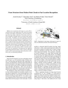
Chapter 1 Introduction There are two common ways to create digital 3D geometry: either the geometry is designed from scratch using interactive modeling software or the geometry is digitized from a physical object, for example using a 3D scanning device. The latter approach is becoming more and more popular because scanning devices deliver a high quality point-set and models are becoming more and more complex, thus more difficult and time-consuming to construct from scratch using modeling software. Figure 1.1 illustrates the process of 3D content creating using points based on model acquisition. First, some digital object is digitized using a 3D scanning device. The resulting point set is then reconstructed into a surface representation for processing and modeling. Finally, the model is displayed using some rendering method. This thesis will focus on the surface reconstruction and the rendering step. We will start this thesis by giving a detailed description of the problem: surface reconstruction, along with some subgoals we would like to accomplish and some related subproblems which need to be solved. Then some application of surface reconstruction will be discussed. This chapter will be concluded with the thesis outline for the next chapters.
1.1
Problem Statement
Given a set of n unorganized points P = {pi |pi ∈ R3 , i = 1, .., n}, reconstruct an implicit surface that approximates the given set of points P . Usually the points pi come from a sampling process, for example by using a 3D-scanner and can subject to noise. We make the following assumptions about the point set: • The samples describe the objects boundary and not its volume. This means a thin 2
Figure 1.1: The 3D point based content creation pipeline. Image courtesy of Pauly [Pau03].
point set which describes the boundary of the object. • The object is well-sampled. This means that the object is sampled with a good sampling density and that the sampling error is low, so that the original object can be reconstructed from the given point set. In this thesis implicit functions are used to reconstruct a given point set, this mean the output is a function f : R3 → R (1.1) which is the mathematical representation of the given point set, which should approximate the original object. The surface is then defined as the zero-level set of the function f � S = x ∈ R3 |f (x) = 0 .
1.1.1
(1.2)
Subgoals
Normal information. Normals are an important tool for a wide range of effects, i.e. shading and collision detection. Therefore we want to be able to compute the normal on any point on the reconstructed object. Stability and noise resistance. We want our algorithm to be stable and resistant to noise. Practically, this means that small sampling errors will not result in another surface. 3
Reconstruction of local features. We want the algorithm to be able to reconstruct local features in the original model. Fast reconstruction. We want our algorithm to reconstruct the given point set fast, which practically means that we do not want to wait a few hours/days to get a good result. Fast raytracing. With the recent advances in raytracing, near-real time rendering is possible for triangle meshes. Traditionally, an implicit function was triangulized for interactive visualization. We will try to get a fast raytraced result of the reconstructed model, using implicit functions as rendering primitives.
1.1.2
Related Subproblems
In order to accomplish our goal, a number of subproblems have to be solved: Spatial subdivisioning. Spatial subdivisioning is used to divide the space into smaller parts. These smaller parts can be used to compute local approximations, which results in better local feature reconstruction and also a faster computation. Also, spatial subdivisioning can be used to reconstruct a multi-resolution hierarchy of a model, where each new subdivision is a refinement of the old subdivision. In our implementation, a kD-tree is used as spatial subdivisioning technique. Linear system of equations. In order to compute an implicit function which approximates the point set, a linear system of equations has to be solved. The problem with these methods is that they are numerically very unstable. To obtain non-trivial solutions, Singular Value Decomposition is used. Local surface analysis. When a fitting function is chosen from a set of functions, the surface has to be analyzed in order to choose a function which most efficient approximates the local surface topology. The most important factors for surface analysis are spatial and normal distribution of the points. Distance estimation. Distance is a crucial objective measure of the quality of the fit of a function. There are a lot of different distance measurement techniques. In our implementation, the Taubin distance is used. Blending. Blending is used to construct a smooth surface by blending local surfaces together. The smoothness of the resulting global surface depends on the blending function used. 4
1.2
Applications
There is an numerous applications for surface reconstruction techniques from point sets. We will describe a few here. 3D Scanning. Scanning devices provide a high quality and high resolution point set of a scanned object. This is an alternative to modeling a virtual object using traditional modeling packages. The best known repository of 3D models is the Stanford 3D scanning repository [Rep], home of the famous Stanford Bunny. Digital Michelangelo Project. Also a project of Stanford University, the goal of this project was to create a long-term digital archive of some important cultural artifacts. Their most famous model is the David model of Michelangelo, which was digitized at a 1mm resolution, resulting in 56 million triangles. Other famous models include the St. Matthew model, represented with 372 million triangles and Atlas, represented with approximately 500 million triangles. More information can be found on their website [Pro]. Thinning Point Sets. By looking at the topology of the function which approximates a point cloud, a new point cloud can be generated which contains a more optimal point distribution which more efficiently captures the shape of the original object [ABCO+ 03]. For example, functions with a simple topology can be represented with a few points.
1.3
Thesis Outline
This thesis is organized as follows: • Chapter 2 discusses parametric and implicit surfaces, some frequently used distance metrics. Also, a mathematical foundation of least squares minimalization is given. • Chapter 3 gives an overview of different methods to construct implicit surfaces from point clouds. This chapter focuses on the techniques found in the literature, with their advantages and shortcomings. • Chapter 4 focuses on the implementation. It describes in detail the major challenges faced during the implementation together with the chosen solutions.
5
• Chapter 5 contains the results of the implementation. It visualizes the different issues discussed in chapter 4 using screenshots obtained from the implementation. • Chapter 6 concludes this thesis by summarizing the achieved results and gives an outline for future work.
6
Chapter 2 Surfaces In computer graphics a large variety of geometric representations have been used for reconstruction, modeling, editing and rendering of 3D objects. On the most abstract level these representations fall in two categories: implicit and parametric representations. These two types of surfaces will be discussed in next two sections, along with their advantages and disadvantages. Then we will discuss some frequently used distance functions, as they are very important in the reconstruction process. We conclude this chapter with a mathematical description of function fitting.
2.1
Manifolds
Mathematical foundations about implicit surfaces can be found in a lot of books [BW97, Sze04] and websites [Mat]. The most important definitions that will be given here will be analog to those given in [Sze04], some intuitive examples are inspired by [Wik]. We will review the most important mathematical concepts here, more details can be found the in referenced books. Intuitively, a manifold is a topological space that is locally Euclidean. Locally, these spaces look like spaces as described by Euclidean geometry but they can have a more complicated structure when viewed as a whole. An example of this is the surface of the earth. For a person standing on the surface seems flat, but when viewed from space, it look spherical. A manifold can be constructed by ‘gluing’ separate Euclidean spaces together. For example, a world map can be constructed by gluing many maps of local regions together. We will review some important definitions and properties to construct a mathematical 7
definition of a manifold. Definition 1 Given a set X, a topology on X consists of a family of subsets T , called open sets, which satisfy the following conditions: • The empty set φ is open and the entire space X is open, {φ, X} ⊂ T . • U ∈ T and V ∈ T ⇒ U ∩ V ∈ T • If {Vi |i ∈ I} is any family of open sets, then their union
S
i∈I
Vi is open.
Definition 2 A pair (X, T ), where T is a topology on X, is called a topological space. The elements of the underlying space X are usually referred to as points. A Hausdorff space, separated space or T2 space is a topological space in which points can be separated by neighborhoods. Or, more formally: Definition 3 Given x, y ∈ X, where X is a topological space. We say that x and y can be separated by neighborhoods if there exists a neighborhood U of x and a neighborhood V of y such that (U ∩ V ) = φ. Definition 4 A topological space X is called a Hausdorff space if any two distinct points of X can be separated by neighborhoods. For example, the real numbers R are a Hausdorff space. Also, all metric spaces are Hausdorff spaces. A homeomorphism is a special isomorphism between topological spaces which respects topological properties. Two homeomorphic spaces are identical, from a topological viewpoint. One can see a homeomorphism between two spaces as a continuous stretching and blending of one space into the other. For example, a square and a circle are homeomorphic. Intuitively, a homeomorphism maps points in the first space which are ‘close together’ to points into the second space that are close together, and vice versa. We will now define a homeomorphism formally: Definition 5 A function f between two topological spaces X and Y is called a homeomorphism if it has the following properties: • f is a bijection • f is continuous 8
• f −1 is continuous If such a function exists we say that X and Y are homeomorphic. For example, the open interval (−1, 1) is homeomorphic to the real numbers R. Definition 6 A point x = (x1 , x2 , . . . , xn ) is inside an Euclidean n-ball iff � B n = (x1 , x2 , . . . , xn ) |x21 + x22 + . . . + x2n < 1 .
(2.1)
Finally, using the definitions above, we can define a manifold: Definition 7 An n-manifold is a second countable Hausdorff topological space in which every point has a neighborhood homeomorphic to an open Euclidean n-ball. The term ‘second countable’ means that it satisfies the second axiom of countability, which states that the topology has a countable base. There are a lot of different types of manifolds. In computer graphics, differentiable manifolds are used. This is a manifold with a globally defined differentiable structure, which permits to do calculus on it. Practically this means one can define directions, tangent spaces and differentiable functions on this manifold. Each point of a n-dimensional differentiable manifold has a tangent space, this is a n-dimensional Euclidean space consisting of the tangent vectors of the curves through the point. A surface is an example of a two-dimensional manifold. The two-dimensional character of a surface comes from the fact that, around each point, there is a coordinate patch on which a two-dimensional coordinate system is defined. In general, it is not possible to extend this patch to the entire surface, so it will be necessary to define multiple patches which collectively cover the surface.
2.2
Parametric Surfaces
A parametric surface is a surface whose boundaries are defined by parametric functions: x fx (u, v) y = fy (u, v) z fz (u, v)
(2.2)
Parametric surfaces like subdivision surfaces [Zor00] or triangle meshes are based on a mapping from a (piecewise) planar domain Ω to R3 , i.e., f : Ω → R3 . The number of 9
mappings needed to accurately represent a surface tightly correlates with the complexity of its surface. Since points on the surface can be obtained by evaluating the inverse function f −1 : R3 → Ω, parametric surfaces can be rendered quite efficiently. Extreme deformations and topology changes usually require changes to the domain Ω in order to avoid strong distortions and inconsistencies. For example, the shape of a triangle mesh can be modified to a certain extend by only changing the vertex positions, but keeping the connectivity fixed. However, if the local distortions become too strong or if the surface topology changes, the mesh connectivity has to be updated, while maintaining strict consistency conditions to preserve a manifold surface structure. Intuitively, a manifold surface structure means that for every point on the surface, a valid normal can be computed. The advantage of parametric surfaces is that they are very flexible and that the parameterizations are not required to be functions. The number of parameters usually gives the object’s dimension, which does not have to be the dimension of the space. The best known examples of parametric surfaces are probably Bezier curves, which are usually triangulated for visualization. Because of their need to be triangulated, parametric surfaces are quite good for rendering purposes, but inefficient for modeling purposes, because global consistency of the mapping has to be guaranteed, or re-established if the changes are too strong. In practice, the necessity to re-establish the global consistency of the mapping makes this kind of operations on parametric surfaces rather inefficient.
2.3
Implicit Surfaces
An implicit surface is defined as the isosurface of a function f : R3 → R. In other words, it is the set of points that satisfy the equation f (x, y, z) = d
(2.3)
where d can be thought of as the density of a 3D scalar field at point (x, y, z). Usually the equation is of the form f (x, y, z) = 0 (2.4) where the following properties are defined for inside/outside detection: • d > 0 for points inside the surface, • d = 0 for points on the surface,
10
• d < 0 for points inside the surface. The biggest advantage of implicit surfaces over parametric ones is the classification of a point relative to the surface is trivial. One has only to look at the sign of the function at the given point. Also, normal computations of implicit functions are easier than for parametric surfaces. For a implicit function, the normal is defined as the unit length gradient at a point, whereas for parametric surfaces, the normal is usually computed as the cross-product of the surface tangents in the two parametric directions.
2.4
Distance Metrics
In order to define a metric space, a distance function has to be defined. First, a number of properties which all distance functions must obey is given, called the general distance function. A general distance function between two points is defined as follows: Definition 8 For all x, y, z ∈ space S, a general distance function d between these two points must satisfy: • d(x, y) = 0 ⇔ x = y, • d(x, y) ≥ 0, • d(x, y) = d(y, x), and • d(x, y) ≤ d(x, y) + d(y, z). In our context, surface fitting, the notion of how far a point is away from the surface is crucial. There are a number of popular distance metrics used to calculate the distance between a point from a surface.
2.4.1
Norms and Euclidean Distance
Given two points x = (x1 , x2 , . . . , xn ) and y = (y1 , y2 , . . . , yn ), the Minkowski distance of order p, also called the p-norm distance, is defined as: N X i=1
|xi − yi |p
! p1
v ! u N u X p |xi − yi |p . =t i=1
11
(2.5)
Figure 2.1: Various distance metrics used. Left: Euclidean distance. Right: algebraic distance. The 2-norm distance is called the Euclidean distance. When working in R3 , the Euclidean distance between two given points p = (px , py , pz ) and q = (qx , qy , qz ) is defined as: q
(px − qx )2 + (py − qy )2 + (pz − qz )2 .
(2.6)
The distance of a point p to a given surface S is then defined as the distance between the point p and the closest point on the surface from p: q (2.7) min (px − qx )2 + (py − qy )2 + (pz − qz )2 . q∈S
Finding this closest point on the surface can be an expensive operation because it tests all points on the surface. An example of the Euclidean distance between a point an a ellipsoid is given in figure 2.1 left. A drawback of using the Euclidean distance is that it works in absolute positions, i.e., the difference between two points in absolute space, and in no way incorporates information of the surface.
2.4.2
Algebraic Distance
The algebraic distance is commonly used because of its simple form. For a given implicit surface S, defined by f (x) = 0, the algebraic distance of a point p is simply defined as f (p): d(p, S) = f (p). 12
(2.8)
As a result, the distance of points near the surface will be smaller than those farther away from the surface. An example of the algebraic distance between a point an a ellipsoid is given in figure 2.1 right. Basically, the algebraic distance is the same as Euclidean distance for hyperplanes, but can have significant error for curved surfaces. To cope with this problem, a variant of the algebraic distance was produced by Taubin.
2.4.3
Taubin Distance
The Taubin distance [Tau91] is the algebraic distance divided by it’s gradient: d(p, S) =
f (p) . |∇ (p)|
(2.9)
The result of this division by its gradient is that uneven speed of distance growth is suppressed. Essentially, it is a first-order approximation of the Euclidean distance.
2.5
Least Squares Approximation
The term least squares describes a popular technique for solving overdetermined or inexactly specified systems of equations. Instead of solving the equations exactly, a minimalization of the sum of the squares of the residuals is computed. A general description of least squares approximation can be found in [PVTF02]. Here, we will focus on least squares approximations for surface fitting in R3 . Given a point set P of N points and a reference point, we want to obtain a function f : R3 → R that approximates the points pi of P which is done by minimizing the sum of the squares of the residuals. The total error E of all data points pi , approximated by a function f is given by the following equation: E=
N X
kf (pi ) − fi k2
(2.10)
i=1
This leads to the following minimalization problem: min
f ∈Πdm
N X
kf (pi ) − fi k2 ,
(2.11)
i=1
where f is taken from the Πdm , the space of polynomials of total degree m in d dimensions. For example, we can use quadratics in three dimensions, hence d = 3 and m = 2. Then, 13
f (x) can be written as f (x) = b(x)T c,
(2.12)
where b(x) = [b1 (x), b2 (x), . . . , bk (x)]T is the polynomial basis vector and c = [c1 , c2 , . . . , ck ]T the vector of the unknown coefficients, which we wish to minimize in equation (2.11). In general, the number of elements in b(x) and c is given by the formula k = (d+m)! m!d! [Lev98, Fri03]. Equation (2.11) can be minimized by setting all partial derivatives to zero, i.e., ∇E = h iT ∂ ∂ ∂ 0, with ∇ = ∂c1 , ∂c2 , . . . , ∂ck . By taking the partial derivatives with respect to the unknown coefficients c1 , c2 , . . . , ck , a linear system of equations is obtained from which c can be computed: N
X � � ∂E 2b1 (pi ) b(pi )T c − fi = 0 =0: ∂c1 i=1 N
X � � ∂E =0: 2b1 (pi ) b(pi )T c − fi = 0 ∂c1 i=1 .. . N
X � � ∂E =0: 2bk (pi ) b(pi )T c − fi = 0 ∂c1 i=1 This can be written in matrix form as follows N X � � 2 b(pi )b(pi )T c − b(pi )fi = 0
(2.13)
i=1
When divided by the constant and rearranging the terms, this gives N N X � � X T b(pi )b(pi ) c = [b(pi )fi ] , i=1
which can be solved as:
(2.14)
i=1
PN
c = PN
i=1
i=1
b(pi )fi
b(pi )b(pi )T
.
(2.15)
P T If the square matrix A = N i=1 b(pi )b(pi ) is nonsingular, i.e., det(A) 6= 0, substitution of (2.15) into (2.12) provides the fitting function f . For example, if we want to fit a quadratic, bivariate polynomial in two dimensions, i.e., d = 2 and m = 2 and b(x) = [1, x, y, x2 , xy, y 2 ], then the resulting linear system of equations looks as follows: 14
N X i=1
yi x2i 1 xi xi x2i xi yi x3i yi xi yi yi2 x2i yi x3i x2i yi x4i x2i xi yi x2i yi xi yi2 x3i yi yi2 xi yi2 yi3 x2i yi2
xi yi yi2 c1 2 2 x i yi x i yi c2 xi yi2 yi3 c3 3 2 2 x i yi x i y i c 4 x2i yi2 xi yi3 c5 xi yi3 yi4 c6
N X = i=1
1 xi yi x2i xi yi yi2
fi .
When using this approach, every point has an equal, constant weight factor, hence all points have equal influence on the resulting function f , even if they are very far away from the center of approximation. For some applications, we want the functions f to give a local approximation of the data points pi , which means that points close to the center of approximation should have more influence on the resulting function than points far away. This extension is called weighted least squares.
2.5.1
Weighted Least Squares
In a weighted least squares formulation, the error functional E now contains a weighting factor. The minimalization has the following form: min =
f ∈Πdm
N X
θ(ka − pi k) kf (pi ) − fi k2 ,
(2.16)
i=1
where θ : R3 → R assigns a weight to each point pi , based on it’s Euclidean distance from the center of approximation a, usually one of the points in P . This minimalization problem can be solved analog as for least squares, so we will not repeat it here. Most distance-weight functions only operate withing a certain radius from the center of approximation a, since points very far away will have very close to zero influence on the resulting function. By limiting the influence of these functions, only a part of the point set has to be evaluated, which results in a fully local, thus faster, calculation.
2.6
Conclusion
In this chapter, some basic terminology relevant to this thesis has been reviewed. The definition of a manifold is given, along with some examples. Further, the difference between implicit and parametric surfaces has been discussed and a motivation of why implicit functions are used has been given. The notion of distance is crucial in surface reconstruction, so we have discussed some popular distance metrics, with their advantages and disadvantages. 15
We finished this chapter with a mathematical desription of least squares approximation for surface fitting.
16
Chapter 3 Implicit Surface Reconstruction In this chapter, some popular surface reconstruction methods are discussed, along with their advantages and disadvantages. The focus lies on the way they work, not on mathematical theorems. More mathematical foundations about these methods can be found in [Wen05]. The different techniques discussed here are surface splatting, moving least squares, radial basis functions and multi-level partition of unity implicits. The biggest difference between these techniques is that radial basis functions construct one single global approximation, whereas the other techniques construct a global function by blending local functions together.
3.1
Surface Splatting
Surface splats have first been proposed for rendering purposes by Levoy et al [Lev82] and have recently been used in computer graphics by Zwicker et al [ZPvBG01]. The idea is, in order to construct a continuous surface, to let the input points grow until the whole surface is covered. Each of these grown points, now consisting of a volume and a normal, is called a surface splat. The most intuitive and simple technique is to let the points grow as spheres until there are no more holes in the surface. However the drawback of this technique is that it does not generate an optimal splat distribution and does not exploit any local surface information like curvature. The rendering of these splats results in serious rendering artifacts [WS05]. Since the processing and storage requirements are proportional to the number of splats, the input geometry should be modeled in such a way that the hole-free splat representation contains as few splats as possible. Extra care must be taken when constructing a hole-free 17
Figure 3.1: Covering all the data points with splats does not guarantee a hole-free approximation. While all points are covered, the resulting surface still contains a hole (blue). Image courtesy of Wu et al [WK04].
approximation, because covering all points does not guarantee that the constructed surface is hole-free, as illustrated in figure 3.1. Differential geometry tells us that locally, an ellipse is the best linear approximant to a smooth surface. Thus a locally optimal adaptation to the curvature of the underlying surface is provided by elliptical splats. These are defined by two tangential axes u and v and their respective radii at a point pi ∈ R3 . Optimal local approximation is achieved if the two axes are aligned to the principal curvature directions of the underlying surface and if the radii are inversely proportional to the corresponding minimum and maximum curvatures. Figure 3.2 visualizes the difference between an approximation using ellipses and one using disks. The computationally more involved intersection calculation for ellipses gets compensated by the far lower number of splats needed than when using a disk splat representation.
18
Figure 3.2: A torus approximated by surface splats, with an error tolerance of 0.2%. It is approximated using 510 elliptical splats (left and center), and by 734 circular splats (right). Image courtesy of Wu et al [WK04].
3.1.1
Optimized Sub-Sampling
Wu et al. [WK04] have described a sub-sampling technique for dense point clouds, which exploits the geometric properties of circular or elliptical surface splats. Their procedure consists of three steps: 1. Initial splat generation. First, an initial circular splat is generated for each input point pi . A number of seed points are chosen and every seed point grows by adding neighboring points, in the order of their projected distances to the seed point, until the size of the splat outgrows a user-defined value �. As an optional step, all resulting splats can be examined to check if an elliptical splat would be more optimal, depending on the curvature of the surface they are representing. In a post-processing step, it is made sure that the resulting splat representation contains no holes. 2. Greedy selection. From the whole set of candidate splats T , a subset of active splats T 0 gets chosen in such a way that the whole surface is covered. Finding this minimum subset T 0 is known to be NP-hard [CLRS01], therefore an approximation strategy, based on greedy selection, is used. For each splat in T , the area elements associated with each sample point are summed, for those sample points that are not already covered by the previously selected splats. Then in each step the splat which adds the maximum surface area is added to the active subset and all other splats in T are updated. 3. Global relaxation. There are situations where some splats are redundant, and local 19
Figure 3.3: The most left figure shows a redundant splat a, after the greedy selection procedure. It is removed in the middle left figure. The middle right figure shows a model with non-uniform splat distribution as produced by the greedy selection procedure. The most right one is the result after the global relaxation procedure. Image courtesy of Wu et al [WK04].
decisions about which splat to add to the active subset causes a non-uniform distribution of the splats. The removal of redundant splats and getting a uniform splat distribution is the goal of the global relaxation pass. See figure 3.3 for a visualization of these two artifacts.
3.1.2
Progressive Splat Generation
Recently, Wu et al. [Wu05] proposed an iterative splat generation method, which, in contrary to the method discussed above, uses the full splat geometry in the decimation criteria and error estimates. In a first step, all initial splats are computed. Then all splat merge operators are arranged in a priority queue, according to the error metric measuring errors caused by the respective operator, with the top element heaving the minimum error. Iterative operations are performed with applying the top operator and updating possibly affected operators in the queue, until the desired number of splats in reached. They use two different error metrics, the L2 metric, which is based on the Euclidean distance and the L2,1 error metric, which measures the deviation of normal directions. The quality of this multi-resolution method is nearly as good as that of the globally optimized single-resolution sub-sampling technique discussed above, while being almost three times faster. If the input geometry contains sharp features, all splats that represent such a feature 20
have to be clipped against one (for edges) or two (for corners) clipping planes that are specified in their local tangent frames. This technique is called splat culling and was first proposed by Pauly et al [PKKG03].
3.2
Moving Least Squares
The moving least squares (MLS) surfaces Levin [Lev98, Lev01] provide an approximating or interpolating surface for a given set of point samples. This is done by building a local fit for every point on the surface using higher order polynomials. They have first been applied to point-based methods by Alexa et al [ABCO+ 01, ABCO+ 03, AA03]. The moving least squares approach relies on the idea that a given point set implicitly defines a surface. The goal of moving least squares techniques is to reconstruct a smooth surface from the input surface, by minimizing the geometric error of the approximation. This is done by locally approximating the surface with polynomials. The main tool for MLS techniques is the projection operator, which projects any point near the surface onto the surface. In the following sections, we will define the projection procedure which will lead us to the definition of a MLS surface. Next we will discuss some properties of this projection procedure and investigate several algorithms to compute the projection, in terms of accuracy, numerical stability, convergence rate and the ability to represent sharp features.
3.2.1
Projection Procedure
Let points pi ∈ R3 , i ∈ {1, ..., N }, be sampled from a surface S, possibly with measurement noise. The goal of the projection procedure is to project a point r ∈ R3 near S onto a twodimensional surface SΨ that approximates pi . The actual computation of the projection operator Ψ : r → Ψ(r) is split into three steps, as explained in the following projection procedure (see figure 3.4). 1. Find a local reference plane H = {hn, xi − D = 0|x ∈ R3 } for r, with n ∈ R3 and knk = 1 is computed as the minimum of a local weighted sum of squared distances of the points pi to the plane. The weights attached to pi are defined by the weighting function θ : R+ → R+ , which is the function of the distance of pi to the projection of r on the plane H. θ must be a smooth, monotone decreasing function. Assume q
21
is the projection of r onto H, then H is found by locally minimizing N X
(hn, pi i − D)2 θ(kpi − qk)
(3.1)
i=1
Since the weights θ(kpi − qk) decreases as the distances kpi − qk increases, the resulting plane H approximates a tangent plane to S near the surface point q. In general, there may be several local minima of (3.1), we choose the one which is the closest to r. By setting q = r + tn, t ∈ R, (3.1) can be rewritten as N X
hn, pi − r − tni2 θ(kpi − r − tnk)
(3.2)
i=1
Define operator σ(r) = q = r + tn as the local minimum of (3.2) with the smallest t and the local tangent plane H near r accordingly. The local reference domain is then given by an orthonormal coordinate system on H so that q is in the origin of this system. 2. Use the reference domain for r to compute a local bivariate polynomial approximation to the surface in a neighborhood of r. Let qi be the projection of pi onto H and fi the height of pi over H, i.e., fi = hn, pi − qi i. Compute the coefficients of a polynomial approximation g so that the weighted least squares error N X
(g(xi , yi ) − fi )2 θ(kpi − qk)
(3.3)
i=1
is minimized. (xi , yi ) is the representation of qi in a local coordinate system in H. Note that, again, the distances used for the weight function are from q, the projection of r onto H. 3. The projection of r onto SP is defined by the polynomial value at the origin, i.e., Ψ(r) = q + g(0, 0)n = r + (t + g(0, 0)) n.
3.2.2
Properties of the Projection Procedure
The surface SΨ is formally defined as the subset of all points in R3 that project onto themselves. The advantage of this surface representation is that it avoids piecewise parameterizations. No subset of the surface is parametrized over a planar piece, but every single 22
Figure 3.4: The MLS projection procedure. First, a local reference domain H for the purple point r is generated. The projection of r onto H defines its origin. Then, a local polynomial approximation g to the heights fi of points pi over H is computed. In both cases, the weights point pi is a function of the distance to q. The projection of r onto g is the result of the MLS projection procedure. Image courtesy of Alexa et al [ABCO+ 03].
point has its own support plane. This avoids common problems of piecewise parameterizations for shapes, e.g., parametrization dependence, distortions in the parameterizations and continuity issues along the boundaries of pieces [ABCO+ 03]. The approximation of single points is mainly dictated by the radial weight function θ. The weight function suggested by Levin [Lev01] is a Gaussian d2
θ(d) = e− h2
(3.4)
where d is the Euclidean distance and h a fixed parameter reflecting the anticipated spacing between neighboring points. By changing h, the surface can be tuned to smooth out features of size smaller than h in S. More specifically, a small value for h causes the Gaussian to decay faster and the approximation will be more local. Conversely, large values for h result in a more global approximation, smoothing out sharp features of surface S. This is illustrated in figure 3.5.
3.2.3
Computing the Projection
Based on the definitions given above, Alexa et al [ABCO+ 03] describe a method to compute the projection. They compute the support plane H by starting with an initial normal estimation in the to be projected point r. The normal at a point might be given as a part 23
Figure 3.5: The effect of different values for parameter h of the gaussian weight function. A point set representing an Aphrodite statue defines an MLS surface. The left picture shows an MLS surface resulting from a small value and reveals a surface micro-structure. The right one shows a larger value for h, smoothing out small features or noise. Image courtesy of Alexa et al [ABCO+ 03].
of the input, or could be computed when refining a point set surface (e.g. from neighboring points in the already processed point set). If no normal is available, it is computed using the Eigenvector of the matrix of the weighted co-variances B ∈ R3×3 : bjk =
N X
θi (pij − rj ) (pik − rk )
(3.5)
i=1
After the initial normal estimation, the actual projection procedure consists of two steps, which are repeated as long as any of the parameters changes more than a user-defined value �: 1. Minimize along t, where the minimum for t is initially bracketed by t ± h2 . 2. Minimize q on the current plane H : (t, n) using conjugate gradients. The new value for q = r + tn leads to new values for the pair (t, n). The last pair (t, n) defines the resulting support plane H. The second step of the projection procedure is a standard linear least squares problem: once the plane H is computed, the weights θi = θ(kpi − qk) are known. The gradient of (3.3) over the unknown coefficients of the polynomial leads to a system of linear equations 24
of size equal to the number of coefficients, e.g. 10 for a third degree polynomial, where a non-trivial solution can be obtained using, for example, singular value decomposition [PVTF02]. � � The initial constraint for t ∈ − h2 , h2 is motivated by the assumption that a point to be projected is at most distance h2 away from its projection. Then, t will only have one local minimum in this interval. Consider the general case, a normal is computed and the function is minimized with respect to t. This is a nonlinear minimization problem in one dimension. In general, it is not solvable with deterministic numerical methods because the number of minima is only bounded by the number N of points pi . By bracketing t to this interval, this problem is avoided because there will be only one minimum. Intuitively this can be seen as h is connected to the feature size and features smaller than h are smoothed out. Therefore, the assumption is made that any point r to be projected is at most distance h away from its projection. While this might seem to be quite restrictive, in almost all 2 practical applications this assumption is naturally satisfied [ABCO+ 03].
3.2.4
Approximation Error
A MLS surface has the projection property, i.e., Ψ(Ψ(r)) = Ψ(r).
(3.6)
However, when using Gaussian kernels, the MLS projection is not interpolation but approximating. In general, this means that Ψ(pi ) 6= pi . Let P denote the set {pi }, thus the surface SΨ defined by the point set {Ψ(pi )} is different than the surface defined by the point set {pi }. In order to quantify this difference, Alexa et al. considered the approximation error of the MLS projection [ABCO+ 03]. Using the knowledge, from differential geometry, that a smooth surface can locally be represented as a function over a local coordinate system. It is also known that approximating a bivariate function f by a polynomial g of degree m, the approximation error is kg − f k ≤ M hm+1 [Lev98], where the constant M involves the (m + 1)th derivatives of f . Assuming that both surfaces have been approximated with the same scale factor h, they found that kSΨP − SP k < Mm+1 hm+1 .
(3.7)
This means, for example, that when approximating a surface with cubic polynomials that the approximation error depends on the fourth order derivatives of the surface. As a side note, the human visual system cannot sense smoothness beyond second order [Mar83]. 25
Figure 3.6: A surface that cannot be reconstructed using a fixed kernel width. (a) surface, (b) sampling pattern, (c) vertical cross-section of the surface, (d) sample spacing. Image courtesy of Pauly [Pau03].
3.2.5
Adaptive Moving Least Squares
In the above discussion, the MLS surface approximation always used a fixed Gaussian kernel with width h. However, finding a suitable h can be difficult for non-uniformly sampled point clouds. A large scale factor causes too much smoothing in regions of high sampling density and with a low scale factor, only few points will contribute significantly to the computations because the decay of the weight function. This can lead to instabilities in the optimization, which results in wrong surface approximations. Figure 3.6 shows an example of a surface that cannot be approximated adequately using a global scale factor h. The surface is defined using a concentric sine wave whose wavelength and amplitude gradually increases towards the rim of the surface, as can be seen in figure 3.6(c). Similarly, the sampling density decreases towards the boundary as illustrated in figures 3.6(b) and (d). This gives us a coupling between the surface detail and the sampling density, i.e., in regions of high sampling density the surface exhibits a lot of detail, et vice versa. Figure 3.7 shows reconstructions of the central section of this surface using the regular sampling grid shown in figure 3.7(b). The Gaussian used in figure 3.7(c) causes substantial 26
Figure 3.7: Regular re-sampling of a non-uniformly sampled surface with fixed Gaussian kernels. Image courtesy of Pauly [Pau03].
27
Figure 3.8: Adaptive MLS surface reconstruction of figure 3.7. The surface is reconstructed using the sampling pattern of figure 3.7(b). Image courtesy of [Pau03].
smoothing and leads to a significant loss of geometric detail in the central area. In figures 3.7(d) and (e), the kernel width has been halved which improves to approximations in the central region but leads to increasing instability towards the boundary. To cope with this problem, Pauly [Pau03] has proposed an adaptive MLS scheme, where the MLS approximation adapts to the local sampling density. In regions with high sampling density a small Gaussian kernel should be applied to accurately reconstruct potential high geometric detail. If the sampling density is low, the kernel width needs to be bigger to improve the stability of the approximation. In his work, Pauly proposes to extend the MLS approximation by using, instead of a fixed scale factor h for all approximation, a dynamically varying scale factor, defined as hr =
h , ρ(r)
(3.8)
where r is the point that is to be projected onto the MLS surface and ρ(r) : R3 → R a continuous, smooth function approximating the local sampling density. Computing ρ involves an estimation of the local sampling density ρi for each point pi ∈ P . This can be done building a sphere with radius ri around the point pi that contains the k-nearest neighbors to Pi . A value of k/ri2 for pi is suggested by [PKKG03]. Optionally, in a second step, ρ can be interpolated using standard scattered data approximation techniques.
3.2.6
Sharp Features
When constructing a MLS surface on a input data set by using a Gaussian kernel, we approximate the input points. A result is that sharp edges are smoothed out. For example, 28
take figure 3.9, where the input points can either be interpreted as defining a smooth surface or as defining a sharp surface. The techniques discussed above always produce a smooth surface. But sometimes we want sharp features to be accurately represented, not smoothed out. Points on sharp features are defined by multiple surfaces, thus dealing
Figure 3.9: Noisy input data can either represent a sharp surface (a) or a smooth surface (b). Image courtesy of Fleishman et al [FCOAS03].
with sharp features requires fitting a number of surfaces locally [PKKG03]. If the point data set contains reliable normals, they can be used to differentiate between local surfaces [OBA+ 03]. However, using normals to identify a discontinuity is mostly not applicable, since the definition of a normal requires local smoothness and its computation in the presence of noise or near a discontinuity in unreliable. The term discontinuity refers to the discontinuities in the derivative of a surface. Fleishman et al [FCOAS03] describe a technique to represent sharp features without normal information. Their work is based on a statistic technique called the forward search paradigm [AAC00]. The idea is to start from a small set of robust samples of the input data that excludes outliers. From this initial subset we move forward through the data, adding points to the subset while monitoring certain statistical estimates. These estimates are used to deal with noise, outliers and sharp features. Instead of fitting a single surface locally by the MLS algorithm, an iterative refitting algorithm is used, based on the forward search algorithm, to classify a neighborhood to multiple local surfaces. Points which are close to more than one local surface are projected on one of its neighboring smooth regions. The local classification along with a new projection procedure defines a piecewise smooth surface, where each region is infinitely smooth. The least medians of squares (LMS) is a regression method that estimates the parameters β of the model, by minimizing the median of the absolute residuals. These residuals 29
are defined as the difference between the measurement and estimation: ri = f (xi ) − yi . We search the parameters β that minimizes the median of the residuals. This problem can be solved using the following random sampling algorithm: 1. Select k points at random, and fit a model to the selected points. 2. Compute the median ri , β of the residuals of the remaining N − k points. 3. Repeat the previous 2 steps T times to generate T candidate models. 4. Select the model with minimal ri , β as the final model. The iterative fitting procedure goes as follows: 1. Fit a model to a subset S1 of the data, using the forward search algorithm and identify the rest of the data as outliers. 2. Remove the samples that were fitted from S. 3. Repeat the previous steps until S is empty. This procedure is visualized in figure 3.10 for the two dimensional case. To deal with sharp features, a new projection operator is introduced. It projects a point onto a piecewise smooth surface using the classification process described above. This classification process allows to project points on a locally smooth region rather than a surface that is smooth everywhere, thus defining a piecewise smooth surface. By treating the points across discontinuities as outliers, sharp features can be represented. Given a point x, first it is analyzed if its neighborhood is smooth. If it is, Levin’s projection method is used. Otherwise this neighborhood of points is classified to subsets of smooth regions of the surface and outliers are discarded. If the neighborhood is not smooth, a subset of the neighborhood that is sampled from a smooth region of the surface is used. A forward search procedure is applied to obtain a subset of the neighborhood that samples a smooth region. The rest of the smooth regions are then obtained by the iterative refitting procedure. The result is a classification of the neighborhood into one or more subsets, as can be seen in figure 3.10(e). In the case that there is only one subset, the rest of the points are outliers and are simply discarded and projected as if it were a smooth region. When there are two or more subsets, the surface is defined as the intersection of the smooth surfaces defined by the different neighborhoods. The new projection works by first projecting x on one surface and then use another surface to check if the points belongs 30
to the intersection or not. In the case the point belongs to the intersection, the surface is chosen that is closest to x, as shown in 3.11(a). In case none of the points belong to the intersection, as in figure 3.11(b), they iterate on this process until we converge to the edge, as Pauly et al [PKKG03]. To check if a point that was projected on one surface agrees with the other surface, first is determined if the neighborhoods form a convex or concave region and then use this information to make inside/outside tests. Find the closest point to the two rays that are defined by these representative points and their normals, see figure 3.11(c). If that point is inside the object then the region is convex, otherwise it is concave. The same principle applies when dealing with more than 2 surfaces.
3.3
Radial Basis Functions
Radial basis functions (RBF) are known for a long time as one of the most accurate and stable methods to solve the scattered data interpolation problem. Only very recently have radial basis functions been used within the computer graphics domain [TO99, CBC+ 01, MYC+ 01]. Radial basis functions are functions where the outcome is rotation invariant around a certain point. They can be used to interpolate a function with n points by using n radial basis functions, centered at these points. Thus, the resulting interpolated functions becomes n X λi φ(kx − pi k) (3.9) f (x) = i=1
where pi is the position of the known values, i.e., the input points and λi is the weight given by the radial basis function centered at that point. Essentially, as Carr et al [CBC+ 01] pointed out, there are 2 major steps in a procedure to reconstruct a sparse sampled surface with radial basis functions: 1. Construction of a signed distance function. 2. Fitting of a radial basis function to the resulting distance function. Figure 3.12 shows the plot of some widely used radial basis functions. In the following sections, each of these steps will be discussed in detail.
31
Figure 3.10: An overview of the identification of sharp features using the iterative refitting procedure. Image courtesy of Fleishman et al [FCOAS03].
Figure 3.11: Projection of points onto the surface near an edge, using convex/concave information. Image courtesy of Fleishman et al [FCOAS03].
32
Figure 3.12: Plots of various widely used radial basis functions. Image courtesy of Morse et al [MYC+ 01].
3.3.1
Signed Distance Function
The goal of the reconstruction process is to find a function f which implicitly defines a surface S and satisfies the equation f (pi ) = 0,
(3.10)
for each pi ∈ R3 lying on the surface S. The trivial solution to this interpolation problem is a function that is zero everywhere. To avoid this trivial solution, off-surface points are added to the input data set and are given non-zero values. This gives us the following interpolation problem: find a function f that satisfies the following conditions: f (pi ) = 0 ∧ f (oj ) = dj
(3.11)
with oj an off-surface point and dj 6= 0. Carr et al [CBC+ 01] describe a method to generate off-surface points oj and their corresponding values dj . For f they choose a signed distance function, with dj the Euclidean distance to the closest point on the surface. The off-surface points are generated by projecting along the surface normals, similar to Turk et al [TO99]. Experiments have shown that is it best to generate off-surface points on both sides of 33
Figure 3.13: Reconstruction of a hand point cloud. Figure (a) shows the original point cloud (green), augmented with off-surface points on the outside of the surface (red) and on the inside (blue). When using a static projection procedure to generate the off-surface points, errors in the vicinity of the fingers become visible because opposing normal vectors have intersected (c). Using dynamic projection to generate the off-surface points eliminates these problems (b). Image courtesy of Carr et al [CBC+ 01].
the surface. Points outside the surface are assigned a positive value and points inside the surface are assigned a negative value. This leaves us with two sub-problems. First an estimation of the surface normals and secondly a calculation of the projection distance. In general, it is very difficult to make a robust estimation of the normals over the whole surface. When no robust estimation for a normal is available, no normal is fitted at that point. The data point, which is a zero-point, will tie down the function in that region. When all normal information is available, off-surface points must be projected along the normal direction. Care must be taken that they do not intersect other parts of the surface. Projected points must be constructed so that the closest on-surface point is the surface point that generated it. Therefore projecting off-surface points a fixed distance from the surface can lead to errors, as can be seen in figure 3.13(c). By using a dynamic projection, these errors are avoided, as illustrated in figure 3.13(b).
3.3.2
Fitting of the Signed Distance Functions using RBF
The general formulation of a radial basis interpolated function was given in (3.9). However, in some cases, it is necessary to add a first-degree polynomial P to account for the linear and constant portions of f and ensure positive-definiteness of the solution. This gives us
34
the following formulation: f (x) =
n X
λi φ(kx − pi k) + P (x).
(3.12)
i=1
To solve this equation for the set of weights λi that satisfy the constraints f (pi ) = di , each pi is inserted in equation 3.12: f (pi ) =
n X
λi φ(kpi − pj k) = di
(3.13)
λi φ(kpi − pj k) + P (pi ) = di
(3.14)
j=1
or if a polynomial is required: f (pi ) =
n X j=1
Equation 3.13 can be written in matrix notation as follows: λ1 φ11 φ12 . . . φ1n φ21 φ22 . . . φ2n λ2 . .. . . . . = . . .. . .. . φn1 φn2 . . . φnn
and equation 3.14 as φ11 φ12 φ21 φ22 .. .. . . φn1 φn2 x p1 px2 y p1 py2 pz pz 1 2 1 1
. . . φ1n px1 py1 pz1 . . . φ2n px2 py2 pz2 .. .. .. . . . .. . . . . x y . . . φnn pn pn pzn . . . pxn 0 0 0 . . . pyn 0 0 0 . . . pzn 0 0 0 1 1 0 0 0
λn
1 1 .. . 1 0 0 0 0
λ1 λ2 .. . λn px py pz 1
d1 d2 .. . dn
(3.15)
=
d1 d2 .. . dn 0 0 0 0
(3.16)
where φij = φ(kpi − pj k). The matrix in these equations is obviously symmetric and with proper selection of basis functions it can be made positive-definite [MYC+ 01]. Thus, a solution will always exist for this problem.
3.3.3
Global vs Compact Support
Morse et al [MYC+ 01] analyzed some computational properties of radial basis functions with global support, for example a thin-spline like in figure 3.12(b): 35
• O(n2 ) computation is required to build the system of equations. • O(n2 ) storage is required (for the nearly full matrix) to represent the system. • O(n2 ) computation is required to solve the system of equations. • O(n) computation is required per evaluation • As every point affects the result, a small change in one point affects the entire resulting surface. A logical extension is to make radial basis functions with compact support radius. Whenever a certain point is more than a distance r away from a reference point, its contribution is set to zero. Wedland [Wed95] has developed a minimum-degree polynomial solution for locally supported radial basis functions that guarantee positive-definiteness of the matrix. These are called compactly supported radial basis functions. THese functions have the following form: ( (1 − r)p P (r) if r < 1 φ(r) = (3.17) 0 otherwise All these functions have support radius equal to one. These can be scaled to support any desired radius α by scaling the basis functions, i.e., φ( αr ). During computation, this means that all points that lie within a given distance from a reference point have to be found. This can be done, by using a kd-tree, in O(log n) time. When using compactly supported radial basis functions, the matrix contains a lot of zero-entries. Thus we can use a sparse matrix solver to find the solution to the system of equations, which can now be solved in time complexity O(n1.5 ) [MYC+ 01]. Figure 3.14 visualizes the difference between the number of zero-entries in the matrix between radial basis functions with local and global support. As a summary, we will compare some properties between globally and locally supported radial basis functions: Global support Local support Computation to build O(n2 ) O(n log n) Computation to solve O(n2 ) O(n1.5 ) Storage to build/solve O(n2 ) O(n) Computation to evaluate O(n) O(log n) Effect of a single point global local
36
Figure 3.14: The structure of the matrices produced by global and local supported radial basis functions. The globally supported, thin-spline, basis function (left) produces a matrix that is nearly full (white), while compactly supported radial basis functions produce a matrix that is sparse (black). Image courtesy of Morse et al [MYC+ 01].
3.3.4
Multi-scale Approach
Ohtake et al [OBS03] have proposed a hierarchical approach to 3D scatted data interpolation using compactly supported basis functions. Their ideas were motivated by Kojekine et al [KHS03] who showed that, when using an appropriate carrier implicit surface, fitting scattered data with compactly supported radial basis functions can be done very fast. They let the coarser levels in the hierarchical approach serve as the carriers for finer levels. The hierarchical approach makes their method insensitive to the density of scattered data and allows for reconstruction of large parts of missing data. A new type of compactly supported basis function is introduced: quadrics multiplied by compactly supported radial weights, where the quadric coefficients are determined via local weighted least squares fitting and via a global interpolation procedure. First will be discussed how the interpolation works at a single level. 3.3.4.1
Single-Level Interpolation
Given a set of P = {pi } consisting of N points and equipped with unit normals ni defining an orientation, a 3D scalar field f (x) is generated such that its zero-level set f (x) = 0 separates the space into two pars. Assume f (x) has negative values outside the surface
37
and positive inside. The interpolation of the point set P is given by: f (x) =
N X
[gi (x) + λi ] φσ (kx − pi k) ,
(3.18)
i=1
� where φσ (r) = φ σr and φ (r) = (1 − 4)4+ (4r + 1) is Wendland’s compactly supported RBF [Wed95], σ its support size. The gik (x) and λi are the unknown function and coefficient to be determined. These are chosen by the following procedure. 1. At each point pi , the function gi (x) is defined such that it’s zero-level set locally approximates the shape of P . 2. The coefficients λi are determined from the interpolating conditions f (pj ) = 0 =
N X
[gi (pj ) + λi ] φσ (kpj − pi k)
(3.19)
i=1
and thus leads to a sparse system of linear equations with respect to λi . The interpolation matrix is positive definite because Wendland’s compactly supported RBFs are strictly positive. The parameter σ is estimated form the density of P . Details of the interpolation procedure can be found in [OBS03]. 3.3.4.2
Multi-Level Interpolation
� In order to construct a multi-scale hierarchy of point sets P 1 , P 2 , . . . , P M from P , P is fit into a parallelepiped and its parts are recursively subdivided into eight equal octants. For all points contained in a cell, their centroid is computed, along with a unit normal for the centroid, obtained by averaging the normals assigned to the points inside the cell. The set P 1 corresponds to the subdivision of the parallelepiped into eight equal octants, P 2 the subdivisioning of each cell of P 1 , . . . . This approach is visualized in figure 3.15. After constructing the hierarchy, the multi-level interpolation procedure proceeds in a coarse-to-fine way. First, a basis function f 0 (x) = −1
(3.20)
is defined, and then recursively the set of interpolation functions f k (x) = f k−1 (x) + ok (x) 38
(3.21)
Figure 3.15: Multi-scale interpolation overview. A monk model consisting of 60K points is obtained as laser scanner data. Top row: multi-scale hierarchy of points where the radii of the spheres at each level k are proportional to σk , the support size of the RBFs used for the interpolation. Note that the actual size of the spheres are 5 times larger than these used for visualization. Middle row: interpolating implicit surface polygonized at each level of the hierarchy. Bottom row: cross-sections of the interpolating. The bold black lines correspond the the zero-level sets of the functions. Image courtesy of Ohtake et al [OBS03]
39
are defined, for k = 1, 2, . . . , M , where f k (x) = 0 interpolates P k . An offsetting function ok has the form used for single-level interpolation. The local approximations gik (x) are defined similar the single-level interpolation, via least square fitting applied to P k , while the coefficients λki are found by solving the following system of linear equations: f k−1 (pki ) + ok (pki ) = 0.
(3.22)
The support size σ k us defined by σ k+1 = σ2 , with σ 1 = cL, where L is the length of a diagonal of the bounding parallelogram and the parameter c is chosen such that an octant of the bounding box is always covered by a ball of radius σ 1 centered somewhere in the octant. The number of subdivision levels M is determined by σ 1 and σ 0 , the support size for the single-level interpolation. A suggested value of M by [OBS03] which gives good � 0� σ results is M = − log2 2σ1 .
3.4
Multi-level Partition of Unity
Ohtake et al [OBA+ 03] present another method for implicit surface reconstruction, using a technique called multi-level partition of unity (MPU). The basic idea of a partition of unity is to break the input data domain into several pieces, where every subdomain is approximated independent from other subdomains. The local approximations are then blended together using smooth, local weights that sum up to one over the whole domain. This partition of unity method will now be expressed more formally.
3.4.1
Partition of Unity
Consider a bounded domain Ω in space and a set of non-negative compactly supported functions {ϕi } such that the sum of these functions sum to one over the whole domain. We can associate a local approximation set of functions Vi with each subdomain that is in the support range of ϕi . Then, a global approximation of a function f is given by: X ϕi (x) Qi (x) (3.23) f (x) = i
where Qi ∈ Vi . Let {wi } be a set of non-negative compactly supported functions such that Ω⊂
[
supp (wi )
i
40
(3.24)
with supp (wi ) the support range of wi , then partition of unity functions {ϕi } can be generated: wi (x) ϕi (x) = PN . (3.25) j=1 wj (x) This approach gives more freedom in the choice of local shape functions, so it is possible to accurately represent sharp features by selecting appropriate shape functions. Basically, there are three ingredients: 1. Piecewise functions that capture the local shape of the surface. 2. Non-negative compactly supported weighting functions that blend the local shapes together. 3. An error-controlled subdivision method that adapts to variations in the complexity of the local shape, whose time and memory requirements depends to the desired accuracy. To get a better feeling of this technique, we will briefly discuss an actual implementation of this technique, as proposed in [OBA+ 03].
3.4.2
Adaptive Octree-based Reconstruction
The core of the MPU implicit generation is subdivisioning of the input data domain, given by a set P of points. To accomplish this spatial subdivisioning, an octree with axis aligned cells is used. The root cell of the tree is the box that contains all the input data points, rescaled so that this cell has a main diagonal of length 1. The support radius for a local weight function is proportional to its diagonal, R = αd, with d the length of the main diagonal of the cell. A large value for α yields smoother interpolation and approximation results, at the expense of computation time. An α value of 0.75 is suggested by the authors. For each cell generated during the subdivisioning process, a local function Q(x) is computed using a least-squares fitting procedure (see section 3.2). If there are not enough data points inside the support radius of the support function for a robust estimation of Q(x), the support function can be expanded until there are enough points to make a robust fit. Otherwise, a local max-norm approximation error is estimated; if this error is greater than a user-defined error �0 , the cell is subdivided and the procedure is performed on all child cells, otherwise this cell is not subdivided and the cell is marked as a leaf.
41
Figure 3.16: The difference in point and normal distribution when a a bivariate quadratic polynomial (left), or a general 3D quadric (right) is used. Image courtesy of Ohtake et al [OBA+ 03].
3.4.3
Local Shape Fitting
Different types of functions are used to approximate the points in a cell, based on the distributions of the normals of those points. We will only describe briefly when they are used, for the actual computation details, the reader is referred to [OBA+ 03]. The used functions for approximation are: • a general 3D quadric, • a bivariate quadratic polynomial in local coordinates, • a piecewise quadric surface that fit an edge or corner. The general 3D quadric is used to approximate larger parts of the surface, when we have a sufficient number of data points and the difference between the average normal direction of the supported points and the maximum deviation of the normals to the average is more than Π2 degrees, if the difference is less or equal than Π2 degrees. See figure 3.16 for a visualization. If there are not enough enough points for the previous two methods, a feature detection procedure is used to check if there is a local feature given by the data points. If the feature detection procedure fails to find a local feature, a bivariate quadratic polynomial in local coordinates is still used.
42
3.5
Conclusion
In this chapter, a number of popular scattered data approximation techniques have been discussed. Surface splats are popular because they can be visualized on a GPU. However, generating an optimal splat distribution is a non-trivial task and is computationally very intensive. There is also almost no control about the continuity of the reconstructed surface, and reconstruction properties hardly exist for surface splats. Moving least squares techniques are a local technique where only neighboring information is used to construct a surface near a point. This makes it computationally fast and the locality of the neighborhood is reponsible for the reconstruction properties. Also, the continuity of the surface can be chosen, as it is the same as the kernel function used. If sharp edges need to be reconstructed, the method becomes computationally more demanding. Radial basis functions is a global technique, with the drawback that local features will be lost. However, this global property of radial basis functions makes them perfect for reconstruction properties. Disadvantages of radial basis functions are that the generation of off-surface points must be done very carefully and that it is computationally very expensive. Recently, there are multi-level methods using radial basis functions, which results in a less global but computationally more efficient representation. Multi-level partitioning of unity implicits try to approximate data by using a set of functions. This is advantageous because it can adapt itself more efficient to some local topology, while still preserving good reconstruction properties. Also, sharp edges can be reconstructed without much extra computation.
43
Chapter 4 Implementation This chapter focuses on the implementation. All used techniques and problems encountered during the implementation are discussed. This chapter is split into two sections, the first section discusses the reconstruction phase and the second one discusses the visualization. The reconstruction process is inspired by the Multi-level Partitioning of Unity method from Ohtake et al [OBA+ 03], where the model is subdivided and each subdivision is approximated using an implicit function chosen from a set of fitting functions. The partitioning of the space is realized using a kD-tree and the set of fitting functions consists of second order bivariate and general quadrics. The second section discuses the visualization of the reconstructed model, which is done using raytracing. The kD-tree constructed for the reconstruction phase is used for the raytracing process. An analytic intersection point is computed between the implicit function in a cell and a ray. This chapter discusses various implementation issues. It describes all used techniques in detail, motivates why certain choices are made, gives a descriptions of the problems encountered and the solutions used to solve them. To summarize, the following techniques are the same as seen in the literature, see chapter 3: • Set of functions. This was inspired by the Multi-level Partitioning of Unity method. Also, the tests which decide which function to used is the same as the one proposed by Ohtake et al [OBA+ 03] • Weighted least squares fitting. This is a standard technique for data approximation. Also, the used distance-weight functions are the same as those found in the literature. 44
• Improved fitting of general quadric. In their work, Ohtake et al [OBA+ 03] have described a method which improves the fitting of a general quadric. This technique is implemented. • Solving linear systems of equations. To obtain a non-trivial solution from a linear system of equations, singular value decomposition [PVTF02] is used, which is regarded as the most stable algorithm. While the following techniques all exist in literature, as far as we know these have not been applied to the domain of surface reconstruction from point clouds. Therefore, we will credit them as own contributions. • kD-tree. To our knowledge, the most frequently used subdivisioning techniques are octrees or (hierarchical) bounding spheres. Inspired by the work of Havran [Hav00], we have decided to use a kD-tree as a spatial subdivisioning method for it’s ability to efficiently adapt itself to the scene distribution. • Fast raytracing. Very frequently, a reconstructed model is triangulated for rendering purposes. In our implementation, we have decided to keep implicit functions as rendering primitives. Because the functions are of second degree, an analytic intersection calculation is possible, which eliminated the need for slower, iterative intersection algorithms.
4.1
Reconstruction
In this section, the techniques used during the reconstruction phase are discussed. First, the chosen spatial subdivisioning technique, a kD-tree, is reviewed. Then, the fitting procedure for the functions in the set of fitting functions, used to locally approximate the points, is discussed, along with the statistical analysis which decides which function is chosen for approximation. This section will be concluded with a discussion of the implemented distance-weight kernel functions.
4.1.1
Spatial subdivisioning
When a point cloud is given as input, the cloud is uniformly rescaled that it points fit into a unit cube. A kD-tree is then constructed to subdivide this cube into smaller parts, called cells, where each new subdivision splits the old subdivision by an axis aligned plane, called the splitting plane. All points inside a subdivisioning cell are then approximated using a 45
function, chosen from the set of fitting functions, based on the distributions of the points and their normals in the cell. The biggest difference between a kD-tree and an octree is the control over the position of the splitting plane. When using an octree, the splitting plane is always placed at half the length in a dimension, for all dimensions at once. For a kD-tree, the splitting dimension and splitting position can be chosen. This makes the structure of a kD-tree more dynamic than an octree, thus a kD-tree can adapt itself much better to the scene geometry. Especially when the geometry distribution is irregular, a kD-tree outperforms an octree. Because of the dynamic properties of a kD-tree, some heuristics have been developed to give the tree certain properties. For example, an octree can be created when placing the splitting plane at the half of each dimension and splitting all dimensions at once. A more sophisticated heuristic, called Surface Area Heuristic (SAH) [Hav00], has been applied to triangle meshes by Wald [Wal04] with great success. It almost doubles the performance when rendering the triangle mesh using a SAH build kD-tree than when using a tree constructed with the spatial median heuristic, which just splits a cell in half, in the dimension where it is the biggest. Essentially, int he domain of surface reconstruction and raytracing, there are two types of heuristics: • Reconstruction heuristics. By analyzing the distribution of the points and their associated normals in a cell, an efficient split position can be calculated, which gives better results, i.e., the point cloud is reconstructed using less implicit functions. • Visualization heuristics. By using a cost model, some operations become more expensive than others. For example, the average cost of computing an intersection calculation between a ray and an implicit function is more expensive than traversing one more level in the hierarchy, where a part of the cell is marked as empty, thus resulting in a faster rendering. An example of a reconstruction heuristic is shown in figure (4.1). When a function is fitted through the points in the cell (left), the error is too big thus the cell is subdivided. When using an octree subdivision (middle), the subdivisioning happens without taking any point information into account. When using a more complex heuristic, which uses more advanced statistical methods to measure the distributions of the points and their normals in a cell, a better split position can be obtained (right), which results in a more effective reconstruction procedure. An example of a visualization heuristic is shown in figure (4.2). While the reconstruction is small enough, there is still room for improving the rendering. As the intersection 46
calculation between a ray and a function is more computationally intensive than calculating the intersection the intersection between a ray and an empty cell, a heuristic can be applied that favors the creation of empty cells. While this does not result in better reconstruction quality, it achieves faster raytracing. In our implementation, only the spatial median heuristic is implemented. In time, we hope to construct a more sophisticated heuristic to better capture the local surface. The drawback of using more sophisticated heuristics is that they require more computation time.
4.1.2
Least Squares Fitting
Locally, the points inside a cell are fitted by an implicit function. This fitting process is done using the weighted least squares method, similar to the moving least squares method discussed in section 3.2. However, there are some significant differences. The MLS technique visits every point of the point set and a surface is computed which locally approximates the neighboring points, using a distance-weight function which makes neighboring points more influential than points far away. In our implementation, we are given a cell containing a numnber of points, where a function that approximates all points in the cell should be computed. This means a center of approximations has to be chosen, which is crucial because it is the center of the distance-weight function, thus defining the resulting surface topology. We want the center of approximation to be ‘near’ the points in the cell. The center of the cell is not necessarily a good center of approximation, since there is no guarantee that the center of the cell will be a good reference point. Therefore, as a center of approximation, the weighted average c˜ of all points in a cell is used: PN θ(kc − pi k)pi c˜ = Pi=1 , (4.1) N θ(kc − p k) i i=1 where c is the center of the cell and θ a distance-weight function. When needed, the weighted normal is also computed using the weighted average of all normals: PN θ(kc − pi k)ni , (4.2) n ˜ = Pi=1 N i=1 θ(kc − pi k) The rest of the fitting procedure goes as discussed in section 2.5. As observed by [XWH+ 03, OBA+ 03], all types of quadric surfaces can be divided into two groups: bivariate quadrics and general quadrics. Bivariate quadrics consist of elliptic 47
Figure 4.1: Adaptation of subdivisioning methods for reconstruction. Left: the input point set. Middle: Subdivisioning using an octree, no point distribution is taken into account. The points in the cell can be reconstructed using at least 4 functions. Right: Subdivisioning using a kD-tree, where the point distribution is taken into account. By using only one subdivisioning, the points in the cell can be reconstructed using only two functions.
Figure 4.2: Left: the input point set, fitted by a function, where a big part of the cell is empty. Right: Using one more subdivisioning level, the call can be subdivided in one emty cell, and one containing the function. This results in rendering speed-ups.
48
paraboloids, hyperbolic paraboloids, parabolic cylinders and planes. General quadrics consist of all other types of surfaces. The difference between these two groups is that bivariate quadrics are used to capture locale shapes with a simple topology that can be projected to a plane, where the topology is represented as a height function over the plane. General quadrics are used to capture more complex shapes like ellipsoids or hyperboloids. A simple test mechanism is used to decide which type of quadric will be used to approximate the point set P . Let |P | be the number of points in P , and let Nmin be a user-defined number which represents the minimum number of points in a cell. Further, let θ be the maximal angle between the normals ni of all points in the pointset P . Then, a general quadric is fit if: • |P | > Nmin and θ ≥ Π/2 otherwise, a bivariate quadric is fitted. Thus, a bivariate is fitted when: • |P | > Nmin and θ < Π/2, or • |P | < Nmin The fitting of these two classes of functions will be discussed in the next two subsections. 4.1.2.1
Bivariate Quadric
As mentioned earlier, bivariate quadrics are used when the local shape has a simple topology, which can be projected to a plane where the local shape is represented as a height function over this plane. Formally, we have defined a simple topology of the points if the maximal angle between the normals of all points in the point set is lower than Π2 . The origin of this plane is placed at the center of approximation c˜, and the height over this plane is defined by the average normal n ˜ of the points. Using this information, a right handed orthonormal base is constructed at the plane origin, where the height over this plane is defined by the weighted normal n ˜. 3 The function g (x) : R → R describes the distance of a point p to the weighted average c˜ projected along it’s normal direction n: g (x) = hn, c˜ − p0 i
49
(4.3)
where p0 = (u, v, w) is the projection of point p in the local base. Then, a bivariate quadric is given by the following equation: u a c d h i (4.4) u v 1 c b e v − w = 0. 1 d e f which can be expanded to the following equation: f (u, v, w) = (au2 + 2buv + cv 2 + 2du + 2ev + f ) − w = 0
(4.5)
where the unknowns [a, b, c, d, e, f, g]T are given by minimizing of the following equation: N X
wi f (ui , vi , wi )2
(4.6)
i=1
which results in the following linear system of equations: 1 xi yi x2i xi yi yi2 x2i yi xi yi2 x2i xi yi x3i xi N X yi xi yi yi2 x2i yi xi yi2 yi3 wi 2 3 2 4 3 2 2 x x x y x x y x y i i i i i i i i i i=1 xi yi x2i yi xi yi2 x3i yi x2i yi2 xi yi3 yi2 xi yi2 yi3 x2i yi2 xi yi3 yi4
a b c d e f
N X = w i i=1
1 xi yi x2i xi yi yi2
which, in our implementation, is solved using Singular Value Decomposition [PVTF02]. 4.1.2.2
General Quadric
Using the formulation used by Glassner [Gla89], a quadric surface is defined by the following equation: a b c d x h i b e f g y (4.7) x y z 1 = 0. c f h i z d g i j 1 when expanded, this gives the following equation: F (x, y, z) = ax2 + 2bxy + 2cxz + 2dx + ey 2 + 2f yz + 2gy + hz 2 + 2iz + j = 0
(4.8)
Fitting data points pi = (xi , yi , zi )T is done by solving the linear system of equations: ax2i + 2bxi yi + 2cxi zi + 2di xi + eyi2 + 2f yi zi + 2gyi + hzi2 + 2izi + j = 0. 50
(4.9)
where i goes through all data points pi , which can be solved using standard numerical techniques. Ohtake et al. [OBA+ 03] have described a technique which improves the fitting of a general quadric. It uses a set of auxiliary points Q = {q1 , . . . , qk } to help orient the local shape. These points are placed at the corners and at the center of a subdivisioning cell. Each of these points is tested if it can be used to obtain a reliable estimate of the signed distance function. For each point qj , it’s k nearest neighbors p1 , p2 , . . . , pk are computed from the point set P . Then, for j = 1, 2, . . . , k, the scalar products nj · (q − pj )
(4.10)
are computed. If not all scalar products have the same sign, the point qj is removed from the set of auxiliary points Q. For the remaining auxiliary points, the average distance d is computed as the arithmetic mean of the scalar products: k 1X d= nj · (q − pj ) (4.11) k j=1 The unknowns of the general quadric are then found by minimizing: N m 1 X 1 X 2 P wi (kpi − ck)f (pi ) + (f (qj ) − dj )2 wi i=1 m j=1
(4.12)
where m is the number of points remaining in the auxiliary point set Q. In our implementation, motivated by [OBA+ 03, Uhe05], a number of k = 6 is used.
4.1.3
Distance-Weight Functions
The use of distance-weight functions, sometimes called kernel functions, is crucial in the reconstruction process because it defines the smoothness of the resulting function [Lev98, ABCO+ 03]. In our implementation, three different distance-weight functions are implemented: • Linear, which results in a C 0 continuous function: 1 − kc−pi k if kc − p k < r i r θ(kc − pi k) = 0 otherwise 51
(4.13)
Figure 4.3: Plots of the three types of distance-weight functions used.
• Quadratic b-spline of degree 2, which results in a C 1 continuous function: � � �2 � kc−pi k 3 1−3 if kc − pi k < 3r r 4 � � θ(kc − pi k) = 9 1 − kc−pi k if 3r < kc − pi k < r 8 r 0 otherwise • Gaussian, which is infinite continuous: 2 ik e −kc−p h2 θ(kc − pi k) = 0
if kc − pi k < r
(4.14)
(4.15)
otherwise
where h determines the feature size. The difference between these functions is visualized in figure 4.3. Note that all used functions are compactly supported radial basis functions.
4.2
Raytracing
The visualization of reconstructed model is done using raytracing [Gla89]. One of the most used techniques to visualize a reconstructed model is to triangulate it again [OBA+ 03, Uhe05], for example using Bloomenthals polygonizer [Blo94], which can then be rendered using conventional rasterization techniques at interactive framerates. Our choice to use raytracing was based on the following motivations:
52
• Implicit functions as rendering primitives. We want to keep using implicit functions as rendering primitives. Triangulating the surface is an extra conversion, which takes additional computation time. • Scalability. Raytracing scales O(logn) with the number of primitives, whereas rasterization techniques scale O(n) with the number of primitives in the scene. When using very large models, scalability with the number of primitives becomes an important issue. • Speed. Raytracing is always seen as a non-interactive visualization technique, most of the time taking hours to compute a result. As shown recently by Wald [Wal04], raytracing can be optimized to achieve near-interactive framerates at a single computer. The implicit functions used are low order (degree two), which allows for an algebraic intersection calculation, thus eliminating the need for iterative, slower implicit function intersection methods [Har93]. First, the use of the kD-tree, constructed during the reconstruction phase, for raytracing will be discussed. Some issues will be discussed, the sampling density and the intended intersection point. Then, the intersection algorithm between a ray and a general and bivariate quadric is given.
4.2.1
Spatial Subdivisioning
The kD-tree, build during the reconstruction phase, is used during the raytracing. Every cell of the kD-tree has its own implicit function, which is an approximation of the points in that cell. Only the implicit function is stored and not the points, thus we have effectively transformed from points to implicit as primitives. When a ray intersects a cell, the intersection between the ray and the function in that cell is computed. However, there are some issues when using the kD-tree for raytracing: • Sampling density. The cells in the kD-tree fit the points as tight as possible. This requires a good sampling density of the point cloud. If the sampling is not dense enough, the reconstructed implicit function will not completely lie inside the cell, resulting in some intersection points lying outside the cell, which will not be seen as valid intersection points. • Intended intersection point. Sometimes there are two intersection points between a ray and a quadric. Care must be taken when computing the intersection point, as 53
the nearest intersection point might not be the right one. As long as one of the intersection points lies outside the cell, a valid intersection point can be calculated. But from the moment they both lie inside the cell, it is impossible to know which intersection point is the intended one, especially since no point information is available in the cell. • Numerical Stability. When a cell is very small, the resulting function will also have very small parameters, which leads to numerical instabilities during the intersection calculation procedure, resulting in visual artifacts in the visualization. These issues will be discussed next. 4.2.1.1
Sampling Density
When a function is sampled dense enough, the resulting implicit function will lie completely inside the cell. However, if the sampling density is not dense enough, it can happen that a part of the reconstructed implicit function lies outside the cell, because cell fits the points as tightly as possible. As a result, some intersection points between a ray and the implicit function will lie outside the cell, thus they will not be validated as valid intersection points. By allowing the intersection point to lie a certain distance outside the cell, this problem is partly eliminated. However, the problem with this method is that a ray just missing the cell cannot have an intersection with the function, as the cell is not intersected. This results in visual artifacts like popping when the model is viewed from different angles. 4.2.1.2
Intended Intersection Point
When calculating the intersection between a ray and an implicit function of a cell, care must be taken to ensure the resulting intersection point lies inside the cell. Using the nearest intersection does not guarantee a valid intersection point. It is also possible that the two intersection points between a ray and an implicit function completely lie inside the cell. In this case, it is impossible to know which intersection point is the sought one, since no point information is available in the cell. In our implementation, we make the assumption that this situation does not occur. However, if it occurs, the intersection point closest to the center of approximation c˜ is chosen.
54
4.2.2
Implicit Function Intersection
4.2.2.1
General Quadric
Computing the intersection between a quadric and a ray goes as follows: define the ray r as: i i h h r = ro + rd t = xo yo zo + xd yd zd t. (4.16) with ro bein the origin of the ray, and rd its normalized direction. The solution is found by substituting (4.16) into (4.7) and solving it for t. This leads to the following equations:
Aq = ax2d + 2bxd yd + 2cxd zd + eyd2 + 2f yd + hzd2 Bq = 2(axo xd + b (xo yd + xd yo ) + c (xo zd + xd zo ) + dxd + eyo yd + f (yo zd + yd zo ) + gyd + hzo zd + izd ) Cq = ax2o + 2bxo yo + 2cxo zo + 2dxo + eyo2 + 2f yo zo + 2gyo + hzo2 + 2izo + j If Aq 6= 0 then we can compute the squared discriminant: D = Bq2 − 4Aq Cq If D < 0, there is no intersection between the ray and the quadric. Otherwise the solutions t0 and t1 are computed: √ −Bq − D t0 = 2Aq √ −Bq + D t1 = 2Aq where t is the smallest positive value of t1 and t2 . If Aq = 0, this equation can be solved very simply: −Cq t= Bq Once the intersection point distance t is known, the intersection point can be computed by substituting t in the ray equation (4.16). The normal n at the intersection point is 55
computed by taking calculating the gradient of the quadric at that point, i.e., taking all partial derivatives of the quadric: h i i h ∂F ∂F n = xn yn zn = ∂F , ∂x ∂y ∂z which, for a general quadric give the following equations: xn = 2 (axi + byi + czi + d) yn = 2 (bxi + eyi + f zi + g)
(4.17)
zn = 2 (cxi + f yi + hzi + i) The resulting normal n still has to be normalized. The constant factor 2 does not have to be computed, because it will be lost during the normalization process anyway. The normal must be for the surface that is facing the ray, so it must be reversed if: n · rd > 0. By factoring out the common values of the equations, these can be optimized. For example, the equations Aq , Bq and Cq can be rewritten as follows: Aq = xd (axd + 2byd + 2czd ) + yd (eyd + 2f zd ) + zd zd h;
Bq = xd (2axo + 2byo + 2czo + 2d) + yd (2eyo + 2f zo + 2b xo + 2g) + zd (2cxo + 2f yo + 2hzo + 2i) Cq = xo (axo + 2byo + 2czo + 2d) + yo (eyo + 2f zo + 2g) + zo (hzo + 2i) + j; which is computationally more efficient.
56
4.2.2.2
Bivariate Quadric
A bivariate quadric is defined by a plane, with its origin at c˜, the center of approximation, with normal n ˜ , the weighted normal at c˜. This defines a local orthonormal base over which the implicit function is fitted. The following function d : R3 → R describes the distance of a point p to the local origin c˜, projected along the normal direction n ˜: d (x) = h˜ n, c˜ − pi .
(4.18)
To compute the intersection, a point pi = (x, y, z) is transformed to the local coordinate system defined by (u, v, w), at origin c˜ and with w equal to n ˜ . This can be done using the following equations: ui = pi · u = pix ux + piy uy + piz uz , (4.19) vi = pi · v = pix vx + piy vy + piz vz ,
(4.20)
wi = pi · w = pix wx + piy wy + piz wz .
(4.21)
Then the implicit function f (u, v) is defined as f (u, v) − w = 0, or when written out: � au2 + bv 2 + cuv + du + ev + f − w = 0;
4.3
(4.22)
Conclusion
In this chapter, the implementation has been discussed where the difference between own work and work from the literature was analyzed. The reconstruction process was described, where some heuristics were discussed, the fitting algorithms for bivariate and general quadrics were given and some implemented distance-weight kernel functions were discussed. Then the raytracing phase was discussed, where some issues with the sampling density and the calculation of a valid intersection point were discussed. Then, the intersection algorithms between a ray and a general or bivariate quadric was given.
57
Chapter 5 Results In this chapter, the results of our implementation presented are interpreted and discussed. Because part of the results are system-specific, the specification of the host system will be presented. Then, some models, reconstructed using different error values, are visualized and some statistical information is given about the reconstruction and visualization process. We end this chapter with screenshots of a number of well known models.
5.1
System specifications
The implementation was written and the results were obtained on a computer using the following specifications: • Programmning language: C++. • Used libraries: Qt 3.3 educational [Qt], a ply model loader [Neh], openGL [Ope] and Singular Value Decomposition [PVTF02]. • Compiler: Intel Compiler 9.0. • Operating system: Windows XP using Service Pack 2. • Processor: AMD Athlon 64 3000+. • Memory: 1024 Mb.
58
Model name Nr of points Max fitting depth Extra points % Squirrel 76268 18 0.5 Horse 48485 18 0.5 Boat 388165 18 0.5 Armadillo 172974 18 0.5 Table 5.1: Important properties of the used models for the reconstruction. Error 0.300 0.200 0.100 0.050 0.025 0.013 0.005 0.003
General Bivariate Total Reconstruction Raytracing quadrics quadrics functions time (sec) time (sec) 1 0 1 0.11 0.67 62 48 110 3.75 1.02 41 204 245 4.72 1.06 37 590 627 5.99 1.09 23 1394 1417 6.91 1.09 10 3000 3010 9.75 1.13 8 5847 5855 11.88 1.16 8 6706 6714 15.50 1.17
Table 5.2: Reconstruction properties for the squirrel model.
5.2
Reconstruction Properties and Visualization
In this section we show the different reconstruction phases of four models: a squirrel, a horse, a boat and an armadillo. These four models are chosen because they have a rather different topology. Important properties of these models for the reconstruction are listed in table 5.1. For each of these four models, we have reconstructed them using various error values for the reconstruction. For each reconstruction, we have collected the number of general and bivariate quadrics used, thus also the total number of functions used. The reconstruction and rendering time was also tracked. The results for the squirrel model are given in table 5.2 A visualization of the squirrel model using these different reconstruction errors is given in figure 5.1. From this table we deduct the following remarks: • When higher reconstruction errors are used, general quadrics are preferred. When 59
Error 2.000 1.000 0.500 0.250 0.125 0.050 0.025 0.013 0.001
General Bivariate Total Reconstruction Raytracing quadrics quadrics functions time (sec) time (sec) 1 0 1 0.08 0.98 12 0 12 0.95 1.03 30 1 31 1.52 1.06 77 5 82 2.58 1.08 137 27 164 3.38 1.05 154 89 243 3.80 1.05 156 109 265 4.11 1.08 156 110 266 4.08 1.06 156 110 266 3.98 1.06 Table 5.3: Reconstruction properties for the horse model.
the reconstruction error is lower, bivariate quadrics are chosen over general quadrics. This is an expected result, since using a lower reconstruction error results in a deeper subdivisioning, thus smaller subdivisioning cells. This means that locally in a subdivisioning cell, the surface topology becomes simpler, resulting in a choice for bivariate quadrics as fitting function. • The reconstruction is performant and the reconstruction time increases when the fitting error decreases. • The visualization of a reconstructed model is very fast. • The rendering times scale very nicely with the number of implicit functions used for the reconstructed model. The table for the horse model (figure 5.4) is presented in table 5.3: Again, we make a few observations: • The tolerated error for having only one function to fit the model is much higher than for the squirrel model. This is because the squirrel model is much more compact than the horse model. • Even when a very low reconstruction error is allowed, general quadrics are the most popular fitting function. This makes sense because the horse model consists of many parts where, intuitively, a general quadric makes a perfect fit. For example, its legs. 60
Error 1.000 0.500 0.250 0.125 0.050 0.025 0.013 0.002
General Bivariate Total Reconstruction Raytracing quadrics quadrics functions time (sec) time (sec) 1 0 1 0.55 0.74 5 0 5 3.33 0.52 105 0 105 16.59 0.64 293 16 309 27.20 0.74 950 390 1340 37.75 0.75 1742 1441 3183 45.69 0.74 2327 3288 5615 52.08 0.78 2762 9376 12138 60.33 0.75 Table 5.4: Reconstruction properties for the boat model.
• A tolerated fitting error of 025 almost gives perfect results, which can be concluded by the fact that the following reconstruction values almost use the same number of functions for the reconstructed model. • Again, the reconstruction time scales with the allowed reconstruction error and the raytracing scales nicely with the number of implicit functions used. • A very slight drop in rendering time is observed when using an error value of 0.125 instead of 0.250. This is the effect of deeper subdivisioning, where more empty cells are created. Thus, as the model is more tightly captured, more rays will miss the surface, resulting is the speedup. The table for the boat model is given in table 5.4 and the visualization in figure 5.3 where the following remarks are made: • For higher reconstruction errors, general quadrics are preferred. When the number of bivariate quadrics increases, local features become more visible. • While the reconstruction times still scale with the reconstruction error, the reconstruction times are considerably higher than for the previous two models. This is because the point cloud contains considerably more points than with the previous two models. • When a allowed reconstruction error of 0.002 is used, a lot of extra functions are used for the reconstruction process, resulting in a reconstruction which captures small, local features. 61
Error 1.000 0.500 0.250 0.125 0.050 0.030 0.015 0.005 0.002
General Bivariate Total Reconstruction Raytracing quadrics quadrics functions time (sec) time (sec) 2 0 2 0.63 1.03 42 0 42 6.73 1.44 103 1 104 11.05 1.53 239 20 259 14.39 1.47 582 384 966 19.31 1.49 701 1018 1719 24.28 1.48 705 2969 3674 33.09 1.50 658 9181 9839 31.56 1.52 654 11476 12130 41.06 1.53
Table 5.5: Reconstruction properties for the armadillo model.
• Visualization times are lower than the previous two models. This is caused by the topology of this boat model, where a lot of empty space in the root bounding box can be separated from the model in the upper levels of the hierarchy. This results in a faster evaluation of rays missing the surface but intersecting the root bounding box. Table 5.5 contains the the properties of our fourth model, the armadillo (figure 5.4): No specific remarks will be formulated here, because all relevant remarks are already made for the other models. These four tables, combined with their respective visualizations for interpretation, leads us to conclude the following properties: • Generally, general quadrics are preferred when higher reconstruction errors are allowed and are a good approximation. • Bivariate quadrics are used much more frequently when only low reconstruction errors are allowed. This is understandable because a higher subdivisioning will simplify the local topology in a subdivisioning cell, resulting in a choice for bivariate quadrics as fitting function. • The reconstruction algorithm is performant, where the performance scales with the allowed reconstruction error and the number of points in the point cloud.
62
• The visualization of the reconstructed models achieves near-interactivity, while producing high quality visualizations of the reconstructed models. The rendering times scale nicely with the number of implicit functions used for the reconstruction. • The number of implicit functions used is considerably lower than the number of points in the point cloud. This section will be concluded with some screenshots of popular point clouds.
63
Figure 1.1: Reconstruction of the squirrel model (76268 points).
64
Figure 1.2: Reconstruction of the horse model (48485 points). 65
Figure 1.3: Reconstruction of the boat model (388165 points).
66
Figure 1.4: Reconstruction of the armadillo model (172974 points). 67
Figure 1.5: Detailed reconstruction of the armadillo model (172974 points).
68
Figure 1.6: Detailed reconstruction of the boat model (388165 points).
69
Figure 1.7: Detailed reconstruction of the dragon model (437645 points).
70
Figure 1.8: Detailed reconstruction of the another dragon model (3609600 points).
71
Figure 1.9: Detailed reconstruction of the statue model (4999996 points).
72
Chapter 6 Conclusion This thesis has investigated the problem of creating a continuous representation from a point cloud, using implicit functions. Some very mild assumptions were made about the point cloud, to ensure that a correct continuous representation can be constructed from the point cloud. The most frequently used reconstruction algorithms have been discussed in the literature study. As implementation, a continuous surface reconstruction and visualization application had been made. By using a kD-tree as spatial subdivisioning technique, we have introduced the possibility to construct heuristics, both for reconstruction as for rendering. A fitting function can be chosen from a set of possible fitting functions, consisting of general and bivariate quadrics. The visualization of a reconstructed model is done using raytracing. The implemented implicit function raytracer is very fast, achieving near-interactive framerates without any special optimizations to maximize performance. We have learned that general quadrics are more frequently used when the tolerated reconstruction error is high, while bivariate quadrics were preferred to capture local features of the point cloud. The number of functions used for a reconstructed model were always significantly less than the number of points in the point cloud, even if very low error tolerance values, resulting in almost interpolation, were used. Also, the rendering times scaled very nicely with the number of implicit functions used in the reconstructed model, almost staying constant.
73
Chapter 7 Future Work In this thesis, as always, there is still room for improvement. We will discuss the most important here: Sharp feature preservation. In our implementation, sharp features are smoothed out because we do not have a function in our function set that captures sharp features. Testing if a sharp feature is present can be done pretty fast [KBSS01], thus a significant drop in reconstruction speed is not likely. Set of functions. Our set of fitting functions currently consists of two functions: bivariate and general quadrics. This can be expanded with other functions to efficiently capture a wider range of topologies. In the current implementation, an algebraic intersection calculation is used, which restricts the fitting functions to low degrees. Multi-scale representation. In our current implementation, every subdivisioning approximates the points locally, which results in a multi-resolution representation. In a multi-scale representation, every subdivisioning encodes the difference between the higher level and the current level, resulting in a more natural representation, where a change in a certain level of the hierarchy is automatically propagated to the lower levels. Such an implementation has very recently been discussed by Pauly et al. [PKG06]. Advanced local analysis. The advantage of using a kD-tree lies in its ability to choose the splitting position and dimension. When using a more advanced local topological analysis, the splitting plane can be placed at the position where both children will most efficient approximate the points, resulting in a better solution.
74
Advanced heuristics. The implemented heuristic simply uses the spatial median for the largest dimension for the splitting plane. More advanced heuristics can be created, for both reconstruction and visualization. For reconstruction, advanced heuristics will probably go together with more advanced local analysis techniques. For visualization, this means capturing the functions as tightly as possible, thus creating as many empty cells as possible, is the goal. Care has to be taken that reconstruction properties are not lost by extensive subdivisioning. Advanced heuristics will increase the preprocessing time. Fast blending. A solution to achieve blending is to blend during the raytracing phase. However, since a kD-tree contains no neighboring-cells information, this is too slow for near-interactive visualizations. Techniques can be used where the blending is done in a preprocessing step, for example using space time blending [PPK04], or changing the used datastructures where neighboring cells are known. Raytracing speed. The current implementation already renders quite efficient, with rendering times around 1 to 1.5 seconds for models consisting up to 5 million points, without blending. As clearly shown by Wald [Wal04], careful implementation and cache alignment of the algorithms can result in a massive performance boost. Also, the algorithms can be designed in a SIMD-friendly way, which can be exploited using a packet raytracer.
75
Bibliography [AA03]
Anders Adamson and Marc Alexa. Ray tracing point set surfaces. In SMI ’03: Proceedings of the Shape Modeling International 2003, page 272, Washington, DC, USA, 2003. IEEE Computer Society.
[AAC00]
M. Atkinson A. C., Riani. Robust diagnostic regression analysis. Springer, 2000.
[ABCO+ 01] Marc Alexa, Johannes Behr, Daniel Cohen-Or, Shachar Fleishman, David Levin, and Claudio T. Silva. Point set surfaces. In VIS ’01: Proceedings of the conference on Visualization ’01, pages 21–28, Washington, DC, USA, 2001. IEEE Computer Society. [ABCO+ 03] Marc Alexa, Johannes Behr, Daniel Cohen-Or, Shachar Fleishman, David Levin, and Claudio T. Silva. Computing and rendering point set surfaces. IEEE Transactions on Visualization and Computer Graphics, 9(1):3–15, 2003. [BK03]
Mario Botsch and Leif Kobbelt. High-quality point-based rendering on modern gpus. pg, 00:335, 2003.
[Blo94]
Jules Bloomenthal. An implicit surface polygonizer. pages 324–349, 1994.
[Bot05]
Hornung A. Zwicker M Kobbelt L. Botch, M. High-quality surface splatting on today’s gpus. Eurographics Symposium on Point-Based Graphics, 2005.
[BW97]
Jules Bloomenthal and Brian Wyvill, editors. Introduction to Implicit Surfaces. Morgan Kaufmann Publishers Inc., San Francisco, CA, USA, 1997.
[CBC+ 01]
Jonathan C. Carr, Richard K. Beatson, Jon B. Cherrie, Tim J. Mitchell, W. Richard Fright, Bruce C. McCallum, and Tim R. Evans. Reconstruction and representation of 3D objects with radial basis functions. In Eugene Fiume,
76
editor, SIGGRAPH 2001, Computer Graphics Proceedings, pages 67–76. ACM Press / ACM SIGGRAPH, 2001. [CBM+ 03]
J. Carr, R. Beatson, B. McCallum, W. Fright, T. McLennan, and T. Mitchell. Smooth surface reconstruction from noisy range data, 2003.
[CLRS01]
Thomas H. Cormen, Charles E. Leiserson, Ronald L. Rivest, and Clifford Stein. Introduction to Algorithms, Second Edition. The MIT Press, September 2001.
[FCOAS03] Shachar Fleishman, Daniel Cohen-Or, Marc Alexa, and Claudio T. Silva. Progressive point set surfaces. ACM Trans. Graph., 22(4):997–1011, 2003. [Fri03]
Mathhies H.G. Fries, T.-P. Classification and overview of meshfree methods. 2003.
[Gla89]
Andrew S. Glassner, editor. An introduction to ray tracing. Academic Press Ltd., London, UK, UK, 1989.
[Har93]
John C. Hart. Ray tracing implicit surfaces. In SIGGRAPH 93 Modeling, Visualizing, and Animating Implicit Surfaces course notes, pages 13–1 to 13– 15. 1993.
[Hav00]
Vlastimil Havran. Heuristic Ray Shooting Algorithms. Ph.d. thesis, Department of Computer Science and Engineering, Faculty of Electrical Engineering, Czech Technical University in Prague, November 2000.
[KBSS01]
Leif P. Kobbelt, Mario Botsch, Ulrich Schwanecke, and Hans-Peter Seidel. Feature sensitive surface extraction from volume data. In SIGGRAPH ’01: Proceedings of the 28th annual conference on Computer graphics and interactive techniques, pages 57–66, New York, NY, USA, 2001. ACM Press.
[KHS03]
Nikita Kojekine, Ichiro Hagiwara, and Vladimir V. Savchenko. Software tools using csrbfs for processing scattered data. Computers & Graphics, 27(2):311– 319, 2003.
[Lev82]
Whitted T. Levoy, M. The use of points as a display primitive. 1982.
[Lev98]
David Levin. The approximation power of moving least-squares. Math. Comput., 67(224):1517–1531, 1998. 77
[Lev01]
D. Levin. Mesh-independent surface interpolation. Advances in Computational Math, 2001.
[LPC+ 00]
Marc Levoy, Kari Pulli, Brian Curless, Szymon Rusinkiewicz, David Koller, Lucas Pereira, Matt Ginzton, Sean Anderson, James Davis, Jeremy Ginsberg, Jonathan Shade, and Duane Fulk. The digital michelangelo project: 3d scanning of large statues. In SIGGRAPH ’00: Proceedings of the 27th annual conference on Computer graphics and interactive techniques, pages 131–144, New York, NY, USA, 2000. ACM Press/Addison-Wesley Publishing Co.
[Mar83]
D. Marr. Vision: A comptational investigation into the human representation and processing of visual information. W.H. Freeman, 1983.
[Mat]
Mathworld. http://mathworld.wolfram.com/.
[MYC+ 01]
Bryan S. Morse, Terry S. Yoo, David T. Chen, Penny Rheingans, and K. R. Subramanian. Interpolating implicit surfaces from scattered surface data using compactly supported radial basis functions. In SMI ’01: Proceedings of the International Conference on Shape Modeling & Applications, page 89, Washington, DC, USA, 2001. IEEE Computer Society.
[Neh]
Diego Nehab. http://www.cs.princeton.edu/ diego/professional/rply/.
[OBA+ 03]
Yutaka Ohtake, Alexander Belyaev, Marc Alexa, Greg Turk, and Hans-Peter Seidel. Multi-level partition of unity implicits. ACM Trans. Graph., 22(3):463– 470, 2003.
[OBS03]
Y. Ohtake, A. Belyaev, and H.-P. Seidel. A multi-scale approach to 3d scattered data interpolation with compactly supported basis functions. In SMI ’03: Proceedings of the Shape Modeling International 2003, page 292, Washington, DC, USA, 2003. IEEE Computer Society.
[Ope]
OpenGL. http://www.opengl.org/.
[Pau03]
M. Pauly. Point Primitives for Interactive Modeling and Processing of 3D Geometry. PhD thesis, 2003.
[PKG06]
Mark Pauly, Leif P. Kobbelt, and Markus Gross. Point-based multi-scale surface representation. To appear in ACM Transactions on Graphics(2), April 2006. 78
[PKKG03]
Mark Pauly, Richard Keiser, Leif P. Kobbelt, and Markus Gross. Shape modeling with point-sampled geometry. ACM Trans. Graph., 22(3):641–650, 2003.
[PPK04]
Galina Pasko, Alexander Pasko, and Tosiyasu Kunii. Space-time blending. 15(2):109–121, May 2004.
[Pro]
The Digital Michelangelo Project. http://graphics.stanford.edu/projects/mich/.
[PVTF02]
William H. Press, William T. Vetterling, Saul A. Teukolsky, and Brian P. Flannery. Numerical Recipes in C++: the art of scientific computing. 2002.
[Qt]
Qt. http://www.trolltech.com/products/qt/.
[Rep]
The Stanford 3D Scanning Repository. http://graphics.stanford.edu/data/3dscanrep/.
[RL00]
Szymon Rusinkiewicz and Marc Levoy. QSplat: A multiresolution point rendering system for large meshes. In Kurt Akeley, editor, Siggraph 2000, Computer Graphics Proceedings, pages 343–352. ACM Press / ACM SIGGRAPH / Addison Wesley Longman, 2000.
[Sze04]
Peter Szekeres. A course in modern mathematical physics: Groups, hilbert space and differential geometry. 2004. Cambridge, UK: Univ. Pr. 616 p.
[Tau91]
Gabriel Taubin. Estimation of planar curves, surfaces, and nonplanar space curves defined by implicit equations with applications to edge and range image segmentation. IEEE Trans. Pattern Anal. Mach. Intell., 13(11):1115–1138, 1991.
[TO99]
Greg Turk and James F. O’Brien. Shape transformation using variational implicit functions. In SIGGRAPH ’99: Proceedings of the 26th annual conference on Computer graphics and interactive techniques, pages 335–342, New York, NY, USA, 1999. ACM Press/Addison-Wesley Publishing Co.
[Uhe05]
Marian Uhercik. Implicit surface reconstruction using local approximations from unorganized set of points. Master’s thesis, Comenius University, Bratislava, 2005. Available at http://umarian.szm.sk/thesis/index.html.
[Wal04]
Ingo Wald. Realtime Ray Tracing and Interactive Global Illumination. PhD thesis, Computer Graphics Group, Saarland University, 2004. Available at http://www.mpi-sb.mpg.de/∼ wald/PhD/. 79
[Wed95]
H. Wedland. Piecewise polynomial, positive definite and compactly supported radial basis functions of minimal degree. AICM, (4):389–396, 1995.
[Wen05]
H. WendLand. Scattered Data Approximation. Cambridge University Press, 2005.
[Wik]
Wikipedia. http://en.wikipedia.org/.
[WK04]
Jianhua Wu and Leif Kobbelt. Optimized sub-sampling of point sets for surface splatting. Comput. Graph. Forum, 23(3):643–652, 2004.
[WS05]
Ingo Wald and Hans-Peter Seidel. Interactive Ray Tracing of Point Based Models. In Proceedings of 2005 Symposium on Point Based Graphics, 2005.
[Wu05]
Zhang Z. Kobbelt L. Wu, J. Progressive splatting. Eurographics Symposium on Point-Based Graphics 2005, 2005.
[XWH+ 03] Hui Xie, Jianning Wang, Jing Hua, Hong Qin, and Arie Kaufman. Piecewise c1 continuous surface reconstruction of noisy point clouds via local implicit quadric regression. In VIS ’03: Proceedings of the 14th IEEE Visualization 2003 (VIS’03), page 13, Washington, DC, USA, 2003. IEEE Computer Society. [Zor00]
Schroder P. Zoring, D. Subdivision for modeling and animation. SIGGRAPH 2000 Course Notes, 2000.
[ZPvBG01] Matthias Zwicker, Hanspeter Pfister, Jeroen van Baar, and Markus Gross. Surface splatting. In SIGGRAPH ’01: Proceedings of the 28th annual conference on Computer graphics and interactive techniques, pages 371–378, New York, NY, USA, 2001. ACM Press.
80
Auteursrechterlijke overeenkomst Opdat de Universiteit Hasselt uw eindverhandeling wereldwijd kan reproduceren, vertalen en distribueren is uw akkoord voor deze overeenkomst noodzakelijk. Gelieve de tijd te nemen om deze overeenkomst door te nemen en uw akkoord te verlenen.
Ik/wij verlenen het wereldwijde auteursrecht voor de ingediende eindverhandeling: Implicit surface reconstruction from point clouds Richting: Master in de informatica Jaar: 2006 in alle mogelijke mediaformaten, - bestaande en in de toekomst te ontwikkelen - , aan de Universiteit Hasselt. Deze toekenning van het auteursrecht aan de Universiteit Hasselt houdt in dat ik/wij als auteur de eindverhandeling, - in zijn geheel of gedeeltelijk -, vrij kan reproduceren, (her)publiceren of distribueren zonder de toelating te moeten verkrijgen van de Universiteit Hasselt. U bevestigt dat de eindverhandeling uw origineel werk is, en dat u het recht heeft om de rechten te verlenen die in deze overeenkomst worden beschreven. U verklaart tevens dat de eindverhandeling, naar uw weten, het auteursrecht van anderen niet overtreedt. U verklaart tevens dat u voor het materiaal in de eindverhandeling dat beschermd wordt door het auteursrecht, de nodige toelatingen hebt verkregen zodat u deze ook aan de Universiteit Hasselt kan overdragen en dat dit duidelijk in de tekst en inhoud van de eindverhandeling werd genotificeerd. Universiteit Hasselt zal u als auteur(s) van de eindverhandeling identificeren en zal geen wijzigingen aanbrengen aan de eindverhandeling, uitgezonderd deze toegelaten door deze licentie
Ik ga akkoord,
Johan HUYSMANS Datum:
Lsarev_autr