2010 IREP Symposium- Bulk Power System Dynamics and Control – VIII (IREP), August 1-6, 2010, Buzios, RJ, Brazil
Impact of Delays on a Consensus-based Primary Frequency Control Scheme for AC Systems Connected by a Multi-Terminal HVDC Grid Jing Dai, Yannick Phulpin Sup´elec, France {jing.dai, yannick.phulpin}@supelec.fr
Abstract This paper addresses the problem of sharing primary frequency control reserves among nonsynchronous AC systems connected by a multi-terminal HVDC grid. We focus on a control scheme that modifies the power injections from the different areas into the DC grid based on remote measurements of the other areas’ frequencies. This scheme is proposed and applied to a simplified system in a previous work by the authors. The current paper investigates the effects of delays on the control scheme’s effectiveness. The study shows that there generally exists a maximum acceptable delay, beyond which the areas’ frequency deviations fail to converge to an equilibrium point. This constraint should be taken into account when commissioning such a control scheme.
1. Introduction Frequency stability is one of the major concerns for power system operators [1]. It deals with the power system’s ability to return to its nominal frequency after a severe disturbance resulting in a power imbalance. To maintain frequency stability, system operators have developed frequency control schemes, which are usually classified according to the time scale of their actions [2]. The actions corresponding to the shortest time scale are usually referred to as “primary frequency control”. It consists of local automatic adjustment, within a few seconds after the disturbance, of the generators’ power output based on locally measured frequency variations. The power margins that a generator provides around its scheduled output are named “primary reserves”. In a synchronous AC system, as the average frequency in the time frame of several seconds can be considered identical everywhere, the efforts of the generators participating in primary frequency control sum c 978-1-4244-7465-3/10/$26.00 �
2010 IEEE
Alain Sarlette, Damien Ernst University of Li`ege, Belgium {alain.sarlette, dernst}@ulg.ac.be
up within the area. Therefore, larger systems usually experience lower frequency deviations and have lower costs – per MWh – associated to primary frequency control reserves. This has been a significant motivation for interconnecting regional and national systems to create large-scale power systems, such as the UCTE network. The development of high voltage direct current (HVDC) systems for bulk power transmission over long distances [3] and underground cable crossings opens new perspectives for interconnecting nonsynchronous areas. In this context, it is generally expected that the power flows through an HVDC system are set at scheduled values, while frequencies of the AC areas remain independent. In a previous paper [4], we discuss the possibility of using the fast power-tracking capability of HVDC converters to share primary reserves among non-synchronous areas connected by a DC grid. In the same paper, a control scheme for the HVDC converters is also proposed. It is based on the body of work on consensus problems and relates the problem of sharing primary reserves between the different AC areas to the problem of making the frequency deviations in these areas converge rapidly to the same value. Both the theoretical study and the simulation results reported in [4] show that, under some restrictive assumptions, the scheme can allow a reduction of the requirements in terms of the primary reserves in every AC area. One of these assumptions is that the information on the frequency of one area is instantaneously available to another area of the HVDC system. However, in practice, both measurement and communication introduce delays, which can reach up to a few seconds [5]. As this may challenge the effectiveness of the control strategy, this paper aims to extend the previous findings to more realistic cases by considering the effects of those delays. The analytical part of our study proves a unique equilibrium point for the
of area i, respectively; and Ji and Dgi are the moment of inertia and the damping factor of this generator. The power balance within this area requires
DC grid Converter 1
Converter N
Pei = Pli + Pidc
Converter 2
AC area 1
(2) Pidc
is the where Pli is the load demand of area i and power injection from this area into the DC grid. The AC area’s frequency is regulated by the speed governor of the generator, which observes the rotating speed of the shaft and adjusts Pmi accordingly, following
AC area N AC area 2
Figure 1. A multi-terminal HVDC system connecting N AC areas via converters.
Tsmi system following a step change in the load of one AC area. In addition, we provide, under some restrictive assumptions on the power system, conditions under which this equilibrium point is reached. We also report simulation results showing, among others, that delays can indeed cause stability problems. The paper is organized as follows. Section 2 describes a multi-terminal HVDC system model. Section 3 recalls the control scheme proposed in [4] and adds delays to it. Section 4 analyzes stability of a system with such dynamics. Section 5 presents a benchmark system and simulation results.
P max fi − fnom,i dPmi o = Pmi − Pmi − mi dt σi fnom,i
(3)
where σi is the generator droop, Tsmi the time constant max of the servomotor, Pmi the maximum mechanical o power available from the turbine, and Pmi the refero ence value for Pmi when fi = fnom,i . In practice, Pmi is refreshed by the secondary frequency controller at a relatively low pace. For instance, its time constant is a few minutes in the UCTE network [5]. Consequently, o we assume in this paper that Pmi remains constant. A static load model is used to represent the load Pli = Plio · (1 + Dli (fi − fnom,i ))
(4)
where Plio is the power demand at fnom,i and Dli the frequency sensitivity factor.
2. Multi-terminal HVDC system model We consider a system with N AC areas, as shown in Fig. 1. The system has three types of components: a DC grid, N non-synchronous AC areas, and N converters that interface the AC areas with the DC grid. The model aims to reproduce the main characteristics of the frequency of every AC area over a period of several tens of seconds. For notational convenience, the time dependency of the variables is not explicitly mentioned in the equations (i.e., we write x instead of x(t)) where it is not necessary.
2.2. DC network As the electrical time constant of a DC grid is of the order of several milliseconds [6], transient dynamics of the DC grid is not considered in our model. To take into account the general case where there exist nodes that are not connected to any AC area, we suppose that there are in total M ≥ N nodes in the DC grid and that node i is connected to AC area i via converter i, ∀i ∈ {1, . . . , N }. Then, the power transferred from node i to node j within the DC network, denoted by Pijdc , can be expressed as:
2.1. AC area The model of each AC area consists of two components, an aggregated generator and a load, both connected to the AC side of the HVDC converter. The mechanical dynamics of the generator for area i, ∀i ∈ {1, . . . , N } is described by the equation of motion Pmi − Pei dfi = 2πJi − 2πDgi (fi − fnom,i ) (1) dt 2πfi
Pijdc =
Vidc (Vidc − Vjdc ) dc Rij
(5)
where Vidc and Vjdc are the voltages at nodes i and j, dc is the resistance between these respectively, and Rij two nodes. If nodes i and j are not directly connected, dc Rij is considered equal to infinity. Note that there must be either a direct or an indirect connection between any two nodes, otherwise the DC grid would be made of several parts which are not connected to each other.
where fi is AC area i’s frequency, and fnom,i its nominal value; Pmi and Pei are the mechanical power input and the electrical power output of the generator 2
The power balance at node i satisfies � dc M � for i ≤ N , Pi dc Pij = 0 for i > N .
3.1. Control scheme (6)
j=1
Replacing Pijdc by (5), we can write (6) in matrix form as the nonlinear relation dc Pdc = diag(V1dc , . . . , VM ) A Vdc
(7)
where •
• •
Pdc is a vector of length M with the first N components equal to P1dc , . . . , PNdc and the last M − N components equal to 0. Vdc is a vector containing the DC voltages dc V1dc , . . . , VM . the components of matrix A are defined as ⎧ 1 ⎪ for i �= j , ⎨ − Rij [A]ij = � 1 ⎪ ⎩ for i = j . j Rij
2.3. HVDC Converter Since a converter is capable of tracking a power reference signal with a time constant of several tens of milliseconds [7], its transient dynamics is not considered here. Conventionally, in an MT-HVDC system, only one of the converters (indexed by k) regulates the DC voltage, while all the others control the real power exchanged between the AC and the DC sides [8]–[10]. In fact, converter k plays the role of the slack bus that maintains the power balance within the DC grid, and the DC grid can be considered as a real power exchange center between different AC areas. Without loss of generality, we assume an area numbering such that k = N . Formally, with the notations introduced in Section 2.2, P1dc , . . . , PNdc−1 can be used as control variables to influence the frequencies of the different AC areas, whereas PNdc is determined by the DC grid load flow to maintain the power balance within the DC grid.
3. Coordinated primary frequency controller This section first recalls the coordinated control scheme proposed in [4]. Then, the delays potentially involved in the application of this control scheme are discussed and their influence on the system dynamics is modeled.
The control scheme proposed in [4] is distributed in nature. It is composed of N − 1 subcontrollers, one for each HVDC converter except converter N which maintains the voltage of the DC grid. The subcontroller assigned to converter i ∈ {1, . . . , N − 1} modifies the value of Pidc such that � dPidc (t) =α bij (Δfi (t) − Δfj (t)) dt j=1
N � dfi (t) dfj (t) − +β bij dt dt j=1 N
(8)
where • Δfi (t) = fi (t) − fnom,i . • α and β are analogous to integral control gain and proportional control gain, respectively. The influence of their value on the system dynamics will be discussed later in this paper. • bij is the coefficient representing the communication graph of the system. The value of bij equals 1 if subcontroller i receives frequency information on area j, and 0 otherwise.
3.2. Effects of delays Equation (8) should in principle determine the evolution of Pidc , which represents the power injected by area i into the HVDC grid. However, a subcontroller based on (8) would lead in a real power system to a variation of Pidc that may differ significantly from the one defined by this equation. We believe indeed that the sum of the time necessary to measure the frequencies of the AC areas, transmit these values to subcontroller i, compute a reference value for Pidc , and apply it to the converter may be significant. This may in turn lead to an effective variation of Pidc that is delayed with respect to the one predicted by (8). To give numerical values for these delays, let us note that it takes at least one period, which is around 20ms (resp. 17ms), to measure a frequency close to 50Hz (resp. 60Hz). Concerning the time necessary to encode, transmit, and decode the frequency information from one AC area to another, it is of the order of several hundreds of milliseconds if not one or two seconds. By way of example, the UCTE does not guarantee delays less than 2 seconds for transmitting information from a substation to a remote SCADA system [5]. As to the time necessary for a converter to effectively inject into the HVDC grid a power setting computed by its subcontroller, it can reach up to tens of milliseconds.
In the following, we will study the properties of the control scheme in the presence of such delays. To simplify the study, we will assume that the overall delays are the same regardless of the subcontroller considered and we denote it by τ . We will also assume that τ affects the power injected by converter i into the HVDC grid in such a way that the dynamics of Pidc is now given by the following equation: � dPidc (t) =α bij (Δfi (t − τ ) − Δfj (t − τ )) dt j=1
N � dfi (t − τ ) dfj (t − τ ) − . +β bij dt dt j=1 N
(9)
4. System stability This section reports a theoretical study on the stability properties of the system in the presence of a delay τ . We prove that for a system subjected to a small step change in the load, there exists a unique equilibrium point, at which the frequency deviations are equal in all AC areas. Then, we study the conditions under which the system converges to that equilibrium point, and we provide a Nyquist stability criterion for the special case where all the AC areas have identical parameters. The theoretical analysis relies on the following assumptions: Assumption 1: The losses within the DC grid do not vary with time, i.e., N � i=1
dPidc =0. dt
(10)
Assumption 2: The communication graph that represents the frequency information availability at different subcontrollers has the following properties: • If the subcontroller of one area has access to the information on another area’s frequency, then the subcontroller of this second area also has access to the information on the first area’s frequency, i.e., if bij = 1, then bji = 1, ∀i �= j, i, j ∈ {1, . . . , N − 1}. Observe that this property, together with Assumption 1, implies that the time derivative of PNdc also satisfies (9), where bN i = biN , ∀i ∈ {1, . . . , N }. • The communication graph can not be made of several parts which are not connected to each other, i.e., if bij = 0, then there must exist some intermediate indices k1 , . . . , km such that bik1 = bk1 k2 = . . . = bkm j = 1.
It is constant in time. Assumption 3: The nonlinear equation (1) can be linearized around fi = fnom,i as: •
Pmi − Plio − Pidc dfi = − 2πDgi (fi − fnom,i ) . dt 2πfnom,i (11) In the following, the HVDC system is modeled by the linear model, where the dynamics of area i ∈ {1, . . . , N } is defined by (3), (9), and (11). 2πJi
4.1. Equilibrium point Proposition 1: Consider that the HVDC system, operating at its nominal equilibrium, is suddenly subjected to a step change in the load of one of its AC areas. Then, under Assumptions 1, 2, and 3, the (linearized) HVDC system has a unique equilibrium point, at which frequency deviations in all AC areas are equal. Proof: Prior to the step change in the load of one of the AC areas, each AC area is considered in steady state with its frequency regulated at fnom,i . We denote the steady-state values by the variables with a bar overhead. After the step change in the load, the variables start to change. We introduce the following incremental variables: xi (t) = fi (t) − fnom,i , yi (t) = Pmi (t) − P¯mi , ui (t) = Pidc (t) − P¯idc , vi (t) = Pli (t) − P¯ o . li
By introducing these variables, (3), (9), and (11) become dxi (t) = − a1i xi (t) + a2i yi (t) − a2i ui (t) − a2i vi (t) , dt (12) dyi (t) = − a3i xi (t) − a4i yi (t) , (13) dt N � dui (t) =α bij (xi (t − τ ) − xj (t − τ )) dt j=1
N � dxi (t − τ ) dxj (t − τ ) − +β bij dt dt j=1 (14) where a1i = Dgi /Ji , a2i = 1/(4π 2 fnom,i Ji ), a3i = max Pmi /(Tsmi σi fnom,i ), and a4i = 1/Tsmi . Note that a1i , a2i , a3i , and a4i are all positive constants. Equations (12), (13), and (14) describe the closedloop dynamics of AC area i, ∀i ∈ {1, . . . , N }, where
the state variables are xi (t), yi (t), and ui (t) and the external input is vi (t). Initially, all the state variables are equal to zero, since they are defined as the incremental values with respect to the initial nominal equilibrium. At t0 , a step change in load occurs in area m such that: � for i = m and t > t0 , v¯m vi (t) = (15) 0 otherwise . We now search for equilibrium points of the system following the step change in the load. Let (xei , yie , uei ) characterize the state of area i at such an equilibrium point. At this point, dxi (t − τ ) dyi (t) dui (t) dxi (t) = = = = 0 . (16) dt dt dt dt Thus, (12), (13), and (14) become algebraic equations 0 = −a1i xei + a2i yie − a2i uei − a2i vi (t > t0 ) , (17) 0 = −a3i xei − a4i yie , 0=α
N �
bij (xei − xej ) .
(18) (19)
j=1
Equation (19) can be written in matrix form for the entire HVDC system. Define the vector xe = [xe1 , . . . , xeN ]T and let 0N (resp. 1N ) denote the column vector of length N with all components equal to 0 (resp. 1). Then, (19) becomes 0N = αLxe
(20)
where L is the Laplacian matrix of the communication graph. It is defined by � for i �= j , −bij � [L]ij = (21) b for i = j . ij j The Laplacian matrix L of a communication graph satisfying Assumption 2 is symmetric positive semidefinite and its only zero eigenvalue corresponds to eigenvector 1N . Therefore equilibrium requires that the frequency deviations in all AC areas are equal. Let xe be the value of the frequency deviations at the equilibrium point. From (17) and (18), we obtain a3i e yie = − x , (22) a 4i
a3i a1i xe − vi (t > t0 ) + uei = − a2i a4i ⎧ � ⎨ − a1i + a3i xe − v¯m for i = m , a4i � a2i = a a ⎩ − 1i + 3i xe otherwise . a2i a4i (23) We see in (23) that if xe can be uniquely determined,
then the equilibrium point � exists and is unique. Asui (t) is a constant. The sumption 1 implies that N i=1� N initial conditions yield that i=1 ui (0) = 0. Thus, �N e u = 0. From (23), we see that xe is uniquely i=1 i determined as �−1
N � a1i a4i + a2i a3i e x = −¯ vm · . (24) a2i a4i i=1 Remark 1: The equilibrium point, which is a static quantity, is of course independent of delay τ . However, delays play a crucial role in the system’s convergence towards the equilibrium or not, which we study next. Remark 2: We assumed above that the step change in the load occurs in only one AC area. However, for the general case where vi (t) changes in more than one area and eventually settles at v¯i different from 0, it is straightforward to extend the above results to reach a similar conclusion on the existence of a unique equilibrium point, with xe given by �−1
N � N � � a1i a4i + a2i a3i e v¯i · . (25) x =− a2i a4i i=1 i=1
4.2. Stability of the system with identical AC areas Theoretically proving stability of the control scheme is not an obvious question. We present a result only for the case where all AC areas are assumed identical. In this subsection we drop AC area index i when referring to the parameters of these areas. We also define the transfer function a2 (s + a4 ) h(s) = (26) (s + a1 )(s + a4 ) + a2 a3 where a1 = Dg /J, a2 = 1/(4π 2 fnom J), a3 = max Pm /(Tsm σfnom ), and a4 = 1/Tsm. Proposition 2: Consider that all AC areas of the HVDC system have identical parameters, and that Assumptions 1, 2, and 3 are satisfied. Denote by λN and λ2 , respectively the largest and smallest nonzero eigenvalues of the Laplacian associated to the communication graph (see (21)). Then the system is stable, and following a step change in the load it asymptotically converges to the unique equilibrium point of Proposition 1, if the net encirclement of any point on the segment (−1/λ2 , −1/λN ) by the Nyquist plot of h(s)(α + βs)e−τ s /s is zero. Proof: Applying the Laplace transform to (12) and (13), we have a2 a2 xi (s) = yi (s) − (ui (s) + vi (s)) , (27) s + a1 s + a1
yi (s) = −
a3 xi (s) . s + a4
(28)
Eliminating yi (s) from (27) yields −a2 (s + a4 ) (ui (s) + vi (s)) , xi (s) = (s + a1 )(s + a4 ) + a2 a3 (29) which, written in matrix form, is x(s) = −h(s)IN (u(s) + v(s)) .
(30)
By following the same procedure, the dynamics of Pidc defined by (14) can be expressed in the frequency domain as: ui (s) = (
N � α + β)e−τ s bij (xi (s) − xj (s)) , (31) s j=1
which can be written in matrix form as: α u(s) = ( + β)e−τ s Lx(s) . s By replacing u(s) in (30) by (32), we have
(32)
x(s) = −s h(s) (sIN + h(s)(α + βs)e−τ s L)−1 v(s) . (33) Define Gτ (s) = −s h(s) (sIN + h(s)(α + βs)e−τ s L)−1 . (34) Then, Gτ (s) is the MIMO transfer function between v(s), the load change vector, and x(s), the frequency deviation vector. The system defined by (33) is asymptotically stable if all the poles of its transfer function Gτ (s) are on the open left half-plane. Since h(s) is itself a stable transfer function because of the positiveness of a1 , a2 , a3 , and a4 , we only have to investigate the zeros of Zτ (s) = sIN + h(s)(α + βs)e−τ s L. Under Assumption 2, the Laplacian L of the communication graph is positive semidefinite and has a single zero eigenvalue. Thus, L = V DV T where V is an orthogonal matrix (containing eigenvectors of L) and D is diagonal (containing eigenvalues 0 = λ1 < λ2 ≤ λ3 ≤ . . . ≤ λN ). Now V T Zτ (s)V = sIN +h(s)(α+βs)e−τ s D has the same zeros as Zτ (s). A single zero at s = 0 is obtained with eigenvector of λ1 = 0. The latter however cancels with the zero at s = 0 in the numerator1 of Gτ (s). To ensure inputoutput stability, Zτ (s) must be positive definite in the subspace spanned by all other eigenvectors (which we 1. This does not correspond to the pole cancellation control. As a matter of fact, the “s” factors in denominator and numerator also cancel for the open-loop system, which is stable. The factors “s” come from rewriting our dynamics, so the pole and zero at s = 0 always cancel exactly.
denoted by ωk ), for s in the closed right half-plane. This means that (sIN + h(s)(α + βs)e−τ s L)ωk =sωk + λk h(s)(α + βs)e−τ s ωk =(s + λk h(s)(α + βs)e−τ s )ωk =0N
(35)
with k > 1 may not have solutions in the closed right half-plane. The Nyquist criterion says that this holds if the net encirclement of the point (−1/λk , 0) by the Nyquist plot of h(s)(α+βs)e−τ s /s is zero. Hence the proposition’s requirement. Because the whole system’s state is observable from the frequency deviation signals, output (i.e., frequency deviation) stability implies stability of the whole state. The output corresponding to zero initial conditions and a step input � 0 for t < 0, v(t) = ¯ for t > 0, v is then given by ¯. x(s) = Gτ (s)v(s) = 1s Gτ (s) v
(36)
As before, we can diagonalize (36) in the basis of eigenvectors of L. From the previous analysis/conditions, components corresponding to λk , k > 1, have negative poles and therefore, according to linear systems theory, exponentially decay to zero. The term 1/s in (36) introduced by v(s) is the only term that does not decay away in the output, and in time-domain it corresponds to a step change which represents the shift by xe of all frequency deviations at equilibrium. Remark 3: The above criterion yields that the system defined by (33) is always stable for τ = 0, which is consistent with the theoretical results in [4]. To show this, we denote the argument of f (s) by arg(f (s)) and define J(s) = λk h(s)(α + βs)/s λk a2 (s + a4 )(βs + α) . = s[(s + a1 )(s + a4 ) + a2 a3 ]
(37)
The argument of J(s) can be calculated as: arg(J(s)) = arg(s + a4 ) + arg(βs + α) − 90◦ − arg((s + a1 )(s + a4 ) + a2 a3 ) . With the definition of all the coefficients in J(s), we have arg((s + a1 )(s + a4 ) + a2 a3 ) < arg((s + a1 )(s + a4 ))
= arg(s + a1 ) + arg(s + a4 ) ,
1
from which arg(J(s)) > arg(βs + α) − 90◦ − arg(s + a1 )
5
2
> − 180◦ . On the other hand, it is straightforward to see that arg(J(s)) < 180◦ . Thus, the Nyquist plot of J(s) can not intersect with the negative real axis as s grows √ from j0 to j∞, where j = −1. Therefore, the points on the segment (−1/λ2 , −1/λN ) are never encircled, which, according to Proposition 2, implies that the system is always stable for τ = 0.
3
4
Figure 2. DC grid topology. The circle numbered i represents the point in the DC grid to which converter i is connected. An edge between two circles represents a DC line.
5. Simulations
5.1. Benchmark system
τ=0s τ=0.35s τ=0.37s
50.04 50.02 50 f1 (Hz)
To analyze the effects of the delays on the performances of our control scheme, simulations are conducted on an HVDC system with five non-identical non-synchronous areas, which is described in the first part of this section.
49.98 49.96 49.94
The benchmark system consists of a multi-terminal HVDC grid connecting five non-synchronous areas. The converter of area 5 is chosen to regulate the DC voltage, whose setting is 100kV. The topology of the DC network is represented in Fig. 2. The communication graph coincides with the network topology, i.e., each edge in the figure also represents a bidirectional communication channel between the two areas it connects. The resistance of the DC links are: R12 = 1.39Ω, R15 = 4.17Ω, R23 = 2.78Ω, R25 = 6.95Ω, R34 = 2.78Ω, and R45 = 2.78Ω. In our simulations, we consider that individual AC areas significantly differ from each other, see the parameters in Table 1. To observe the system’s response to a step change in the load, we assume that all the areas operate originally in steady state at their nominal frequency. Then at time o t = 2s, a 5% increase of the value of Pl2 (see (4)) is modeled. The continuous-time differential equations (3), (9), and (11) are integrated in this paper using an Euler method with a time-discretization step of 1ms.
5.2. Effects of the delays Simulations reported in [4] show that for τ = 0s, the control scheme (8) drives the frequency deviations of all the areas to the same value. Additionally, when the frequencies are stabilized, the frequency in area 2 is
49.92 0
10
20 time (s)
30
40
Figure 3. Frequency of AC area 1 for τ = 0s, τ = 0.35s, and τ = 0.37s when α = β = 4.44 × 10⁶. The two horizontal lines draw the band of the convergence criterion, which is ±50mHz around Δf e .
equal to a value which is closer to fnom,2 than when the DC converters are operated with constant power injection. In contrast, with delays, simulations show that the frequency deviations may fail to converge to each other. In particular, for given values of α and β, there generally exists a maximum acceptable delay beyond which the AC areas’ frequencies exhibit oscillations of increasingly large magnitude. For example, when the controller gains are empirically chosen to be 4.44 × 10⁶ , f1 still converges despite oscillations when τ = 0.35s and fails to converge when τ = 0.37s, as shown in Fig. 3. For comparison, the evolution of f1 when τ = 0s is also shown in the same figure. To determine whether the frequency deviations of all the AC areas converge to each other, we define the following criterion, similar to the error band used in
Table 1. Parameter values for the AC areas. Parameter fnom o Pm max Pm J Dg σ Tsm Plo Dl
1 50 50 100 2026 30.5 0.05 1.5 100 0.01
Area 3 50 50 100 6078 88.0 0.15 2.5 40 0.01
2 50 80 160 6485 92.0 0.10 2.0 60 0.01
0
τmax (s)
10
−1
10
−2
10
6
10
7
10 α, β
8
10
Figure 4. Values of τmax for several values of α = β.
the definition of settling time in control theory [11]. Let us denote by Δf e the common value to which the frequency deviations of all AC areas converge when τ = 0s. We classify the system as convergent as long as after t > 22s, i.e., 20 seconds after the step change in the load, all the AC areas’ frequency deviations remain within ± 50mHz around Δf e , i.e., |Δfi (t) − Δf e | ≤ 50mHz, ∀i and ∀t > 20s . (38) We define τmax as the largest value of the delay for which (38) is satisfied and we search for a relation that may exist between τmax and the controller gains. To ease the analysis, we impose that α = β. We compute τmax for different α = β ∈ [1 × 10⁶ , 1 × 10⁸ ] by a binary search in τ ∈ [0, 4]s. The points in Fig. 4 represent values of τmax corresponding to different α = β. We can see that by decreasing the values of the controller gains, the harmful oscillations introduced by delays can be curbed. For example, if τ is around two
4 50 30 60 2432 34.5 0.10 2 50 0.01
5 50 80 160 2863 59.7 0.075 1.8 30 0.01
Unit Hz MW MW kg/s2 kW · s/rad s MW s
seconds for our system, then we have to decrease the controller gains to a value around 1 × 10⁶ to avoid convergence problems. However, as pointed out in [4], with lower values of the controller gains, more time is needed for the frequency deviations to converge to similar values. This phenomenon is illustrated here in the context of a power system with delays by the two sets of curves of Fig. 5 that represent the evolution of the frequencies in the five areas of the system for α = β = 1 × 10⁶ and for α = β = 1 × 10⁵ . Note that we have also represented in these figures the evolution of f2 when no control scheme is implemented (i.e., when the power injections into the DC network remain constant).
6. Conclusions This paper focuses on a previously proposed control scheme to share primary frequency control reserves among non-synchronous systems connected by a multiterminal HVDC grid. We have studied here the effects of delays on the effectiveness of this control scheme. The study is both analytical and empirical. In particular, we have derived, under some restrictive assumptions on the power system, a stability criterion that may be used to compute the maximum acceptable value for the delay so as to ensure that the control scheme does not lead to stability problems. We have also reported simulation results showing that for delays above a threshold value, the control scheme may cause undamped frequency oscillations. Additionally, as shown by these simulations, these undamped frequency oscillations are more likely to appear when using high values of the controller gains. As future work, we suggest to extend the theoretical study of the control scheme, notably to the case of non-identical AC areas. We also believe that it would be interesting to test this control scheme on more
50.1
50.1 f
1 3 4 5
50
frequency (Hz)
frequency (Hz)
f1,f3,f4,f5
f ,f ,f ,f
2
49.9 f (Pdc constant) 2
49.8 0
10
30
f2 49.9 dc
i
20 time (s)
50
f2 (Pi constant)
49.8 40
0
10
20 time (s)
30
40
Figure 5. Frequencies of the five AC areas when τ = 2s for α = β = 1 × 10⁶ (on the left) and for α = β = 1 × 10⁵ (on the right). Both figures also include the evolution of f2 when the power injections into the DC network remain constant. sophisticated power system benchmarks such as those that would not neglect for example voltage regulation in the AC areas.
[4] J. Dai, Y. Phulpin, A. Sarlette, and D. Ernst, “Coordinated primary frequency control among nonsynchronous systems connected by a multi-terminal HVDC grid,” Submitted.
Acknowledgment
[5] “UCTE operation handbook,” July 2004.
Alain Sarlette is a FRS-FNRS postdoctoral research fellow and Damien Ernst is a FRS-FNRS research fellow. They thank the FRS-FNRS for its financial support. They also thank the financial support of the Belgian Network DYSCO, an Interuniversity Attraction Poles Programme initiated by the Belgian State, Science Policy Office. Alain Sarlette was an invited researcher at the Ecole des Mines de Paris when carrying out this research. The scientific responsibility rests with its authors.
References [1] P. Kundur, J. Paserba, V. Ajjarapu, G. Andersson, A. Bose, C. Canizares, N. Hatziargyriou, D. Hill, A. Stankovic, C. Taylor, T. Van Cutsem, and V. Vittal, “Definition and classification of power system stability,” IEEE Transactions on Power Systems, vol. 19, pp. 1387–1401, August 2004. [2] Y. G. Rebours, D. S. Kirschen, M. Trotignon, and S. Rossignol, “A survey of frequency and voltage control ancillary services – part I: Technical features,” IEEE Transactions on Power Systems, vol. 22, pp. 350– 357, February 2007. [3] R. Gr¨unbaum, B. Halvarsson, and A. Wilk-Wilczynski, “FACTS and HVDC Light for power system interconnections,” in Power Delivery Conference, (Madrid, Spain), September 1999.
[6] P. Kundur, Power System Stability and Control. McGraw-Hill, 1994. [7] J. Arrillaga, High Voltage Direct Current Transmission. No. 29 in Power and Energy Series, The Institution of Electrical Engineers, 1998. [8] V. F. Lescale, A. Kumar, L.-E. Juhlin, H. Bjorklund, and K. Nyberg, “Challenges with multi-terminal UHVDC transmissions,” in Joint International Conference on Power System Technology and IEEE Power India Conference, 2008. POWERCON 2008, pp. 1–7, August 2008. [9] H. Jiang and A. Ekstr¨om, “Multiterminal HVDC system in urban areas of large cities,” IEEE Transactions on Power Delivery, vol. 13, pp. 1278–1284, October 1998. [10] L. Xu, B. Williams, and L. Yao, “Multi-terminal DC transmission systems for connecting large offshore wind farms,” in 2008 IEEE Power and Energy Society General Meeting - Conversion and Delivery of Electrical Energy in the 21st Century, (Pittsburgh, PA), pp. 1– 7, July 2008. [11] K. Ogata, Modern Control Engineering. Prentice Hall, 5 ed., September 2009.