IMAGE RESTORATION USING A STOCHASTIC VARIANT OF THE ALTERNATING DIRECTION METHOD OF MULTIPLIERS Shunsuke Ono† , Masao Yamagishi† , Takamichi Miyata†† , and Itsuo Kumazawa† †

Tokyo Institute of Technology, †† Chiba Institute of Technology

ABSTRACT We propose an efficient image restoration framework based on stochastic optimization. Image restoration usually requires some iterative methods for solving optimization problems that characterize restored images, where the multiplication of the observation matrix Φ ∈ RM ×N and variables has to be computed at each iteration. If an efficient implementation of the multiplication (e.g., using FFT) is unavailable, its computational cost becomes O(M N ), which is quite expensive since both N and M are usually large in image restoration. Our method needs to load and apply only a part of the observation matrix of size M × N (b: the number of parts), so that b the computational cost is only O( MbN ). Moreover, the proposed method accepts various nonsmooth objectives effective for image restoration. Experiments on compressed sensing reconstruction and non-uniform deblurring show the advantage of the proposed method over state-of-the-art proximal optimization methods. Index Terms— Image restoration, stochastic optimization

each entry of Φ is a sample of random variables (e.g., Gaussian), implying that Φ has no specific structure allowing efficient implementation of the multiplication. For such complicated Φ, proximal optimization methods require O(M N ) computation per iteration, which is expensive since both M and N are large. To overcome the difficulty, this paper proposes an efficient image restoration framework based on a recently proposed stochastic proximal optimization method: Stochastic Dual Coordinate Ascent with ADMM (SDCA-ADMM) [13]. To the best of our knowledge, this work is the first attempt to leverage stochastic proximal optimization to resolve image restoration with complicated Φ (see Remark 1 for related work).1 In our framework, the observation maM trix Φ is decomposed into b sub-matrices ΦIk ∈ R b ×N (k = 1, . . . , b), where Ik is the kth mini-batch containing the indices of the rows of Φ that construct ΦIk . Then, in optimization, only a randomly chosen ΦIk is activated per iteration, i.e., the computational cost is O( MbN ). Hence, the proposed method is much more efficient than non-stochastic proximal optimization methods in image restoration with complicated Φ, demonstrated by our experiments.

1. INTRODUCTION 2. SDCA-ADMM Image restoration, such as deblurring and compressed sensing (CS) reconstruction, is a fundamental problem in image processing. Most image restoration problems can be seen as inverse problems of the ¯ ∈ RN is an unknown original image of form: v = D(Φ¯ u), where u interest, v ∈ RM is an observation vector, Φ ∈ RM ×N is a matrix representing an observation process (e.g., blur), and D : RM → RM is a noise contamination process that is not necessarily additive. Variational approaches using nonsmooth regularization, e.g., total variation (TV) [1], have already been proven to be effective for image restoration. This has led to the demand for efficient algorithms to solve large-scale (usually M, N > 104 ) nonsmooth optimization problems. A successful class of such algorithms is first-order proximal optimization methods [2]. In particular, linearized variants of the alternating direction method of multipliers (L-ADMM) [3, 4] and the primal-dual splitting methods (PDS) [5, 6, 7] are preferable in the sense that they do not require matrix inversion. However, an important issue still remains: at every iteration, proximal optimization methods have to compute the multiplication of the observation matrix Φ and variables. For denoising and inpainting, this does not matter since Φ is a simple diagonal matrix. For uniform deblurring with appropriate boundary conditions, the multiplication can be efficiently computed via FFT. On the other hand, such an efficient computation is unavailable in the case of nonuniform deblurring due to spatially-varying blur kernels, so that existing non-uniform deblurring methods employ locally-uniform kernel approximation or focus on specific blur types [8, 9, 10]. Similarly, for CS reconstruction with random measurements [11, 12], The work was supported by JSPS Grants-in-Aid: 15H06197; 15K06078.

In the machine learning literature, the stochastic dual coordinate ascent with ADMM (SDCA-ADMM) [13] was proposed to solve: ∑M ⊤ ⊤ 1 (1) min M m=1 fm (zm w) + ψ(B w), w∈RN

where w is the weight vector one wants to learn, z1 , . . . , zM ∈ RN are given vectors, fm : R → (−∞, ∞] is a loss function for the mth sample, and ψ ◦ B⊤ : RN → (−∞, ∞] is a regularization function (B ∈ RN ×K , ψ : RK → (−∞, ∞]). Assume the following: fm and ψ are proper lower semicontinuous convex, and their proximity operators [15] are easy to compute, where the proximity operator of index γ > 0 of g ∈ Γ0 (RN )2 is defined by proxγg : RN → RN : x 7→ argmin g(y) + y

1 ∥y 2γ

− x∥2 .

Then, SDCA-ADMM solves Prob. (1) via its dual problem: ∑M ∗ ∗ 1 1 min m=1 fm (xm ) + ψ ( M y) s.t. Zx + By = 0, M x∈RM ,y∈RK

where Z := (z1 · · · zM ) ∈ RN ×M (·∗ means convex conjugation). Let Ik ⊂ {1, . . . , M } be the kth mini-batch including the indices of a subset of samples (k = 1, . . . , b, and b is the number of mini-batches). All the mini-batches satisfy ∪bk=1 Ik = {1, . . . , M } 1 The

preliminary version of the work appeared in a technical report [14]. set of all proper lower semicontinuous convex functions on RN is denoted by Γ0 (RN ). 2 The

1

Choose x(0) , y(0) , w(0) , ξ(0) , ρ > 0, τ > 0, ηB > (σ1 (B))2 , ηZI > (σ1 (ZIk ))2 , and set n = 1. k while A stopping criterion is not satisfied do Choose k ∈ {1, . . . , b} uniformly at random. 1 y(n) ← prox M ψ∗ ( M (y(n−1) + ρη1 B⊤ (w(n−1) − B

ρηB

ρ(ξ(n−1) + By(n−1) )))) 2

(n)

xI

k

ρ(ξ 3 4

← prox

(n−1)

+

1 ρηZ I

∗ fI

k

k

(n−1)

(xI

k

+

1 ρηZ

Ik

(n−1) − Z⊤ I (w k

By(n) ))) (n)

ξ(n) ← ξ(n−1) + ZIk (xI

k

(n−1)

− xI

k

)

w(n) ← w(n−1) − τ ρ(M (ξ(n) + By(n) ) − (M − M )(ξ(n−1) + By(n−1) )) b n←n+1

and Ik ∩ Ik′ ̸=k = ∅. Then, at each iteration, SDCA-ADMM randomly chooses one with probability 1/b from all the mini-batches, and updates variables by only using the samples w.r.t. the minibatch. The detailed computation of SDCA-ADMM is given in ∑ M Alg. 1, where fIk (xIk ) := m∈Ik fm (xm ), and ZIk ∈ RN × b M

and xIk ∈ R b are the submatrix of Z and the subvector of x w.r.t. the kth mini-batch, respectively (σ1 (·) is the largest singular value of (·)). Note that using the proximity operator of g ∈ Γ0 (RN ), the proximity operator of g ∗ ∈ Γ0 (RN ) can be expressed as proxγg∗ (x) = x − γ prox 1 g ( γ1 x) [16, Theorem 14.3(ii)]. γ

Remark 1 (Other stochastic proximal optimization methods). Although we adopt SDCA-ADMM in our framework due to its formulation, there are several other stochastic proximal optimization methods that can be applied to (1) with more specific structures. The first one is the SAGA algorithm [17], which can solve (1) when fm is Lipschitz-differentiable and proxψ◦B⊤ is computable. If fm and ψ can be decomposed w.r.t. sub-vectors of w, the stochastic primaldual proximal algorithm [18, 19] would be another choice for solving (1). We refer the readers to [20] for more information. 3. PROPOSED METHOD

We consider the following variational image restoration: min Fv (Φu) + R(Fu) s.t. u ∈ C,

m=1 (xm

3.2. Reformulation, mini-batch construction, and algorithm By noting the separability of Fv and by using the indicator function4 of C, Prob. (2) can be rewritten as ∑M ⊤ (3) min m=1 Fm (ϕm u) + R(Fu) + ιC (u), u∈RN

where ϕm ∈ RN is the mth row vector of Φ, i.e., Φ⊤ = (ϕ1 · · · ϕM ). Let us define B := (F⊤ I) ∈ RN ×(L+N ) and ψ : RL+N → (−∞, ∞] : y 7→ R(yL ) + ιC (yN ), where ⊤ ⊤ ⊤ y = (yL yN ) . Then, Prob. (3) can be reformulated into ∑M ⊤ ⊤ min (4) m=1 Fm (ϕm u) + ψ(B u), u∈RN

3.1. Problem formulation

u∈RN

∑M

− vm )2 . The ℓ1 norm is also useful for data-fidelity measure, especially in the case where ∑ v contains outliers. It is defined by Fv (x) := µ∥x − v∥1 = µ M m=1 |xm − vm |, i.e., separable. In the case of Poisson noise contamination, the generalized Kulback-Leibler divergence, which is also separable, is known as a suitable data-fidelity function (the definition can be found in [21]). The proximity operators of the above examples satisfy (a2). (Regularization function R ◦ F) TV [1] and its vectorial variants, e.g., [22, 23, 24], are well-known edge-preserving regularizers for images. In this case, R is a norm, usually the mixed ℓ1,2 norm, and F is a discrete gradient operator. The proximity operator of the mixed ℓ1,2 norm is available with O(N ), and the computation of the discrete gradient operator is also O(N ). Another well-known example is frame regularization relying on the sparsity of images in some transformed domain. In this case, R is the ℓ1 norm, whose proximity operator is computable with O(L) (L is the number of the frame coefficients), and F is a frame analysis operator, e.g., wavelet and curvelet [25]. Most well-designed frame analysis operations can be performed in O(N ) or O(N log N ). Nonlocal regularization [26, 27, 28] and regularizaiton using learned operators [29, 30] can also be considered in this framework if a nonlocal/learned analysis operator F allowing efficient implementation. (Constraint C) One can impose some additional knowledge on the ¯ . A simple example is a box constraint that reporiginal image u resents a known dynamic range, e.g., C := [0, 255]N for eight-bit images. Imposing this type of bounded closed convex constraints also guarantees the existence of the minimizer of (2). µ 2

Algorithm 1: SDCA-ADMM

(2)

1 which is equivalent to Prob. (1) (except the constant M ). Finally, as in the proof of [13, Lemma 1], using Fenchel-Rockafellar duality [16, Definition 15.19], the dual problem of (4) is obtained as ∑M ∗ ∗ ⊤ min m=1 Fm (xm ) + ψ (y) s.t. Φ x + By = 0. x∈RM ,y∈RL+N

where Fv ∈ Γ0 (RM ) is a data-fidelity function, R ◦ F : RN → (−∞, ∞] is a regularization function (F ∈ RL×N , R ∈ Γ0 (RL )), and C ⊂ RN is a closed convex constraint on u. We assume ∑ (a1) Fv is separable, i.e., Fv (x) = M m=1 Fm (xm ). (a2) The computational costs of proxγFm and proxγR are O(1) and O(L), respectively. (a3) The multiplication of F (and F⊤ ) is O(N ) or O(N log N ). (a4) The computational cost of PC is O(N ) or O(N log N ).3 Remark 2 (Examples of Fv , R ◦ F, and C). (Data-fidelity function Fv ) The ℓ2 norm would be the most popular one and clearly separable, given by Fv (x) := µ2 ∥x − v∥2 = a nonempty closed convex set C ⊂ RN , the projection onto C is defined by PC : RN → RN : x 7→ argmin ∥x − y∥2 . 3 Given

y∈C

(5) When we apply SDCA-ADMM to Prob. (5), constructing minibatches suitable for the structure of the problem is quite important for fast convergence. Indeed, according to the analysis of SDCAADMM in [13], the convergence rate of SDCA-ADMM becomes worse when samples in a mini-batch are strongly correlated to each other. Since each entry of the observation vector v in image restoration corresponds to each sample in machine learning, this phenomenon should be carefully considered in the proposed method. Indeed, the spatial correlation of pixels is usually very strong, and this correlation would be propagated to entries of the 4 For a given nonempty closed convex set C ∈ RN , the indicator function of C is defined by ιC (x) := 0, if x ∈ C; ∞, otherwise. The proximity operator of ιC is equivalent to the projection onto C.

proximal optimization methods that require the computations of Φx and Φ⊤ y at each iteration. We list the computational costs of the steps involving matrix application or proximal operation in Alg. 2. Step 2 and 6: O(N ) or O(N log N ) from (a4). Step 4: O(L) from (a2). Step 5: O(N ) or O(N log N ) from (a4). Step 8 and 10: O( MbN ). Step 9: O( M ) from (a1)-(a2). b

Algorithm 2: Solver for Prob. (2) based on SDCA-ADMM (0) (0) Choose x , yL , yN , u(0) , ξ(0) , t(0) , ρ > 0, τ 2 ηB > (σ1 (B)) , ηΦI > (σ1 (ΦIk ))2 , and set n (0)

k

1 2 3 4 5 6 7 8 9 10 11

> 0, =1

while A stopping criterion is not satisfied do Choose k ∈ {1, . . . , b} uniformly at random. r(n) = u(n−1) − ρ(ξ(n−1) + t(n−1) ) (n) (n−1) qL = yL + ρη1B Fr(n) (n)

(n−1)

Remark 4 (Convergence of Alg. 2). The convergence of SDCAADMM was analyzed under a strong convexity assumption [13], which implies that as of now, there is no convergence analysis for general convex objectives such as (5). However, both for stochastic and non-stochastic methods, such a strong convexity assumption is usually required to achieve a linear convergence rate but is not necessary to guarantee convergence (for example, the convergence of another stochastic variant of ADMM [31] was proved for general convex objectives). Indeed, Alg. 2 shows stable convergence in our experiments (see Sec. 4).

+ ρη1B r(n) (n) (n) ← qL − ρη1B proxρηB R (ρηB qL ) (n) (n) ← qN − ρη1B PC (ρηB qN ) (n) (n) t = F ⊤ yL + yN (n) (n−1) (n−1) (n) qN = yN (n) yL (n) yN (n)

s =u − ρ(ξ (n) (n−1) pIk = xIk + ρηΦ1

Ik

(n)

(n)

xIk ← pIk −

1 ρηΦ

Ik

+t ) ΦIk s(n)

proxρηZ

Ik

FI

k

(n)

(ρηΦIk pIk )

ξ(n) = ξ(n−1) + Φ⊤ ) Ik (xIk − xIk u(n) ← (ξ(n−1) +t(n−1) )) u(n−1) −τ ρ(M (ξ(n) +t(n) )− (b−1)M b n←n+1 (n)

(n−1)

observation vector v (depending on the structure of Φ). A typical case is deblurring, where the entries of v are blurred pixels. To deal with such cases, we suggest to construct mini-batches via spatially-uniform sampling. Let V ∈ RMv ×Mh be the spatiallycorrelated 2D form of v (Mv Mh = M ). For simplicity, the number of mini-batches b is assumed to be a √ square number, and Mv and Mh are assumed to be divisible by b. Then, entries of V belonging to the kth mini-batch are selected by the kth spatiallyM √v

M

× √h

Mv ×Mh b , where, uniform sampling → R b √ operator Tk : R√ √ for p = 1, . . . , b and q = 1, . . . , b, set k := q + (p − 1) b and



Vp,q  Vp+√b,q  Tk (V) =  ..  . VMv +p−√b,q

Vp,q+√b Vp+√b,q+√b .. . VMv +p−√b,q+√b

··· ··· .. . ···

Vp,Mh +q−√b Vp+√b,Mh +q−√b .. .

   . 

VMv −p+√b,Mh +q−√b

Consequently, all the entries in one Tk (V) are as far from each other as possible. Thus, by using this mini-batch construction strategy, we can alleviate the spatial correlation of the entries of each mini-batch. Now we arrive at the point where we can apply SDCA-ADMM M to solve Prob. (5), i.e., Prob. (2). Let ΦIk ∈ R b ×N be a submatrix of Φ w.r.t. the kth mini-batch, and define FIk (xIk ) := ∑ m∈Ik Fm (xm ). The resulting algorithm is summarized in Alg. 2. In Alg. 2, we can see how mini-batch construction affects the convergence behavior. Suppose that a subvector of v corresponding to a mini-batch has strong spatial correlation, i.e., every entry of the subvector is composed of a linear combination of the pixels in a local region. Then, the data-fidelity is evaluated only w.r.t. the region (step 9). On the other hand, the effect of the regularization is always global (step 4), so that in the other regions, the regularization is performed without considering data-fidelity, which would result in a slow convergence. Indeed, we will see in Sec. 4 that mini-batch construction significantly affects the convergence speed. Remark 3 (Computational cost of Alg. 2). Alg. 2 only needs to compute ΦIk x and Φ⊤ Ik y once at each iteration, implying that the proposed method is much more efficient than existing non-stochastic

4. EXPERIMENTS We examined the performance of the proposed method by comparing it with several state-of-the-art non-stochastic proximal optimization methods in two specific image restoration applications with complicated Φ: compressed sensing (CS) reconstruction and non-uniform deblurring, All experiments were performed using MATLAB (R2013a), on a Windows 8.1 laptop computer. Methods for comparison. We compared the proposed method with the primal-dual splitting method (PDS) [5, 6] and the linearized alternating direction method of multipliers (L-ADMM) [4], which require no matrix inversion. Design of Prob. (2). We employed (isotropic) TV [1] for grayscale images and its vectorial variant [22] for color images as the regularization function R ◦ F in Prob. (2). In this case, the ma⊤ ⊤ trix F is equal to D := (D⊤ ∈ R2N ×N , where Dv v Dh ) and Dh are the vertical and horizontal discrete gradient operators with Neumann boundary. Hence, Fx and F⊤ y can be computed with O(N ) cost. The function R is the mixed ℓ1,2 norm de∑|G| √∑ 2 fined by ∥x∥1,2 := j∈Gi xj , where Gi is the index set i=1 including the indices of entries of x belonging to the ith group (i = 1, . . . , |G|). Specifically, one group consists of vertical and horizontal discrete gradients w.r.t. the ith pixel in the TV case. The proximity operator of ∥ · ∥1,2 is given by a simple O(N ) soft-thresholding type operation (see, e.g., [32]) For the data-fidelity function Fv , we used different ones in CS reconstruction and non-uniform deblurring (explained later). For the constraint C, we imposed a dynamic range constraint [0, 255]N , onto which the projection can be calculated by pushing the entries into [0, 255], i.e., O(N ) cost. Parameter settings. For the proposed method, we employed the 1 parameter settings suggested in [13], specifically, τ = M , ρ = 0.1 2 and ηB = 1.1(σ1 (B)) in all the experiments. Since it is not realistic to use different ηΦIk for each k, we fixed all of them to 1.1(maxk σ1 (ΦIk ))2 . For PDS and L-ADMM, we adjusted their parameters that give best convergence behavior in each experiment, respectively. Evaluation criterion. For evaluation of convergence, we define the normalized root mean square error (NRMSE) between the current estimate u(n) and the optimal solution u⋆ of Prob. (2), i.e., NRMSEn := ∥u(n) − u⋆ ∥/∥u⋆ ∥. Since the optimal solution u⋆ is

2

10

PDS L-ADMM Prop (b = 32) Prop (b = 64) Prop (b = 128)

1

10

0

10

-1

10

-2

NRMSEn

NRMSEn

10 -1

10

-2

10

PDS L-ADMM Prop (b = 4, (i)) Prop (b = 16, (i)) Prop (b = 64, (i)) Prop (b = 4, (ii)) Prop (b = 16, (ii)) Prop (b = 64, (ii))

-3

10

-3

10 -4

10 -4

10

-5

-5

Original

PDS

L-ADMM

b = 32

b = 64

b = 128

10

10 0

10

20

30

40

50

60

70

80

90

100

0

10

CPU time (sec)

20

30

40

50

60

70

80

90

100

CPU time (sec)

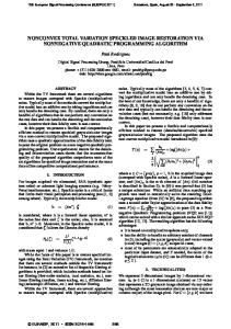
Fig. 1. Convergence profile of PDS, L-ADMM, and Alg. 2 (Prop) on CS reconstruction (left) and non-uniform deblurring (right). analytically unavailable, it was pre-computed by PDS with 100000 iterations. For a fair comparison of stochastic and non-stochastic methods, the convergence curves of the proposed method were obtained after averaging uniformly 100 realizations. 4.1. Compressed sensing reconstruction

min

∥Du∥1,2 s.t. Φu = v.

Blurred

PDS

L-ADMM

b=4

b = 16

b = 64

Fig. 2. Resulting images on CS reconstruction (top) and nonuniform deblurring (bottom). optimization via FFT. In this experiment, a sharp image is restored from a blurred observation v = Φ¯ u + n by solving ∑M ⊤ 2 λ (7) min m=1 (ϕm u − vm ) + ∥Du∥1,2 , 2 u∈[0,255]N

¯ from its In CS reconstruction, we try to recover an original image u incomplete measurements v = Φ¯ u, where Φ is some measurement matrix of size M × N with M < N . Theoretically, employing random matrices as Φ is in some sense an optimal strategy for a stable CS reconstruction [33, 34]. However, such random matrices are dense and have no specific structure allowing efficient implementation, so that the computations of Φx and Φ⊤ y become much expensive and memory inefficient in large-scale problems, as pointed out in [35]. The proposed method provides a resolution to this issue. In this experiment, we solve u∈[0,255]N

Original

(6)

This problem appears different from Prob. (2) because the datafidelity is expressed as the linear constraint Φu = v, but by using M indicator functions ιEm (m = 1, . . . , M ) with Em := {vm }, Prob. (7) can be reduced to Prob. (2) as follows: ∑M ⊤ min m=1 ιEm (ϕm u) + ∥Du∥1,2 . u∈[0,255]N

Since Em is a singleton, the computation of the proximity operator of ιEm (the projection onto Em ) is just replacing the input by vm . For a test image, we used a grayscale Lena image of size 128 × 128 (N = 16384). The measurement matrix Φ was set to a 4096 × 16384 random Gaussian matrix (M = N4 ), i.e., its entries are realizations of i.i.d. random variables from a Gaussian probability density function with mean zero and variance N1 . In this case, all the entries of v is sufficiently decorrelated to each other through the random measurement process, so that we can construct the minibatches by simple partitioning of v. Note that we use a relatively small image because PDS and L-ADMM have to load full Φ at each iteration. The left of Fig. 1 shows the convergence profile of PDS, LADMM, and Alg. 2 on the CS reconstruction experiment. For the proposed method, we tested the three different numbers of minibatches: b = 32, 64, 128. One sees that the proposed method converges much faster than PDS and L-ADMM for all the numbers of mini-batches. The resulting images in Fig. 2 indicate the same PSNR (26.39 [dB]), which illustrates that Alg. 2 properly works. 4.2. Non-uniform deblurring Non-uniform deblurring is a realistic but still challenging problem since the blur kernel is spatially variant, which precludes an efficient

where n is an additive white Gaussian noise with standard deviation σ. The proximity operator of λ2 (· − vm )2 is given by m +x prox λ (·−vm )2 (x) = λv1+λ . 2 For a test image, we used a color Castle image taken from [36] of size 256 × 256 (N = 2562 × 3). The blur matrix Φ was made from spatially-varying (per-pixel) kernels simulating motion-blur. Since the pixels of a blurred image v are spatially correlated to each other, we tested the two ways of mini-batch construction: (i) simple block partitioning and (ii) the spatially-uniform sampling proposed in Sec. 3.2. The noise standard deviation is set to σ = 2.55, and the parameter of the data-fidelity is chosen as λ = 1000. The right of Fig. 1 plots the convergence behavior of PDS, L-ADMM, and Alg. 2 on the non-uniform deblurring experiment, where the three different numbers of mini-batches: b = 4, 16, 64 are examined for Alg. 2 (for a simple implementation of (ii), we set the number of mini-bathes to be squared numbers). One sees that the proposed method is not much more efficient, even slower in some cases, than PDS and L-ADMM, which is different from the case of the CS reconstruction experiment. This is because the blur matrix Φ is relatively sparse, so that the computational advantage of mini-batch decomposition becomes small compared with the case of the dense CS measurement matrix. Hence in such cases, the number of mini-batches should be reasonably small (but not too small not to spoil the benefit of stochastic optimization). Indeed, the proposed method still outperforms PDS and L-ADMM with b = 4 and 16. We also remark that the use of our mini-batch construction strategy (ii) results in much faster convergence than the use of the trivial way (i), which demonstrates that the proposed strategy is effective for spatially correlated cases. Finally, as in the CS reconstruction experiment, we observe that the deblurred images in Fig. 2 (bottom) indicate the same PSNR (26.12 [dB]). 5. CONCLUDING REMARKS We have proposed an efficient image restoration framework based on stochastic proximal optimization. Since the proposed method does not require the multiplication of Φ and variables at each iteration, it would be a powerful choice when the structure of Φ is complicated. Although we focus on convex optimization situations, the proposed method can be applied to image restoration with nonconvex objectives, if the proximity(-like) operator of each function is computable, e.g., the ℓ0 pseudo-norm. With slight modification, one can also use it for image restoration with separated components, such as a recently proposed cartoon-texture decomposition [37].

6. REFERENCES [1] L. I. Rudin, S. Osher, and E. Fatemi, “Nonlinear total variation based noise removal algorithms,” Phys. D, vol. 60, no. 1-4, pp. 259–268, 1992. [2] P. L. Combettes and J.-C. Pesquet, “Proximal splitting methods in signal processing,” in Fixed-Point Algorithms for Inverse Problems in Science and Engineering, H. H. Bauschke, R. Burachik, P. L. Combettes, V. Elser, D. R. Luke, and H. Wolkowicz, Eds., pp. 185–212. SpringerVerlag, New York, 2011. [3] W. Yin, S. Osher, D. Goldfarb, and J. Darbon, “Bregman iterative algorithm for ℓ1 minimization with applications to compressed sensing,” SIAM J. Imag. Sci., vol. 1, no. 1, pp. 143–168, 2008. [4] Z. Lin, R. Liu, and Z. Su, “Linearized alternating direction method with adaptive penalty for low-rank representation,” in Proc. Adv. Neural Inf. Process. (NIPS), 2011. [5] A. Chambolle and T. Pock, “A first-order primal-dual algorithm for convex problems with applications to imaging,” J. Math. Imaging and Vision, vol. 40, no. 1, pp. 120–145, 2010. [6] L. Condat, “A primal-dual splitting method for convex optimization involving Lipschitzian, proximable and linear composite terms,” J. Optimization Theory and Applications, 2013. [7] P. L. Combettes and J.-C. Pesquet, “Primal-dual splitting algorithm for solving inclusions with mixtures of composite, Lipschitzian, and parallel-sum type monotone operators,” Set-Valued and Variational Analysis, vol. 20, no. 2, pp. 307–330, 2012. [8] M. Hirsch, C. J. Schuler, S. Harmeling, and B. Scholkopf, “Fast removal of non-uniform camera shake,” in Proc. IEEE Int. Conf. Comput. Vis. (ICCV), 2011. [9] O. Whyte, J. Sivic, A. Zisserman, and J. Ponce, “Non-uniform deblurring for shaken images,” Int. J. Comput. Vis., vol. 98, no. 2, pp. 168–186, 2012. [10] L. Xu, S. Zheng, and J. Jia, “Unnatural L0 sparse representation for natural image deblurring,” in Proc. IEEE Conf. Comput. Vis. Pattern Recognit. (CVPR), 2013. [11] R. G. Baraniuk, “Compressive sensing,” IEEE Signal Process. Magazine, vol. 24, no. 4, 2007. [12] E. Cand`es and M. Wakin, “An introduction to compressive sampling,” IEEE Signal Process. Magazine, vol. 25, no. 2, pp. 21–30, 2008.

[21] P. L. Combettes and J.-C. Pesquet, “A Douglas-Rachford splitting approach to nonsmooth convex variational signal recovery,” IEEE J. Sel. Topics in Signal Process., vol. 1, pp. 564–574, 2007. [22] X. Bresson and T. F. Chan, “Fast dual minimization of the vectorial total variation norm and applications to color image processing,” Inverse Probl. Imag., vol. 2, no. 4, pp. 455–484, 2008. [23] B. Goldluecke, E. Strekalovskiy, and D. Cremers, “The natural vectorial total variation which arises from geometric measure theory,” SIAM J. Imag. Sci., vol. 5, no. 2, pp. 537–563, 2012. [24] S. Ono and I. Yamada, “Decorrelated vectorial total variation,” in Proc. IEEE Conf. Comput. Vis. Pattern Recognit. (CVPR), 2014. [25] E. Cand`es, L. Demanet, D. L. Donoho, and L. Ying, “Fast discrete curvelet transforms,” SIAM J. Multi. Model. Simul., vol. 5, no. 3, pp. 861–899, 2006. [26] G. Gilboa and S. Osher, “Nonlocal linear image regularization and supervised segmentation,” Multiscale Model. Simul., vol. 6, no. 2, pp. 595–630, 2007. [27] A. Danielyan, V. Katkovnik, and K. Egiazarian, “BM3D frames and variational image deblurring,” IEEE Trans. Image Process., vol. 21, no. 4, pp. 1715–1728, 2012. [28] G. Chierchia, N. Pustelnik, B. Pesquet-Popescu, and J.-C. Pesquet, “A nonlocal structure tensor-based approach for multicomponent image recovery problems,” IEEE Trans. Image Process., vol. 23, no. 12, pp. 5531–5544, 2014. [29] J. Mairal, F. Bach, J. Ponce, G. Sapiro, and A. Zisserman, “Non-local sparse models for image restoration,” in Proc. IEEE Int. Conf. Comput. Vis. (ICCV), 2009. [30] D. Zoran and Y. Weiss, “From learning models of natural image patches to whole image restoration,” in Proc. IEEE Int. Conf. Comput. Vis. (ICCV), 2011. [31] H. Ouyang, N. He, L. Tran, and A. Gray, “Stochastic alternating direction method of multipliers,” in Proc. Int. Conf. Mach. Learn. (ICML), 2013. [32] N. Pustelnik, C. Chaux, and J.-C. Pesquet, “Parallel proximal algorithm for image restoration using hybrid regularization,” IEEE Trans. Image Process., vol. 20, no. 9, pp. 2450–2462, 2011. [33] E. Cand`es and T. Tao, “Decoding by linear programming,” IEEE Trans. Inform. Theory, vol. 51, no. 12, pp. 4203–4215, 2005.

[13] T. Suzuki, “Stochastic dual coordinate ascent with alternating direction method of multipliers,” in Proc. Int. Conf. Mach. Learn. (ICML), 2014.

[34] E. Cand`es, J. Romberg, and T. Tao, “Robust uncertainty principles: exact signal reconstruction from highly incomplete frequency information,” IEEE Trans. Inform. Theory, vol. 52, no. 2, pp. 489–509, 2006.

[14] S. Ono, T. Miyata, and I. Kumazawa, “Image restoration by stochastic proximal optimization,” Tech. Rep., IEICE, Mar. 2015.

[35] E. Cand`es and J. Romberg, “Sparsity and incoherence in compressive sampling,” Inverse Problems, vol. 23, no. 3, 2007.

[15] J. J. Moreau, “Fonctions convexes duales et points proximaux dans un espace hilbertien,” C. R. Acad. Sci. Paris Ser. A Math., vol. 255, pp. 2897–2899, 1962.

[36] D. Martin, C. Fowlkes, D. Tal, and J. Malik, “A database of human segmented natural images and its application to evaluating segmentation algorithms and measuring ecological statistics,” in Proc. IEEE Int. Conf. Comput. Vis. (ICCV), 2001.

[16] H. H. Bauschke and P. L. Combettes, Convex analysis and monotone operator theory in Hilbert spaces, Springer, New York, 2011. [17] A. Defazio, F. Bach, and S. Lacoste-Julien, “SAGA: A fast incremental gradient method with support for non-strongly convex composite objectives,” in Proc. Adv. Neural Inf. Process. (NIPS), 2014, pp. 1646– 1654. [18] A. Repetti, E. Chouzenoux, and J.-C. Pesquet, “A random blockcoordinate primal-dual proximal algorithm with application to 3D mesh denoising,” in Proc. IEEE Int. Conf. Acoust., Speech, Signal Process. (ICASSP), 2014. [19] J.-C. Pesquet and A. Repetti, “A class of randomized primal-dual algorithms for distributed optimization,” arXiv preprint arXiv:1406.6404, 2014. [20] M. Pereyra, P. Schniter, E. Chouzenoux, J.-C. Pesquet, J.-Y. Tourneret, A. Hero, and S. McLaughlin, “A survey of stochastic simulation and optimization methods in signal processing,” arXiv preprint arXiv:1505.00273, 2015.

[37] S. Ono, T. Miyata, and I. Yamada, “Cartoon-texture image decomposition using blockwise low-rank texture characterization,” IEEE Trans. Image Process., vol. 23, no. 3, pp. 1128–1142, 2014.