Image Compression of Natural Images Using Artificial Gene Regulatory Networks Martin A. Trefzer

University of York YO10 5DD, York, UK

[email protected]

Tuze Kuyucu

University of York YO10 5DD, York, UK

[email protected] Andy M. Tyrrell

Julian F. Miller

University of York YO10 5DD, York, UK

[email protected]

University of York YO10 5DD, York, UK

[email protected] ABSTRACT A novel approach to image compression using a gene regulatory network (GRN) based artificial developmental system (ADS) is introduced in this paper. The proposed algorithm exploits the fact that series of complex organisms can be represented via a GRN description and the indices of the developmental steps in which they occur. Organisms are interpreted as tiles of an image tile at each developmental step which results in the (re-)construction of an image during the developmental process. It is shown that GRNs are suitable for image compression and achieve a higher compression rate than JPEG when optimised for a particular image. The behaviour of the dynamic system is investigated by visualising the output tile space of the developmental process. Furthermore it is shown that the same GRN has the potential to encode multiple images, each represented by different series of numbers of developmental steps. Example images Lena, Elaine, Mandrill and Aerial01 are taken from the USC Signal and Image Processing Institute database.

Categories and Subject Descriptors H.4 [Information Systems Applications]: Miscellaneous; D.2.8 [Software Engineering]: Metrics—complexity measures, performance measures

General Terms Algorithms

1.

INTRODUCTION

One of the most fascinating properties of biological development is the fact that large, complex organisms are created using the relatively small piece of information that is encoded in the deoxyribonucleic acid (DNA) of a single cell. Once development is initiated, a complex process of gene

activity and regulation takes place that triggers a series of cell actions which, over time, create complex, multicellular organisms [17]. During the organisms lifetime, the developmental process constantly adapts it to changing environments and maintains it in the case of damage [1]. Hence, the crucial factor that allows developmental processes to unfold their power is time. From an engineering and computer science point of view, this means that information is encoded in the time steps of a dynamic system. In this respect, the DNA represents compressed information, which is expanded during the developmental process and is expressed through the various states of the organism. Most of the current research and applications in the area of artificial developmental systems (ADS) concentrate on the properties of development that also help biological organisms to survive and maintain themselves, namely adaptivity, robustness and self repair. In addition to scalability these features are also desirable in engineered systems like embedded systems, robots and control systems [5, 9, 2, 3, 14, 13, 15]. [insert better citations] One of the most prominent applications for studying ADSs in the field of evolutionary computation (EC) and biological modeling is pattern generation and pattern formation [12, 7, 6, 14, 15, 3], which is also the inspiration for the algorithm introduced in this paper. In most of the work, a two-dimensional array of identical entities (cells) is used to achieve a 2D pattern which is defined through the cell states or protein concentrations. There are also examples where development takes place in three dimensions and examples where the cells have different shapes and can migrate. Questions which are addressed in pattern formation experiments include growth, symmetry, shaping, stability and recovery from damage[references]. Unlike in most of the work on pattern formation, where the aim is to achieve a certain pattern or shape and maintain it indefinitely, the idea behind this work is to optimise a GRN in a manner that it matches patterns of a given set of target patterns as closely as possible at arbitrary developmental steps and use it for image compression: for a defined starting point, the developed organisms can be enumerated according to the order in which they occur while running the ADS. Hence, a sequence of complex states can be rep-

resented by the GRN and a sequence of integers. If the pattern at each developmental step is interpreted as tile of a larger image, the image will be (re-)constructed during the developmental process. From a data compression point of view this is ideal since the states can become arbitrarily complex while the amount of compressed data remains constant for a fixed number of developmental steps. However, there are two major issues that render this kind of data compression impractical: first, the optimisation of the dynamic system is NP-hard, hence, is time consuming and requires a large amount of computation. Second, it is not necessarily guaranteed that an arbitrary set of data can be exactly matched by any implementation of an ADS. While dynamic systems are probably not practical for lossless data compression, this work investigates the application of GRNs to lossy image data compression. In the latter case, it is not necessary to encode a perfect version of the input data, as long as sufficient image quality is achieved. In cases where smaller amounts of data are more important than maximum quality, the compression rate can be increased at the cost of losing information, i.e. losing image detail.

The quantisation matrix is the same for all tiles and predefined. Again, the fact that the human eye is less sensitive to small localised variations in colour or brightness (small details) is exploited by storing the high frequency components with a lower accuracy. The lower the quality setting, the more of the high-frequency components are completely discarded. Finally, the resulting data is compressed using a lossless entropy encoder, i.e. Huffman encoding. In order to decode the image these steps are preformed in reverse order. Quantisation is reversed by multiplying each component with the corresponding entry of the quantisation matrix, which is stored within the JPEG file. Quantisation in JPEG is the reason why it is a lossy compression method, where the amount of data lost is determined by the values of the matrix elements of the quantisation matrix. For the DCT exists an inverse transformation (DCT−1 ), which is used to convert back to the time domain.

2.2

Vector Quantisation

Joint Photographic Experts Group (JPEG) image compression and image compression via vector quantisation (VQ) are relevant for the proposed image compression algorithm and the results presented. JPEG compression is chosen as a benchmark for the reason that JPEG is a widely adopted image compression standard for natural images. Hence, the assessment of the proposed algorithm can be based on a method which is established and optimised.

Image compression via VQ is based on the idea that a series of input vectors, which correspond to parts of the original image, can be represented by an index that points to the closest match within a minimised codebook, thereby reducing the amount of data that needs to be stored. At the encoding (compression) stage, each input vector is matched against a codebook and represented by the index of the codeword with the smallest euclidean distance to the input. At the decoding (decompression) stage, the original data is reconstructed by combining the codewords from the codebook according to a sequence of indices. The smaller the size of the codebook the higher the compression rate at the cost of increased data loss. In the case of the proposed method, the codebook is represented by the GRN which creates the codewords during the developmental process. This has the advantage that the ’codebook’ does not change in size when generating a larger number of tiles, since development could simply be run for longer, exploiting the fact that information is encoded in time, rather than additional code words. In VQ there are several algorithms to find and optimise the codebook, for instance, pairwise nearest neighbour (PNN), simulated annealing, maximum descent (MD), and frequencysensitive competitive learning (FSCL) and Linde-Buzo-Gray (LBG)[references!]. Like optimising a DS, finding the optimal codebook is an NP-hard problem and may take a long time when high quality is required, which is the reason why VQ is not more widely used.

2.1

3.

The results in this paper show that GRNs are suitable for image compression and achieve a higher compression rate than JPEG when optimised for a particular image. The behaviour of the dynamic system is investigated by visualising the output tile space of the developmental process, which provides insight on how the ADS explores the feature space of the image. Furthermore it is shown that the same GRN has the potential to encode multiple images, each represented by different series of numbers of developmental steps. Example images Lena, Elaine, Mandrill and Aerial01 are taken from the USC Signal and Image Processing Institute database. Images which are encoded using the proposed algorithm are denoted as Gene Compressed Image (GCI), which is also proposed as the name and file extension for the image format.

2.

IMAGE COMPRESSION

JPEG Image Compression Standard

JPEG is a lossy image compression algorithm. The encoding process encompasses the following steps: first, the colour space of the image is converted into YCbCr, where Y is the luma component—which effectively represents an 8bit grey scale version of the image—and Cb and Cr represent the colours. Second, the resolution of the colour channels is reduced, usually by a factor 2. This is called sub-sampling and accounts for the fact that the human eye has a lower resolution for colour than for brightness. Third, the image is split into tiles of 8×8 pixels. Each of those tiles is converted to the frequency domain using a two-dimensional discrete cosine transform (DCT). The fifth step achieves the actual data reduction (quantisation), by dividing each of the amplitude values by the corresponding value in a quantisation matrix.

THE DEVELOPMENTAL SYSTEM

The GRN based model for artificial development used in this paper is based on the one that has been introduced in[16, 10]. The design considerations of the original ADS are retained, namely the usage of data structures and operations in the GRN core that are suitable for embedded systems, i.e. boolean, integers, no division and to keep the mechanisms of the ADS as close as possible to their biological counterparts within the boundaries of the chosen data types. Whilst not crucial for the experiments in this paper, the choice of the data structures imposes no loss of generality and is therefore unchanged. However, some improvements are made to the ADS for this paper: first, a dedicated diffusion layer is added and only chemicals that are released to this layer by the cells are subject to diffusion. Chemicals need to be absorbed by

Algorithm 1 The function of the structuring protein is given in pseudo-code. Structuring gene actions express pixel values or frequency components of a rectangular image area. When a gene is expressed, the functions of all of its structuring proteins are carried out and modify the cell type (=current pixel value/frequency component).

Proteins from Neighbouring Cells Environment Inputs

Sensor Protein

Regulatory Feedback

Messenger Molecule

DNA Sequence

Transcription

Cell Output Functions Protein

Bd:AAD>
Regulatory Elements (Precondition) Gene Action (Postcondition)

par1 , par2 = parameters of structuring protein ctype = cell type (pixel value, freq. component) nchem = total no of protein and molecule types chem = protein or molecule type lev(chem) = chemical level chem ← par2 mod #chem switch par2 ≡ 0(mod 16) case 0 : ctype = lev(chem) case 1 : ctype = -lev(chem) case 2 : ctype = -ctype case 3 : ctype = lev(chem)-lev((chem+1) mod nchem ) case 4 : ctype = lev(chem)-lev((chem+2) mod nchem ) case 5 : ctype = lev(chem)-lev((chem+3) mod nchem ) case 6 : ctype = lev((chem+1) mod nchem )-lev(chem) case 7 : ctype = lev((chem+2) mod nchem )-lev(chem) case 8 : ctype = lev((chem+3) mod nchem )-lev(chem) case 9 : ctype = ctype+7; case 10 : ctype = ctype-7; case 11 : ctype = ctype+4; case 12 : ctype = ctype-4; case 13 : ctype = ctype+1; case 14 : ctype = ctype-1; case 15 : ctype = ctype; end switch

the cells from the diffusion layer first, before they affect gene regulation. This is motivated by natural development. Second, a genetic representation that allows for variable length GRNs is used in this paper, which allows for a more flexible and compact encoding of the genes 2. An overview of the mechanisms of the ADS is provided in the following sections. The term chemicals refers to both proteins and molecules.

3.1

Representation and Gene Regulation

The core of the developmental model is represented by a GRN, as shown in figure 1. The DNA is implemented as a string of symbols that encode start and end of genes, separation of pre- and postcondition within genes, binding sites and chemicals as shown in figure 2. Genes interact through chemicals and form a regulatory network. The major difference between the artificial model and biology is that in this case the binding sites match exactly one chemical, whereas in natural genes binding sites are defined by certain upstream and downstream gene sequences that accept a number of proteins to bind and transcribe their genetic code. The binding sites in natural DNA therefore allow for smooth binding, i.e. the probability that certain chemicals (transcription factors) bind to the DNA is given by how well the binding sites of the chemical matches the one of the DNA. There are examples of artificial GRNs where soft-binding is included [8, 4]. However, it is not clear whether including soft-binding yields major benefits and the inclusion of this feature is extremely expensive in terms of memory require-

Figure 1: The genes in a DNA sequence are activated when a sufficient amount of protein is produced by the GRN, which then causes transcription of the respective gene. In the example shown in the figure, the activity of the GRN results in the correct transcription factors (the promoter proteins) that bind to the sites of a gene sequence. This initiates the production of another protein, which can then affect the cell functionality using further information that is encoded in the gene. The produced protein also provides feedback to the GRN, which regulates the transcription of further genes, hence, dynamic gene regulation is achieved. Note that when any inhibitory condition is met, the gene is not expressed. ment and computation effort. In principle the ADS used can work with an arbitrary number of chemicals. However, the current system is working with eight chemicals: four proteins and four molecules. Gene regulation is described in figure 2. A description of the proteins and their roles is given in table 1. The total number of chemicals is arbitrarily chosen. Increasing the number of chemicals increases the complexity of the dynamics of ADS, but makes it slower to process. The presence of molecules, which cannot be directly produced by the GRN, motivated by natural development where they play a significant role in gene regulation [17].

3.2

Evolution of the DNA

The DNA is derived from a genome that is evolved using a standard 1 + 4 evolutionary strategy (ES). The EA parameters are based on values that are widely used in the field of evolutionary computation (EC)[references]. The genome is represented by a string of integers and mutation takes place by replacing them with a new random value at a rate of 2% of the genome length. Crossover is not used. The GRN is obtained by mapping the string of integers to GRN symbols using the modulus operation on the genome in a straight forward fashion. Variable length genes are achieved via active/inactive flags encoded in the genes.

3.3

Cell Communication and Growth

Wolpert [17] describes three different types of cell signalling: chemical diffusion, direct contact of complementary chemicals on the cell’s surface, and gap junctions (Plasmodesmata). Two different types of cell signalling are realised in the proposed model. Chemical diffusion has been implemented in a similar way as it takes place in physical systems, e.g. a drop of ink dissolving in water. Half of the cells chemical is thereby distributed amongst its nearest neighbours in equal shares, i.e. each neighbour obtains 81 of the cell’s chemical. Chemical levels are credited and debited after the GRN has processed the next developmental step for all

GRN DNA ....< Gene >< Gene >< Gene >< Gene >..... < Precondition : Postcondition >

Proteins elem. {A,B,C,D,...} Molecules elem. {a,b,c,d,...}

Protein/ Molecule, Production Rate, 2 Function Parameters Protein, Threshold, Bindingsite Type, Protein Consumption Rate

Figure 2: An example DNA is shown in the figure above. The GRN comprises a number of genes that are separated by brackets. A gene consists of pre- and postcondition, which are separated by a colon. Each letter refers to one type of protein or molecule and is parametrised by three integer parameters. Both proteins and molecules are present in the gene’s precondition and contribute to gene regulation whereas only proteins can be directly produced in the postcondition. In the case of precondition, the letter defines which type of chemical can bind to this site. The parameters are then interpreted as the protein threshold that is necessary to activate the binding site, the type of binding site (inhibitory or excitatory), and the rate at which the binding protein is consumed while the site is active. In the case of postcondition, the parameters are interpreted as the production rate of the respective protein and as parameters for the respective protein function. An overview of the protein functions is shown in table 1.

cells. Thus, the GRN always works with the original chemical levels and the order of cell update should therefore not bias the course of development. Diffusion only takes place on a separate diffusion layer which is underlying the array of cells (organism). Only chemicals that are released by a cell via the according cell action participate in the diffusion process. Vice versa cells can absorb chemicals from the diffusion layer, which only then affect gene regulation within the respective cell. Diffusion is a signalling mechanism that helps maintaining symmetries within the system. The second cell signalling mechanism is an implementation of Plasmodesmata in plants (protein tunnels) [11]. The GRN produces a Plasmodesmata protein for one of the four directions N,S,E,W. If the neighbour cell is alive and produces the complementary Plasmodesmata protein, a tunnel will be established between the two cells with the effect that all chemicals are equally shared between those cells, as depicted in figure 3. This tunnel is active as long as the necessary Plasmodesmata proteins are produced. Complementary to diffusion, the tunnelling mechanism should enable the GRN to break symmetries within the system, due to the fact that tunnels do not necessarily occur on all four sides of the cell at the same time. Cell growth is achieved using the Plasmodesmata proteins. If the neighbour cell, which is targeted by the tunnel, is an empty or dead cell, it will become alive during the next developmental step (see figure 3). Cell death is not imple-

Table 1: The current GRN works with four proteins and four molecules. Proteins are directly produced by the GRN, whereas molecules are only product of a gene function as a result of a measurement or interaction that is performed by a protein. Their roles in development are described in the table. Please note that all proteins and messenger molecules take part in gene regulation, in addition to their special purpose. Protein/ Role (apart from gene regulation) Molecule

Structuring (Protein A)

Structuring proteins are used to alter the cell state according to a set of predefined rules. In this paper, the cell state represents a pixel value in the time-domain or a coefficient in the frequency-domain. The structuring function is described in Algorithm 1.

Sensory/ Interacting (Protein B)

Sensory proteins provide a means to react to changes in the cell state. Molecules are produced, based on the current cell function, cell location and possible rules that can be encoded in the genes.

Diffusion Layer (Protein C)

Diffusion layer proteins release chemicals to the diffusion layer and absorb them from the diffusion layer. Only chemicals which are released to the diffusion layer are subject to the diffusion process. Chemicals on the diffusion layer need to be absorbed by the cell first, before they affect gene regulation.

Plasmodesma (Protein D)

Plasmodesma proteins provide a mechanism to form Plasmodesmata [11] in order to share their proteins with neighbour cells, and they initiate growth.

Molecules (a,b,c,d)

Molecules are produced as a result of the sensor protein being expressed and reacting according to the current cell state or environment input.

mented at the current stage. The cells are surrounded by border cells, which absorb any amount of chemical that diffuses outwards on the diffusion layer. Since the border cells are inactive, i.e. not processed by the GRN, they are unable to produce chemicals and form tunnels. Hence, tunneling outside the bounds of the organism is impossible.

3.4

Developing Organisms to Form Images

The application in this paper is image compression via GRN. Therefore, the GRN has to be able to represent an image or parts of an image. This is achieved by designing the function of the structuring protein in such a manner that it can represent positive and negative integer values via the cell state. It is then possible to interpret the states of a rectangular area of cells as a corresponding area of pixel values where one cell represents one pixel. In the time domain it would be sufficient to cover a value range of 0 . . . 255 in order to represent

Cell In1

Physical Cell  Structure

Sensors Cell In2

A complete  Plasmodesma

GRN Core

Cell In3

Plasmodesma Proteins

CELL 2 An incomplete Plasmodesma

Structuring Proteins

CELL 1

Cell Out

New Cell CELL 3

Figure 3: In a multi-cellular environment using the four protein types from Table 1 a cell is able to: interact with its environment, multiply, represent a pixel value or frequency component, and form a complex multicellular organism.

an 8bit grey-scale image. However, for many image processing applications it is more beneficial to represent images in the frequency domain using DCT or Fourier transformation. In both cases the rectangular array of pixel values becomes an array of coefficients for two-dimensional frequency components of the image. Usually, the upper left element represents the DC coefficient and the frequency increases towards the lower right coefficient. The coefficients can take on relatively large positive and negative values (±800 in the case of Lena). Hence the value range of the cell state has to be wider than 0 . . . 255 and also cover negative values. The implementation of the functions of the structuring protein is described using pseudo-code in Algorithm 1.

4.

IMAGE COMPRESSION USING GRN

The presented image compression algorithm is based on the idea of replacing 8×8 pixel tiles (64 bytes in the time domain or 64 integers in the frequency domain) of an image with a single integer value in order to achieve data compression. This is similar to VQ 2.2, where input tiles of an image are represented by the index of a tile from a codebook that offers the least distortion. Hence, in order to restore the image, only the codebook and the array of indices obtained from encoding the input vectors need to be saved. The smaller the codebook is compared to the input space, the greater is the data reduction but also the loss of information. In this paper a GRN based ADS is used, which is able to produce a series of 8 × 8 cell organisms during the developmental process. For encoding, an EA is used to optimise the GRN to produce organisms that are able to represent the 8 × 8 pixel tiles of an image in such a way that for each one the distortion is minimised at an arbitrary developmental step. As a consequence, the encoded image consists of the GRN and the iteration numbers of the developmental process where the closest matches of the input tiles occur. In this respect the GRN and iteration numbers work similar to the codebook and indices in VQ. In order to decode an image, the developmental process is (re-)run using the optimised GRN, which reproduces the series of 8 × 8 cell organisms (image tiles). The image is then restored by ar-

Algorithm 2 GRN based image encoding (compression) and decoding (decompression) is described in pseudo-code. Multi-pass encoding can be achieved by repeatedly running the encoder and decoder. The term GCI file refers to genetically compressed image (GCI) files. Encoder: 1. Divide input image into a set of 8 × 8 tiles 2. Convert tiles to frequency domain using DCT {optional} 3. Optimise GRN to produce a stream of organisms (tiles) with minimum distortion to the input tiles via EA 4. Initialise development: Initialise all chemical levels to 0 Initialise 8 × 8 cells organism Set cell(1,1) alive 5. During development: Record iteration numbers of organisms with minimum distortion to input tiles 6. Save GRN and iteration numbers to GCI file 7. Use bzip2 for entropy encoding of GCI file Decoder: 1. Load and unzip GCI file 2. Initialise development as in Encoder 3. Run loaded GRN 4. During development: When iteration number matches one from the GCI file replace it with the current organism 5. Convert tiles to time domain using DCT−1 {if done for encoding} 6. Reconstruct image Multi-pass: 1. Subtract the resulting image tiles from the ones of the original image (or the previous pass) 2. Run the Encoder on the resulting tiles 3. For decding, run the Decoder using the iteration numbers and GRNs form each pass separately 4. Add up all resulting sets of tiles and reconstruct the image

ranging tiles according to the sequence of iteration numbers. Since the optimisation of the GRN is an NP-hard problem, the encoding process is time consuming (2-3 days for high quality), whereas the decoding process is fast (seconds). The compression algorithm is described in Algorithm 2. It is further possible to perform multi-pass encoding on the input image, which results in a larger GCI file since for each pass another GRN and set of iteration numbers needs to be stored. However, as shown in the results, multi-pass encoding can do both speeding up encoding and achieve higher quality of the compressed images. A tile size of 8 × 8 pixels of grey-scaled images is used for the following reasons: first, 8 × 8 pixel tiles are widely used in image compression algorithms, particularly in JPEG[references], against which the presented results are compared. Second, one pixel corresponds to one cell in the current implementation and it is easier to achieve smaller organisms that match smaller tiles.

PSNR (Image Quality) [dB]

50

JPEG GCI

45 40

(a) JPG qual. 10% (b) JPG qual. 50% (c) JPG qual. 90%

35 30 250.0

0.5

1.0

1.5

2.0

Bits Per Pixels [BBP]

2.5

3.0

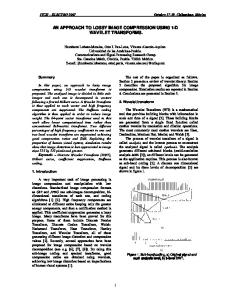
Figure 4: A comparison between JPEG and GCI is shown. A higher PSNR value reflects a better image quality whereas a lower BBP value means higher compression. In the case of JPEG the best quality shown using a JPEG quality setting of 95% achieves a PSNR of 45dB. As can be seen from the graph a higher compression rate is achieved for the same PSNR using GCI 6-pass encoding.

5.

GENE COMPRESSED IMAGE VS JPEG

In the first experiment it is investigated what quality and compression rates are achievable when compressing images with the proposed method (Algorithm 2). Bits per pixel (BPP) is a measure for image compression and has a value of 8 for 8bit grey scale, uncompressed images. In this paper the BBP value is simply calculated by dividing the resulting image file size by the total number of pixels. The quality of the compressed image is measured by calculating its peak signal-to-noise ratio (PSNR) to the uncompressed image. Results are compared with JPEG in order to place them into the context of an established and optimised method. The example image Lena is taken from the USC Signal and Image Processing Institute database[ref!]. The original version is a 512×512 pixel, uncompressed, 8bit grey scale image in Tagged Image File Format (TIFF), hence, the image consists of 4096 8 × 8 pixel tiles. The number of iterations of the ADS is set to 4096, which is the minimum when assuming each tile is different, since multi-pass encoding is used and in order to keep computation time low. Results for multi-pass encoded GCI images (1. . . 6 passes) are compared with JPEG images that are encoded with quality settings of 5, 10, 20, . . . , 90, 95% in figure 4. As can be seen from figure 4, applying multiple passes in GCI correspond to increasing the quality setting in JPEG. BBP and PSNR is calculated as described above for both GCI and JPEG images. Figure 5 shows example images for both methods using the lowest and the highest quality setting respectively.

6.

DYNAMICS OF THE GRN

In order to investigate the dynamic behaviour of the GRN, the tiles of every developmental step are recorded and the resulting 4096 tiles are arranged in a square as shown in Figure 6. As examples, the tile spaces sampled by the GRNs

(d) GCI 1-pass

(e) GCI 4-passes

(f) GCI 6-passes

Figure 5: Comparison of JPG and GCI at low, medium and high quality settings. of encoding pass 1 and 2 are shown. As can be seen from Figures 6(a) and 6(b), only a relatively small part of the output tile space of pass 1 is used to represent the image. It is observed in Figure 6(b) that mostly tiles from early iterations of the developmental process are used. The reason for this is the fact that the GRN is optimised to create tiles in frequency space, which emphasises the DC value of the tile and the lower frequency components when calculating the fitness as those feature the largest coefficients. Once the brightness of all tiles in the image is matched by producing basic tiles representing all 128 grey levels, the system is in a local optimum. This behaviour is the main reason for using multi-pass encoding in order to increase image quality. In later encoding passes the emphasis is shifted towards higher frequency components due to the fact that only the differences to the tiles that are already produced in earlier passes need to be achieved. An example of this is shown in Figures 6(c) and 6(d), where the target image and the output tile space of pass 2 is shown. In this case, a larger part of the tile space is contributing to creating the image and the tiles used are not clustered at early developmental steps. However, using multi-pass encoding to increase image quality comes at the cost of increasing the file size of the GCI image, since, for each pass a new GRN, it’s parameters and the sequence of integers to identify the tiles needs to be stored. This suggests that there is scope for improvement of the dynamic system in order to exploit the entire tile space.

7.

GENERALITY OF GCI

The results from Section 6 suggest that it should be possible to encode more than one image, particularly if they contain similar features, using the same set of GRNs. Theoretically, the output tile spaces of the 6 encoding passes used to encode Lena can be linearly combined to represent 40966 different 8 × 8 image tiles, which can be used to form a variety of different images. It is investigated whether it is possible to encode three images other than Lena, which are

(a) Tile space pass 1

(b) Tiles used pass 1

PSNR (Image Quality) [dB]

50 45 40

Lena Elaine Ape Aerial

35 30 25 20 150.0

0.2

0.4

0.6

0.8

1.0

Bits Per Pixels [BBP]

1.2

1.4

Figure 7: PSNR of different images using multiple passes of GCI encoding. For comparison, results for JPEG of the highest quality achieved by GCI are included and marked with a circle. (c) Tile space pass 2

(d) Tiles used pass 2

Figure 6: Output streams of the 4096 tiles produced by the GRN of pass 1 and 2. also taken from the USC Signal and Image Processing Institute database[ref!], namely Elaine,Mandrill and Aerial01. The same set of GRNs that is originally optimised for Lena is used to encode these images. Results of the GCI encoded versions of the three images are shown in Figure 8. The original size of the images is 512x512 pixels, hence, compression artefacts are only visible in the magnified versions that only show a part of the image. The results show that it is possible to encode different images using the same set of GRNs. However, as can be seen from Figure 7, quality and compression rate of the GCI encoded versions of Elaine,Mandrill and Aerial01 are lower than in the case of Lena, for which the set of GRNs is optimised. As one might expect, the Elaine image, which is most similar to Lena, achieves the best PSNR and BBP of the three. GCI encoding performs worse on the Mandrill and Aerial01 due to greater level and characteristics of detail in those images.

8.

DISCUSSION

A novel approach to image compression is proposed in this paper. It is shown that GRN based artificial developmental systems are suitable for image compression and outperform JPEG when optimised for a particular image. In the case of Lena, the compression rate is increased by a factor of 2.5 at the highest quality setting. The behaviour of the ADS is investigated by visualising the output tile space of the developmental process. This provides insight into the way GCI works and reveals an important bias of the current implementation towards lower frequencies in early encoding passes. This bias is present due to the fact that the ADS is optimised to match tiles in frequency space, which puts more emphasis on the usually

(d) Elaine

(e) Ape

(f) Aerial

Figure 8: Encoding different images with the same set of GRNs. The bottom row shows details of the images in the top row.

larger coefficients of the lower frequency components. This could be taken into account when improving the function of the structuring protein (1) in future experiments. When working in frequency space, for instance, it might be beneficial to make this function dependent on the position of the cell within the 8 organism. Furthermore it is shown that the set of GRNs, which is originally optimised for encoding Lena, is suitable to encode a variety of other natural images as well. As expected, the experiments undertaken show that the more similar features and characteristics to Lena are present in the image to encode, the better GCI compression performs both in terms of visual inspection and PSNR. When encoding ’unknown’ images the higher compression rate than JPEG is generally not achieved, although if the goal is to encode a variety of different images, it will be beneficial to include a mixture of tiles from different images for the optimisation of the ADS.

There is also scope for future research on using ADSs for image compression: for instance, an interesting question is whether it is possible to reduce the number of encoding passes and thereby further increase the compression rate. Possible ways of achieving this could be by introducing structural feedback (schedules) in the developmental process which can help to overcome the bias towards lower frequencies or multi-pass encoding could be achieved by introducing multiorganism artificial developmental system. One of the major drawbacks of the proposed approach is at the moment that it takes a lot of time and computational effort to optimise the GRN. However, there are scenarios where higher data compression is more critical than computational effort. Examples for such scenarios are remote applications, i.e. space applications where communication windows are physically limited, and robot applications where the amount of memory is limited. In the latter scenarios, the GRN could be optimised at the base station for images (or other sensor data) of the environment encountered by the field units, which would increase the data compression for transmission over time. Updated versions of the GRN can be transmitted at low cost, as they can be represented in a compact fashion and running the ADS is computationally cheap (the version in this paper already uses exclusively integer data structures and no multiplication or division), as opposed to optimising the system via an EA. Another beneficiary of the image compression application presented in this paper could be the research field of artificial developmental systems, where a lot of work concentrates on pattern formation. The proposed algorithm could be suitable as a benchmark application for ADSs, which would be of more complex nature than achieving static patterns or shapes and would also put less constraints on the way the ADS explores the state space, since the order in which solutions are developed is not important.

9.

REFERENCES

[1] J. T. Bonner. The origins of multicellularity. Integrative Biology: Issues, News, and Reviews, 1(1):27–36, 1998. [2] K. Clegg, S. Stepney, and T. Clarke. Using feedback to regulate gene expression in a developmental control architecture. In Proceedings of Genetic and Evolutionary Computation Conference (GECCO) 2007, pages 966–973, New York, NY, USA, 2007. ACM. [3] A. Devert, N. Bredeche, and M. Schoenauer. Robust multi-cellular developmental design. In GECCO ’07: Proceedings of the 9th annual conference on Genetic and evolutionary computation, pages 982–989, New York, NY, USA, 2007. ACM. [4] N. Flann, J. Hu, M. Bansal, V. Patel, and G. Podgorski. Biological development of cell patterns: Characterizing the space of cell chemistry genetic regulatory networks. In Proceedings of Advances in Artificial Life, 8th European Conference, ECAL 2005, volume 3630 of Lecture Notes in Computer Science, pages 57–66, Canterbury, UK, September 2005. Springer. [5] T. G. W. Gordon. Exploiting Development to Enhance the Scalability of Hardware Evolution. PhD thesis,

University College London, July 2005. [6] P. C. Haddow, G. Tufte, and P. van Remortel. Shrinking the genotype: L-systems for EHW? In ICES, pages 128–139, 2001. [7] G. S. Hornby. Generative representations for evolving families of designs. In Genetic and Evolutionary ˘ S GECCO-2003, volume 2724 of Computation a ˆA¸ LNCS, pages 1678–1689. Springer-Verlag, 2003. [8] J. F. Knabe, C. L. Nehaniv, and M. J. Schilstra. Regulation of Gene Regulation - Smooth Binding with Dynamic Affinity affects Evolvability. In IEEE Congress on Evolutionary Computation (CEC 2008). Proc WCCI 2008, pages 890–896. IEEE Press, 2008. [9] S. Kumar and P. Bentley, editors. On Growth, Form and Computers. Elsevier Academic Press, 2003. [10] T. Kuyucu, M. Trefzer, J. F. Miller, and A. M. Tyrrell. On the properties of artificial development and its use in evolvable hardware. In IEEE Symposium Series on Computational Intelligence - IEEE SSCI 2009, 2009. [11] O. Leyser and S. Day. Mechanisms in Plant Development. Blackwell, 2003. [12] A. Lindenmayer. Mathematical models for cellular interactions in development. i. filaments with one-sided inputs. Journal of Theoretical Biology, pages 280–299, 1968. [13] H. Liu, J. F. Miller, and A. M. Tyrrell. Intrinsic evolvable hardware implementation of a robust biological development model for digital systems. In EH ’05: Proceedings of the 2005 NASA/DoD Conference on Evolvable Hardware, pages 87–92, Washington, DC, USA, 2005. IEEE Computer Society. [14] J. F. Miller. Evolving developmental programs for adaptation, morphogenesis, and self-repair. In 7th European Conference on Artificial Life, pages 256–265. Springer LNAI, 2003. [15] D. Roggen. Multi-Cellular Reconfigurable Circuits: Evolution Morphogenesis and Learning. PhD thesis, EPFL, 2005. [16] M. Trefzer, T. Kuyucu, J. F. Miller, and A. M. Tyrrell. A model for intrinsic arti¨ıˇ nAcial development , featuring structural feedback and emergent growth. In IEEE Congress on Evolutionary Computation, 2009. [17] L. Wolpert, R. Beddington, T. Jessel, P. Lawrence, E. Meyerowitz, and J. Smith. Principles of Development. Oxford University Press Inc., New York, 2 edition, 2002.