Identifying Users’ Topical Tasks in Web Search Wen Hua†‡∗ Yangqiu Song‡ Haixun Wang‡ Xiaofang Zhou§† † Renmin University of China, Beijing, China ‡ Microsoft Research Asia, Beijing, China § University of Queensland, Brisbane, Australia
[email protected] {yangqiu.song, haixun.wang}@microsoft.com
[email protected]
ABSTRACT A search task represents an atomic information need of a user in web search. Tasks consist of queries and their reformulations, and identifying tasks is important for search engines since they provide valuable information for determining user satisfaction with search results, predicting user search intent, and suggesting queries to the user. Traditional approaches to identifying tasks exploit either temporal or lexical features of queries. However, many query refinements are topical, which means that a query and its refinements may not be similar on the lexical level. Furthermore, multiple tasks in the same search session may interleave, which means we cannot simply order the searches by their timestamps and divide the session into multiple tasks. Thus, in order to identify tasks correctly, we need to be able to compare two queries at the semantic level. In this paper, we use a knowledgebase known as Probase to infer the conceptual meanings of queries, and automatically identify the topical query refinements in the tasks. Experimental results on real search log data demonstrate that Probase can indeed help estimate the topical affinity between queries, and thus enable us to merge queries that are topically related but dissimilar at the lexical level.
Categories and Subject Descriptors H.3.3 [Information Storage and Retrieval]: Information Search and Retrieval—Clustering, Query formulation, Search process
General Terms Algorithms, Design, Experimentation, Performance
Keywords Task Identification, Probase, Conceptualization, Interleaved Task
1. INTRODUCTION A search task consists of a query and its refinements for accomplishing a specific information need. A recent study [13] suggests ∗
The work is done at MSRA, Beijing, China.
Permission to make digital or hard copies of all or part of this work for personal or classroom use is granted without fee provided that copies are not made or distributed for profit or commercial advantage and that copies bear this notice and the full citation on the first page. To copy otherwise, to republish, to post on servers or to redistribute to lists, requires prior specific permission and/or a fee. WSDM’13, February 4–8, 2013, Rome, Italy. Copyright 2013 ACM 978-1-4503-1869-3/13/02 ...$15.00.
that tasks are better information units than single queries or sessions1 for many web search applications such as query suggestion, determination of user satisfaction with search results and prediction of user search intent, to name a few. Consider for example, query suggestion. In Web search, query suggestion uses click data to recommend queries that are co-clicked with the original query. Given a query “flight to LA”, we may recommend a query “cheap US flight”. However, queries such as “hotel in LA”, which do not have co-clicks with the original query, are also relevant because they also belong to the task of planning a trip to Los Angeles. In order to be able to recommend such queries, we can extend single-querybased query suggestion to session-based query suggestion. That is, we leverage the co-occurrence frequency of queries in search sessions for recommendation. However, a session may contain queries with multiple user intents, so if we treat queries in a session indiscriminately, we may recommend queries that are not related to the original query. Tasks, on the contrary, represent atomic information needs, which means that queries contained in the same task are usually related. Therefore, tasks can serve as better units for query suggestions, and thus help improve user search experience. However, task identification itself is far from simple, due to the following reasons: First, it is not trivial to decide whether two queries belong to the same task. A real task may contain queries on the same topic but have no lexical similarity, e.g., similarity on the bag-of-words level. For example, queries 4, 5, and 6 in Table 1 may belong to the same task, as “cat”, “dog” and “snake” may be of the same topic (“animal”), although the three queries share little bag-of-words similarity. Therefore, we need a semantic mechanism to identify topical query refinements. Second, inferring semantics from a query or a short piece of text is a complex task. Lucchese et. al. [14] address this problem by simply mapping each word in a query to a set of Wikipedia articles that contain the word. Then, the “meaning” of a query is represented by the combination of the Wikipedia articles that correspond to each word in the query. However, we may not be able to derive topics from single words. For example, when the query “tiger woods” is split into two words, namely “tiger” and “woods”, the concepts related to “animal” and “material” will then be retrieved, instead of “athlete”. Additionally, many words are ambiguous. Consider for example, the word “python” in Table 1. It may refer to a snake or a programming language. Consequently, the problem of detecting topical query refinements becomes much more challenging, due to the existence of ambiguity. Third, tasks in one session may interleave (e.g., task 1 and 2 in Table 1). Previous attempts ignore this phenomenon and identify task boundaries using a Sequential Cut 1 In this paper, we use session to denote a sequence of queries issued within a fixed period of time, or queries issued on a particular web browser as long as the user does not close the browser.
algorithm. Recently, Jones and Klinkner [11] use a Graph Cut algorithm to merge every pair of similar queries into one task. This approach, which is obviously more accurate, also introduces two issues: 1) it is computationally costly; and 2) it may lead to the problem of “over-merging”. For instance, consider the query “the rain song youtube” in Table 1. It contains two concepts, i.e., “song” and “video site”, but its real intent is to find a “song”. Similar for query “the largest dog youtube”. If we calculate the similarity of each pair of queries based on their common concepts, which is the process used in Graph Cut, the two queries mentioned above will be regarded as similar and grouped together. The problem also exists in Sequential Cut, but it becomes more obvious in Graph Cut, as every pair of queries is considered. Therefore, we need to merge queries in interleaved tasks efficiently without over-merging. This requires us to detect concepts that truly reflect users’ search intent. QUERYID 0 1 2 3 4 5 6 7 8
QUERY the rain song youtube cool math the ugliest cat in the world the cutest cat in the world the tiniest cat in the world the largest dog youtube the largest snake on the earth python wikipedia cool math for kids
TASKID 0 1 2 2 2 2 2 2 1
Table 1: An example of tasks in one session. In this work, we build a conceptualization mechanism based on an external knowledgebase (Probase [17]) to infer the underlying conceptual meanings of queries and reduce query ambiguity. We also employ a Sequential Cut and Merge (SCM) algorithm to address the problem of interleaving tasks. The algorithm has higher accuracy and less computational cost, compared with state-of-theart methods. More specifically, our contributions are three-fold: • We employ lexical, conceptual, template and temporal features to measure query similarities, which are then used to estimate whether two queries should be clustered into one task. Particularly, we leverage Probase to build a conceptualization mechanism to infer the underlying conceptual meanings of queries. Our experimental results show that by incorporating conceptual features into our model, we can increase the accuracy of the identified tasks by 13% on average. • We use multi-word terms, rather than single words, to identify topics contained in queries. We also intersect the concepts of topically-related terms, and thus emphasize on common concepts, which reduces query ambiguity. • We introduce a Sequential Cut and Merge (SCM) algorithm to identify interleaving tasks. We compare it with Sequential Cut (SC) and Graph Cut (GC). Both SCM and GC can address the problem of interleaving tasks that SC cannot handle. Additionally, as SCM merge similar subtasks derived by SC rather than similar queries as in GC, it does not have the “over-merging” problem that GC has. This also enables us to greatly reduce the computational cost at the same time. The remainder of this paper is organized as follows: in Section 2, we briefly review the related works in the context of task identification; then we divagate from the main line in Section 3 to talk about Probase, the knowledgebase we utilized in this work; our approaches and experiments are depicted in Section 4 and 5, respectively, followed by a brief conclusion and a discussion of future work in Section 6.
2.
RELATED WORKS
The problem of identifying tasks from query logs has attracted a great deal of attention in the web search community. Existing methods fall into two categories: time-based and content-based approaches. In time-based approaches, two consecutive queries are considered to be of two different tasks if the timespan between them exceeds the pre-defined timeout threshold, thus constitute a task boundary. Catledge and Pitkow [5] claimed in 1995 that a 25.5-minute timeout exists between consecutive tasks, and many works [13, 4, 16, 18] use a 30-minute time window to bound tasks. There are also works that use varying thresholds to detect tasks. For example, He and GÃ˝uker [9] used timeouts ranging from 1 to 50 minutes to detect task boundaries from Excite query logs. Jones and Klinkner [11] formulated the task identification problem as a supervised classification problem, and tried four different timeouts (i.e., 5, 30, 60 and 120 minutes) in their experiments. Lucchese et. al. [14] also used different timeouts, i.e., 5, 15 and 26 minutes, to detect tasks from the 2006 AOL query logs. The experimental results of these works show that the choice of different timeout thresholds does not have a huge influence on the accuracy of the detected tasks, and that these time-based features alone do not perform well for task identification. In other words, other information such as content-based features, is needed for task identification. Furthermore, as the timeout features only make sense between consecutive queries, these approaches cannot detect interleaved tasks, which are prevalent in real life query logs. In content-based approaches, queries are clustered to the same task if they are similar in content. However, current approaches [2, 6, 11] consider lexical similarity only. In other words, they treat queries, titles and snippets of clicked URLs as a bag-of-words, and use some string similarity metrics (e.g. Levenstein edit distance, n-gram jaccard, etc.) to measure the similarity between two queries. The assumption is that users often change the words just slightly when reformulating queries. For example, if a user wants to find the lyric of Justin Bieber’s song “As Long As You Love Me,” she may issue the following three queries in a sequence: “justin bieber”, “justin bieber as long as you love me”, and “justin bieber as long as you love me lyric”. Given this assumption, the content-based approaches using lexical features have long been the state-of-the-art approaches for task identification. However, a recent study by Huang and Efthimiadis [10] pointed out that many query reformulations cannot be characterized by lexical features. In their work, they manually created a taxonomy of query reformulations (e.g. substring/superstring, word substitution, word reordering, stemming, spelling correction, etc.) and built an automatic classifier to detect each type of reformulation. Their experimental results showed that 962 out of 9091 query refinements were missed by their classifiers. This phenomenon is usually referred to as the vocabulary-mismatch problem, that is, queries of the same task are dissimilar in their surface form. The misclassified queries are related at the topic level. For example, a user interested in cars may enter the following queries to express her information need: “honda”, “nissan”, and “ford”. To capture this topical relatedness and thus improve the accuracy of task identification, Lucchese et. al. [14] exploit Wikitionary and Wikipedia to estimate the conceptual affinity of queries whose lexical similarities are low. However, it still lacks the power of fully quantifying semantic similarity and semantic relatedness: First, it is still a bag-of-words based approach; And second, it limits the power of disambiguating concepts by simply combining the Wikipedia articles. In our work, we build a conceptualization mechanism based on Probase – a large and general-purpose knowledgebase automatically acquired from the web corpus. Probase has more concepts for
better describing short text, and our conceptualization mechanism finds meaningful conceptual features for queries, which makes the similarity calculation more accurate.
3. PROBASE As we know, semantic knowledge can help fill the gap between the bag-of-words representation and the human understanding of queries. In this section, we briefly introduce Probase, including what knowledge is contained in Probase, and where and how we acquire knowledge.
3.1 Knowledge Representation Probase can be regarded as a huge semantic network [17]. The nodes are divided into three categories, i.e., entities (e.g., “Barack Obama”), concepts (e.g., “President of America”) and attributes (e.g., “age”, “color”), and the edges represent the relationships between nodes. Probase now mainly focuses on two relationships that can be used for conceptualization, namely the isA relationship and the isAttributeOf (also called isPropertyOf ) relationship. The isA relationship exists between entities and concepts (e.g., “Barack Obama” isA “President of America”), while the isAttributeOf relationship exists between attributes and concepts (e.g., “population” isAttributeOf “country”). Note that a term can be categorized as an attribute or an entity at the same time. For example, “population” can be regarded as an attribute of “country”, but it can also be an entity of “demographic datum”. The edges in Probase are weighted with probabilistic information. For example, the probability P(instance|concept) tells us how typical or popular the instance is in the given concept. Intuitively, knowing that both “poodle” and “pug” are dogs is sometimes not enough. We may also need to know that “poodle” is a much more popular dog than “pug”, that is, when people talk about dogs, it is more likely that they are talking about “poodle” rather than “pug”. Such information is essential for understanding the intent behind a query. Besides P(instance|concept), we also obtain many other probabilistic information such as P(concept|instance), P(concept|attribute) and P(attribute|concept).
3.2 Knowledge Acquisition In order for a knowledgebase to be useful for conceptualization, it should be large enough, i.e., it should have a broad coverage of the concept space. Existing knowledgebases[8, 12, 3, 7, 1] are usually manually built and only contain a limited number of concepts, which severely limits their power to discover the hidden meaning of a natural language. The knowledge contained in Probase is extracted from a web corpus that contains billions of web pages, from which we achieve millions of concepts, attributes, and entities. These obviously lay the foundation for conceptualization. Specifically, Probase obtains its knowledge through an iterative information extraction process. That is, to obtain the isA relationships, we use Hearst patterns (e.g., such as patterns) and other syntactic patterns. For instance, from a sentence “. . . Dogs such as Labradoodles and Goldendoodles . . . ”, we obtain “Labradoodle” isA “Dog” and “Goldendoodle” isA “Dog”. To obtain the isAttributeOf relationships, we consider sentences such as “What is the population of China?”, from which we can infer that “population” isAttributeOf “China” and that “population” isAttributeOf “country”. The probabilistic information related with each relationship is calculated during this information extraction process, for example: P(instance|concept) =
n(instance, concept) n(concept)
(1)
where n(instance, concept) denotes the number of times instance
and concept appear in the same sentence, and n(concept) is the frequency of concept. Finally, we perform a series of sophisticated inferencing to clean and enrich the knowledge acquired from the syntactic patterns. For details of how Probase is constructed and how the probabilistic information are calculated, please refer to [17].
4.
METHODOLOGY
The problem of task identification boils down to two questions: First, how to quantify the similarity or relatedness of two queries (Section 4.1); Second, how to efficiently cluster similar queries in a query session (Section 4.2). Before we present our answers to the two questions, we first formally define task. A task is a sequence of queries ordered by their timestamps, and each pair of queries in the same task has a similarity larger than a threshold. Formally, if we denote a session as {q1 , q2 , q3 . . .}, then a task in that session is: taskk = {(qk1 , qk2 , qk3 . . .)|∀i, j, t(qki ) < t(qki+1 ) ∧ sim(qki , qk j ) > θ}. Here, t(qki ) is the timestamp of query qki , sim(qki , qk j ) is the similarity of queries qki and qk j , and θ is the similarity threshold. k1 , k2 . . . might not be consecutive.
4.1
Similarity Calculation
We employ four types of features to estimate query similarity, i.e., conceptual features, lexical features, template features, and temporal features. In order to combine all these features to calculate an overall similarity, we consider a supervised machine learning process. In the following sections, we present the details of how these features are calculated, with an emphasis on the conceptual features.
4.1.1
Conceptual Features
In this part, we describe the techniques of inferring the conceptual meaning behind any short text, and how to use the conceptualization results to calculate the similarity between queries in the concept space. In our work, we merge together both the words contained in the original query and those contained in the titles of the clicked urls when conducting conceptualization. But we still use query to refer to the merged string, in order to simplify the description. We formulate the process of calculating the conceptual similarities between queries into three steps detailed below.
Step 1: Parsing Given a query, we split it into a set of terms, and then use longest cover to map each term to an instance/attribute contained in Probase. If two instances/attributes are of the same length, we choose the one connected to more concepts. For example, for query “truck driving school pay after training”, we obtain “truck driving”, “driving school”, “pay” and “training”, which are the longest instances in Probase that appear in the query. Note that, “driving” is also an instance in Probase, but we won’t use it as there are longer instances that match the example query. Similarly, for query “tiger woods”, we obtain one instance "tiger woods", instead of two instances “tiger” and “woods”. In this way, we can better interpret queries, compared with the bag-of-words splitting method used in [14].
Step 2: Conceptualization After parsing, a query is mapped to a collection of instances/ attributes. We denote it as T = (t1 , t2 , . . . , tL ). We want to infer the best concepts to describe those instances/attributes. To do this, we first identify the candidate concepts for each instance/attribute ranked by P(instance|concept) and P(attribute|concept), which is
then represented as a concept vector c = (c1 , c2 , . . . , c M ) ∈ R M , where M is the total number of concepts in Probase. As we only retrieve the top K concepts for each instance/attribute, c is usually a sparse vector. Then in order to detect multiple topics contained in a query, we group the instances/attributes into clusters with each cluster representing one topic. For example, from a query “alabama home insurance” we can obtain two clusters, one is “alabama” which relates to the concept “state”, and the other is “home insurance” which relates to the concepts “insurance” and “benefits”. We use a clustering procedure to group topically related instances/attributes together, as shown in Algorithm 1. We build a Algorithm 1 Conceptualization by Clustering. Input: A set of instances/attributes T = (t1 , t2 , . . . , tL ). The weight threshold θ. Conceptualization: Conceptualize each ti to obtain a concept vector ci . Build Graph: Build a graph GT = (VT , ET ). Compute weight wi j between ti and t j using Eq. (2). Remove an edge between ti and t j if wi j < θ. Retrieve Clusters: Merge all instances/attributes that are connected in GT into a cluster.
weighted graph GT = (VT , ET ) from T , where VT is the set of nodes equal to T and ET is the set of edges connecting each pair of nodes. Each edge is weighted by a cosine similarity between concept vectors of the corresponding nodes. More specifically, we define the weight wi j of edge ei j = (ti , t j ) as: wi j = cosine(ci , c j ) =
ci cTj ||ci || · ||c j ||
.
(2)
We then examine each edge in the graph and remove it when its weight is smaller than a pre-defined threshold. This results in a set of connected sub-graphs whose nodes will be grouped together to form an instance/attribute cluster. We denote cluster r as T r = (t1r , t2r , . . . , tLr r ), where Lr is the number of instances/attributes contained in cluster r. Next, we conceptualize the instances/attributes contained in each cluster r as a concept vector cr . Here, we solve the query ambiguity problem mentioned in Section 1. Instead of summing up the concept vectors of all the instances/attributes contained in cluster r, which is the approach used in [14], we calculate their intersection by a Naive Bayes function, as depicted in Eq. (3). ∏ Lr Lr r ∏ l=1 P(ck |tl ) P(ck |T r ) ∝ P(ck ) P(tlr |ck ) ∝ (3) r P(ck )L −1 l=1 where P(ck |tlr ) is the k-th value in the concept vector for instance/ attribute tlr calculated using the method in [15], and P(ck ) is the popularity of concept ck in Probase which can be derived directly from the probabilistic information stored in Probase. In this equation, we assume that the instances/attributes are independent of each other. In this way, the common concepts of the instances/attributes in cluster r will be ranked higher than the individual ones. For example, given a cluster (microso f t, apple), we obtain concepts related to “company”, as shown in Figure 1 (a); while given a cluster (pear, apple), all the retrieved concepts are related to “fruit”, as shown in Figure 1 (b). We can see that ambiguity has been eliminated in this case. After we obtain the disambiguated concept vector for each cluster, the conceptualization result of the whole query q can be expressed as: ∑ Lr · crq (4) cq = L
where L is the total number of instances/attributes extracted from query q, and Lr is the number of instances/attributes contained in cluster r of query q. From Eq. (4) we can see that the final conceptualization results of query q is a weighted combination of multiple topics, with each topic represented by a set of related concepts. For example, given the query “microsoft windows 7”, our algorithm first detects that there are two instances, namely “microsoft” and “windows 7”. It then groups all the instances together into one cluster, so the conceptualization result contains only one topic, i.e., concepts related to “operating system”; on the contrary, given the query “alabama home insurance”, our algorithm automatically identifies two topics after clustering. As a result, we then obtain two sets of concepts, one including “state” related concepts derived from the instance “alabama”, and the other including “insurance” and “benefits” related concepts derived from the instance “home insurance”.
Step 3: Calculating conceptual similarity Now we have obtained the conceptualization result of each query expressed as a concept vector cq = (cq1 , cq2 , . . . , cqM ) ∈ R M . We can use the concept vectors to calculate the conceptual similarities between queries simply by a cosine function: simc (qi , q j ) = cosine(cqi , cq j ) =
cqi cTq j ||cqi || · ||cq j ||
.
(5)
where cqi and cq j are the concept vectors of queries qi and q j respectively, and cTqi and cTq j are the transposes of concept vectors cqi and cq j respectively.
4.1.2
Lexical Features
We use two types of lexical features to formulate the bag-ofwords similarities between queries: N-word Jaccard and N-char Jaccard. For N-word Jaccard, we use three steps to calculate the similarity between two queries. We first divide the bag-of-words representation of a query into a collection of N-words. For example, from the query “the car james bond drive”, we get a set of 2-words as {“the car”, “car james”, “james bond”, “bond drive”}. We then calculate the N-word similarity between two queries using a modified jaccard metric on the two corresponding N-word collections with term frequencies: ∑ (viki + v jk j ) ˜ ∑n simNw j (qi , q j ) = J(vi , v j ) = ∑m (6) k=1 v jk k=1 vik + where vi is the N-word set of query qi , vik is the term-frequency of the kth N-word in set vi , m and n are the sizes of set vi and v j respectively. For each common N-word in query qi and q j , ki and k j are the indexes of that N-word in set vi and v j respectively, and viki and v jk j are the term frequencies of that common N-word in set vi and v j respectively. We range the value of N from 1 to 5, and get five N-word Jaccard similarities for each pair of queries: sim1w j , sim2w j , . . . , sim5w j . Analogously, for N-char Jaccard, we first divide the bag-of-words representation of a query into a collection of N-chars. For example, from the query “mlb trades”, we get a collection of 3-chars as {“mlb”, “lb ”, “b t”, “ tr”, “tra”, “rad”, “ade”, “des”}. We then calculate the N-char similarity between two queries using a modified jaccard metric on the two corresponding N-char collections similar to Eq. (6). Here, vi is the N-char set of query qi , and vik is the term-frequency of the kth N-char in set vi . We range the value of N from 1 to 9, and get nine N-char Jaccard similarities for each pair of queries: sim1c j , sim2c j , . . . , sim9c j .
(a) Conceptualization of cluster (microsoft, apple).
(b) Conceptualization of cluster (pear, apple).
Figure 1: Examples of conceptualization and disambiguation.
4.1.3 Template Features Huang et al. show that some query refinement strategies are very prevalent in the query logs [10], including substring/superstring, add/ remove words, stemming, spelling correction, acronym and abbreviation, etc. We formulate these templates of query refinements as a similarity function based on Levenshtein edit distance: simed (qi , q j ) = 1 −
ed(qi , q j ) − abs(len(qi ) − len(q j )) max(len(qi ), len(q j ))
(7)
Where ed(qi , q j ) is the Levenshtein edit distance between query qi and q j , and len(qi ) is the length of query qi , namely the number of characters in query qi . We can see from Eq. (7) that when query qi and q j satisfy one of the refinement strategies mentioned above, the result of ed(qi , q j ) − abs(len(qi ) − len(q j )) will be close to 0, then simed (qi , q j ) will be close to 1.
4.1.4 Temporal Features The temporal features are only calculated between consecutive queries. We find that the time intervals between consecutive queries in the same task are usually shorter than those that cross a task boundary. Thus the more temporally close two consecutive queries are, the larger the probability of them belonging to the same task (Or the smaller the probability of them constituting a task boundary). So we define a temporal feature to capture the characteristics of time intervals between consecutive queries: simt (qi , qi+1 ) =
t(qi+1 ) − t(qi ) − d(qi ) maxi (t(qi+1 ) − t(qi ) − d(qi ))
(8)
where t(qi ) is the time query qi is issued, and d(qi ) is the dwelltime of query qi , i.e., the sum of dwelltimes of clicks after query qi .
4.2 Task Identification Now that we have obtained the overall similarity of each query pair using a supervised machine learning process, the next thing we need to do is to merge queries with significant similarities into one task. Most previous works assume that tasks are never interleaved with each other, so they simply try to detect task boundaries between consecutive queries. More specifically, they model each session as a query chain G1 = (V, E1 ), in which V = {qi } is the set of queries, and E1 = {edge(qi , qi+1 )} is the set of undirected edges between consecutive queries. They then examine each edge in the query chain and remove it when the similarity between the two consecutive queries connected by that edge is smaller than the similarity threshold θ. As shown in Figure 2 (a), edge edge(q3 , q4 ) is removed from the query chain, or in other words, a task boundary between queries q3 and q4 is detected after edge examination. Finally, for each pair of consecutive queries, if they are still connected
in the query chain after edge examination, they will be clustered together into one task. We denote this process of task identification as Sequential Cut (SC). However, we can see from the example in Table 1 that tasks can be interleaved (e.g., task 1 and task 2 are interleaved in this example). Actually, we find in our evaluation dataset that 42.67% out of 600 randomly sampled sessions contain interleaved tasks. To detect these interleaved tasks, Jones and Klinkner [11] employ a Graph Cut (GC) algorithm. Particularly, they model each session as a query graph G2 = (V, E2 ), in which V = {qi } is the set of queries, and E2 = {edge(qi , q j )|i , j} is the set of undirected edges between each pair of queries. They then examine each edge in the query graph and remove it when the similarity between the two queries connected by that edge is insignificant. As shown in Figure 2 (b), edges edge(q1 , q2 ), edge(q1 , q4 ), edge(q2 , q3 ) and edge(q3 , q4 ) are removed from the query graph after edge examination. Finally, the queries contained in a connected sub-graph will be clustered into one task. This approach is obviously more accurate, compared with SC. Nevertheless, as we discussed in Section 1, GC is usually timeconsuming, and sometimes may even lead to over-merging. In order to detect interleaved tasks more quickly and avoid over-merging at the same time, we propose a new algorithm for task identification, which we call Sequential Cut and Merge (SCM). As depicted in Algorithm 2, SCM can be considered as a combination of SC and GC. Or more specifically, we first apply SC on the target session and refer to the tasks derived from SC as subtasks. We merge together the bag-of-words interpretations of queries contained in a subtask to form a new query, which is used to represent that subtask. We then apply GC to the set of subtasks. In other words, we build a subtask graph G3 = (V ′ , E3 ) on the derived subtasks similar to the query graph. Here, V ′ = {Q1 , Q2 , . . . , Qm } is the set of subtasks, and E3 is the set of edges connecting each pair of subtasks. We then examine each edge in the subtask graph and remove it when the similarity between the two subtasks (represented by the new queries) connected by that edge is smaller than the similarity threshold θ. Finally, we merge together queries contained in subtasks that are still connected in the subtask graph after edge examination. Consider the example illustrated in Figure 2 (c). In the SC process, edges edge(q1 , q2 ), edge(q2 , q3 ) and edge(q3 , q4 ) are removed from the query chain after edge examination, resulting in four subtasks with each subtask consisting of a single query. Then in the GC process, subtasks q1 and q3 , q2 and q4 are merged together respectively, to form two tasks: task1 = (q1 , q3 ) and task2 = (q2 , q4 ). Compared with GC, SCM can reduce the computational time
Algorithm 2 Sequential Cut and Merge (SCM) Input: A session represented as a sequence of queries S = (q1 , q2 , . . . , qn ). A similarity threshold θ. Build Query Chain: Build a query chain G1 = (V, E1 ) on S . Edge Examination: Calculate the similarity of consecutive queries qi and qi+1 connected by an edge edge(qi , qi+1 ). Remove this edge if sim(qi , qi+1 ) < θ. This results in a new query chain G′1 = (V, E1′ ). Retrieve Subtask: Merge queries that are still connected in G′1 into a subtask. Each subtask is represented by a query Qi , which is a union of the bag-of-words interpretations of queries contained in that subtask. This result in S = (Q1 , Q2 , . . . , Qm ). Build Subtask Graph: Build a subtask graph G3 = (V ′ , E3 ) on S . Edge Examination: Calculate the similarity between subtasks Qi and Q j connected by an edge edge(Qi , Q j ). Remove this edge if sim(Qi , Q j ) < θ. This results in a new subtask graph G′3 = (V ′ , E3′ ). Retrieve Task: Merge queries contained in subtasks that are still connected in G′3 into a task.
q1
q2
q3
q4
q5
q1
q2
q3
q4
ments. Then we introduce the evaluation metrics used to measure the effectiveness of various features and algorithms. Finally we present the results and discussions.
5.1
task-unrelated statistics # queries # sessions # queries per session # clicks per query dwelltime per click (seconds) task-related statistics # subtasks per session # tasks per session # queries per task # sessions containing interleaved tasks
q5
(a) Illustration of Sequential Cut in query chain.
q1
q2
q1
q4
q3
q2
q3
q4
q2
q3
q4
q1
q2
q3
q4
q1
q2
9144 600 15.24 0.65 131.7 4.43 3.435 4.437 256
Table 2: Statistics of evaluation dataset.
(b) Illustration of Graph Cut in query graph. q1
Benchmark
We extract all the sessions one day in May, 2012 from a commercial internet browser. By session, we mean a sequence of queries issued in the browser without the use closing it. For simplicity and accuracy, we introduce three constraints on the dataset: (1) queries should have been entered to the “web“ browser by users in the “United States”; (2) queries should have been written in “English”; (3) each session should have contained at least 10 queries. After filtering with these constraints, we obtain 45,813 sessions, from which we randomly sample 600 sessions and manually label them as our evaluation dataset.
q3
q4
(c) Illustration of Sequential Cut and Merge. Figure 2: Illustration of SC (a), GC (b) and SCM (c).
Table 2 lists some statistics of the dataset. We can see that there are an average if 3.4 tasks in each session, with each task containing 4.4 queries, which means that a typical information need can be satisfied within 4 or 5 queries. Note that, 256 out of 600 sessions (i.e., 42.67% sessions) in our evaluation dataset contain interleaved tasks.
5.2 required. This is obvious, because GC calculates the similarities of all pairs of queries in one session. Then given the number of queries n in a specific session, the number of calculations in GC will be n·(n−1) , or O(n2 ). Whereas, SC only calculates the similari2 ty of each consecutive query pair, then the number of calculations in SC will be n − 1, or O(n). Additionally, the merging process in SCM calculates the similarity of each subtask pair, so it will require m·(m−1) calculations where m is the average number of subtasks in a 2 specific session. Then the total number of calculations needed for SCM will be (n − 1) + m·(m−1) , and thus O(n + m2 ). Though the or2 der of magnitude of the computational complexity hasn’t changed, SCM can still tremendously reduce the computational time as long as n (namely, the number of queries in one session) is large enough, and at the same time, m ≪ n. We will prove this analysis in our experiments. Additionally, we will also show that SCM can sometimes produce more accurate tasks than GC.
5. EXPERIMENTS In this section, we present the experiments to demonstrate that (1) Probase can help inferring the topical meaning behind each query and reduce query ambiguity at the same time, and thus can be utilized to automatically detect topical query refinements, which in turn improves the performance of task identification; (2) SCM algorithm can significantly reduce the computational cost while preserving the task identification accuracy, compared with GC algorithm. We first present the evaluation dataset used in our experi-
Evaluation Metrics
In order to measure and compare the effectiveness of all the features and task identification algorithms we mentioned in Section 4, we introduce three evaluation metrics: error rate, f-measure, and jaccard index. Error rate is used to evaluate features, while f-measure and jaccard index are used to evaluate various task identification algorithms.
5.2.1
Error Rate
We formulate the process of edge examination described in Section 4 as an edge classification problem: {edge(qi , q j )|i , j} → {0, 1}. Here, edge(qi , q j ) will be removed from the query chain/query graph /subtask graph, if it is mapped to 0. Then, the error rate can be defined as the misclassification rate in edge classification. Or more formally, the error rate of a classifier is defined as error =
|ErrorEdge| |T otalEdge|
(9)
where |ErrorEdge| is the number of misclassified edges in the query chain/query graph/subtask graph, and |T otalEdge| is the number of edges before classification that connect each pair of (consecutive) queries/subtasks. For query chain of session S = (q1 , q2 , . . . , qn ), |T otalEdge| = n − 1; for query graph of session S , |T otalEdge| = n(n−1) ; and for subtask graph of session S , |T otalEdge| = m(m−1) . 2 2 Here m and n are the number of subtasks and queries respectively in session S .
5.2.2 F-measure In this part, we denote labeled tasks as human annotated tasks, and result tasks as tasks identified by our algorithms. We use a three-step procedure to calculate the f-measure of a particular session S . Step 1: For a result task resulti and a labeled task labeled j , we |resulti ∩labeled j | |resulti ∩labeled j | compute precision pi j = and recall ri j = , |resulti | |labeled j | where resulti ∩ labeled j denotes the set of queries that belong to both resulti and labeled j . Then the f-measure of result task resulti with respect to labeled task labeled j is defined as: f measurei j =
2 · p i j · ri j . pi j + ri j
Step 2: We consider the problem of measuring the degree of correspondence of a result task resulti and the labeled tasks as the problem of finding the best corresponding labeled task given resulti . To this point, the f-measure of the result task resulti is defined as the largest f-measure of resulti with respect to any labeled task labeled j , i.e., j=1
i=1
|S |
· f measurei
• C3: Naive Bayes + Stochastic Gradient Descent • C4: Linear SVM + SMO • C5: Linear SVM + L_BFGS For the problem of edge classification in the query chain, we consider six different combinations of the features we mentioned in Section 4 to evaluate the influence of each feature on the performance of the classifiers. The six feature sets (FSs) are as follows: • FS1: temporal feature • FS2: template feature • FS3: lexical features
• FS6: template + lexical + conceptual features We conduct a 5-fold cross validation on the 600 labeled sessions. The mean (Avg) and standard deviation (Std) of error rates for edge classification are shown in Table 3.
(10)
where |resulti | and |S | are the number of queries in resulti and session S respectively, and I is the number of result tasks in session S.
C1 C2 C3
5.2.3 Jaccard Index In contrast to f-measure, which considers the task id of each single query, jaccard index considers the task ids of each pair of queries. We can calculate the jaccard index as follows: Jaccard =
• C2: Logistic Regression + L_BFGS
• FS5: template + lexical features
where J is the number of labeled tasks in session S . Step 3: Finally, the f-measure of session S can be calculated as a weighted sum of all the f-measures of the result tasks contained in S I ∑ |resulti |
• C1: Logistic Regression + Stochastic Gradient Descent
• FS4: conceptual feature
J
f measurei = max f measurei j
f measure =
Goldfarb Shanno) and SMO (Sequential Minimal Optimization)).2 This leads to the following five classifiers:
n11 n01 + n10 + n11
(11)
where n01 = the number of query pairs that belong to different result tasks while belonging to the same labeled task; n10 = the number of query pairs that belong to the same result task while belonging to different labeled tasks; and n11 = the number of query pairs that belong to the same result task and also the same labeled task. The above three scores are calculated for each session. In order to obtain the overall measure for the evaluation dataset, we simply use an average function over all the sessions in our evaluation dataset.
5.3 Results We conduct two experiments to evaluate: (1) the effectiveness of different classifiers and features using error rate; (2) the accuracy of identified tasks by GC, SC and SCM using f-measure and jaccard index.
5.3.1 Effectiveness of Classifiers and Features We experiment with three typical classification methods (i.e., Logistic Regression, Naive Bayes and Linear SVM (Support Vector Machine)), as well as three optimization methods (i.e., Stochastic Gradient Descent, L_BFGS (Limited-memory Broyden Fletcher
C4 C5
Avg Std Avg Std Avg Std Avg Std Avg Std
FS1 24.0% 1.4% 24.2% 1.4% 24.1% 1.3% 24.0% 1.4% 24.0% 1.4%
FS2 22.7% 1.5% 22.7% 1.4% 23.4% 1.3% 24.1% 1.4% 24.1% 1.4%
FS3 17.3% 1.9% 17.3% 2.0% 24.3% 1.4% 17.4% 1.8% 17.1% 1.8%
FS4 21.5% 1.3% 21.8% 1.1% 25.1% 1.7% 22.5% 1.0% 23.0% 1.8%
FS5 17.3% 1.8% 17.3% 2.0% 24.1% 1.4% 17.4% 1.8% 17.1% 1.8%
FS6 15.2% 1.0% 14.9% 1.1% 20.6% 1.8% 14.9% 0.7% 15.5% 0.8%
Table 3: Error rate of edge classification in query chain. From Table 3, we can make the following conclusions: First, when comparing the error rates of FS1, FS2, FS3 and FS4, we find that the lexical features (FS3) perform the best in all the classifiers except C3, in which template features are the best. This to some extent verifies the assumption exploited in the traditional content-based approaches ([2], [6] and [11]) that most users only make a small change of words when refining queries. Particularly, time-based features (FS1) are not comparable with content-based features (FS2 and FS3) in task identification. This result is also consistent with those found in [2], [6] and [11]. Second, the results using only conceptual features (F4) are usually better than time-based features (F1) and template features (F2), but not as good as lexical features (F3). However, when comparing the error rates of FS5 and FS6, we find an obvious improvement in all the five classifiers (12.14% improvement for C1, 13.87% for C2, 14.52% for C3, 14.37% for C4, and 9.36% for C5). It seems that topical query refinements are not only dominant patterns in tasks but also very prevalent in real query logs, and thus conceptual features are very significant complementary features to lexical 2 From the internal use of Sho.NET, http://research. microsoft.com/en-us/projects/sho/.
ones. To further confirm the importance of conceptual features, we randomly select a real session in which the classifier using FS6 performs better than that using FS5. We list the tasks identified by Sequential Cut after edge classification using FS5 and FS6 in Table 4. The last three columns are task ids of the labeled tasks and result tasks using FS5 and FS6 respectively. We find that FS6 clusters all the queries together into one task because Probase can successfully detect that “honda”, “suzuki”, “mitsubishi” and “nissan” are brands of cars, which cannot be recognized by FS5. QUERYID 0 1 2 3 4 5
QUERY honda civic honda civic 1999 1994 suzuki katana 600 1997 mitsubishi diamante 1994 nissan sentra 1994 nissan sentra for sale
LABELED 0 0 0 0 0 0
FS5 0 0 1 2 3 3
FS6 0 0 0 0 0 0
Table 4: Importance of conceptual features. As for the edge classification in the query graph and subtask graph, sequentiality has been lost in these graph structures, because the edges are added between each pair of queries/subtasks that are not necessarily consecutive. This makes temporal feature meaningless. So we only consider five combinations of features (i.e., FS2, FS3, . . . , FS6) for each classifier. Tables 5 and 6 list the mean (Avg) and standard deviation (Std) of error rates for edge classifications in the query graph and subtask graph respectively, using all the five feature combinations. From these two tables we also find that, when combining both content-based and conceptual features (i.e., FS6), the classification accuracy can be improved, compared with only using content-based features (i.e., FS5).
C1 C2 C3 C4 C5
Avg Std Avg Std Avg Std Avg Std Avg Std
FS2 35.20% 4.02% 35.54% 4.14% 36.41% 4.48% 35.38% 5.17% 36.17% 5.44%
FS3 27.71% 6.08% 27.56% 5.97% 35.25% 8.30% 27.48% 5.80% 27.97% 6.32%
FS4 35.15% 5.47% 35.70% 4.72% 35.76% 6.03% 39.07% 3.15% 39.31% 2.51%
FS5 27.91% 5.39% 28.47% 5.25% 35.20% 8.32% 28.31% 5.07% 28.03% 6.54%
FS6 25.49% 5.08% 25.50% 5.12% 31.81% 6.51% 24.97% 4.72% 25.47% 6.59%
Table 5: Error rate of edge classification in query graph.
C1 C2 C3 C4 C5
Avg Std Avg Std Avg Std Avg Std Avg Std
FS2 10.46% 3.25% 10.14% 3.54% 8.68% 3.84% 10.46% 3.25% 10.46% 3.25%
FS3 5.52% 1.33% 5.36% 1.30% 6.00% 1.80% 5.65% 1.08% 5.52% 1.18%
FS4 7.47% 2.75% 7.14% 2.26% 9.55% 3.05% 6.84% 1.86% 7.22% 2.32%
FS5 5.36% 1.81% 5.33% 1.75% 7.66% 3.39% 5.63% 1.35% 5.52% 1.55%
FS6 5.34% 1.33% 5.16% 1.15% 6.01% 1.77% 5.44% 1.15% 5.38% 1.13%
Wikipedia ([14]) and Probase respectively in Table 7. As mentioned in Section 1, Lucchese et. al. [14] infer the conceptual meaning behind each query by combining the concept vectors (represented by TF-IDF vectors of Wikipedia articles) of all words contained in that query. Therefore, for the query “tiger woods”, they will first divide it into two words, namely “tiger” and “woods”, and then map the word “tiger” to a set of Wikipedia articles related to “tiger” or “animal”, and the word “woods” to articles related to “material” or “plant”. Finally, they add up all these articles, weighted by TF-IDF values. Similarly, the query “the cutest cat” is mapped to articles about “cat” or “animal”, and the query “python vs. java” is mapped to articles about “snake” or “animal”, as well as articles about “programming language”. Consequently, all these three queries will be merged into one task because they all contain many concepts related to “animal”. On the contrary, Probase maps the query “tiger woods” to “athlete” related concepts only, because “tiger woods”, rather than “tiger” or “woods”, is the longest cover found in the Parsing process of our approach, which will then be used to obtain the concepts about “golfer” or “athlete”. Besides, we use an intersection function to emphasize common concepts of all the instances/attributes. Then “programming language”, which is the common topic of “python” and “java”, will be ranked higher in the conceptualization results, while “snake”, which is only derived from “python”, will be ranked extremely low or even disappear from the top K concepts. Consequently, all these three queries will be divided into different tasks. This indicates that our conceptualization approach using Probase can indeed reduce query ambiguity to some extent. QUERY tiger woods the cutest cat python vs. java
Probase 0 1 2
Table 7: Disambiguation using Probase.
5.3.2
Accuracy of Algorithms
In this section, we evaluate the accuracy of tasks identified by GC, SC and SCM using f-measure and jaccard index. For GC and SC, we first pick out the best classifier built for edge classification in query graph and query chain respectively. Here by best classifier, we mean the classifier with the lowest error rate. We then group the queries that are still connected in the query graph/query chain after classification into one task. For SCM, we first pick out the best results from SC and define the retrieved tasks as subtasks. We then apply the “Merging” process of SCM on the resulting subtasks, to group together queries contained in similar subtasks. Table 8 shows the best f-measure and jaccard index of each algorithm. For the sake of comparison and analysis, we also build two baseline approaches: NotMerge and MergeAll. In NotMerge, all the queries in one session are classified into distinctive tasks. And in MergeAll, all the queries in one session are merged into the same task. The f-measure and jaccard index of NotMerge and MergeAll are also listed in Table 8.
fmeasure
Table 6: Error rate of edge classification in subtask graph. jaccard
Furthermore, in order to verify that our approach to conceptualization using Probase can indeed reduce ambiguity, we manually pick out three queries, namely “tiger woods”, “the cutest cat” and “python vs. java”, and illustrate the Graph Cut results using
Wikipedia 0 0 0
Avg Std Avg Std
NotMerge 0.333 0.000 0.053 0.000
MergeAll 0.796 0.000 0.345 0.000
GC 0.848 0.010 0.393 0.024
SC 0.758 0.012 0.267 0.073
SCM 0.861 0.012 0.443 0.027
Table 8: F-measure and jaccard index of identified tasks. From Table 8 we can note that, SC is always worse than GC in
terms of task identification (GC has a 12.03% improvement on fmeasure and a 46.21% improvement on jaccard index, compared with SC). Note that, the f-measure and jaccard index of SC (0.758 and 0.267 respectively) are even worse than those of MergeAll (0.796 and 0.345 respectively), the baseline approach. This successfully verifies the prevalence of interleaved tasks in real sessions. So when we further merge together similar subtasks derived from SC, which is the procedure used in SCM, the results should be comparable with those obtained using GC. The data depicted in Table 8 is consistent with our expectation, with SCM increasing the f-measure and jaccard index by 1.49% and 12.61% respectively, over GC. QID 0 1 2 3 4 5 6 7 8
QUERY the rain song youtube cool math the ugliest cat in the world the cutest cat in the world the tiniest cat in the world the largest dog youtube the largest snake on the earth python wikipedia cool math for kids
TID 0 1 2 2 2 2 2 2 1
GC 0 1 0 0 0 0 0 0 1
SC 0 1 2 2 2 2 2 2 3
SCM 0 1 2 2 2 2 2 2 1
Table 9: An example of task identification results using GC (4th column), SC (5th column), and SCM (6th column) respectively. Table 9 shows the task identification results of the session depicted in Section 1. The numbers listed in the last four columns are the task ids of all the queries with human labeling and different algorithms. It shows that SCM can perform better than SC and GC. We give two examples below to verify this. First, in Table 9, SC cannot group the queries “cool math” and “cool math for kids” together into one task, even though they are similar from both the lexical and topical views. This is because SC only considers the similarities between consecutive queries. Thus, two queries (be they similar or not) will not be grouped together as long as there is another query between them that is similar with neither of them. However, by further applying a graph cut process on the subtask graph derived from SC, SCM can successfully merge together the interleaved parts of one task, thus improve its task identification accuracy. Second, SCM can reduce the over-merging phenomenon of GC. This is mainly because the real user intent can be better exposed by a subtask (i.e., a collection of queries) than by a single query. In Table 9, when conceptualizing the query “the rain song youtube”, we obtain two topics, i.e., “song” related concepts, as well as “video site” related concepts derived from the word “youtube”. When conceptualizing query “the largest dog youtube”, we also obtain two topics, i.e., “animal” related concepts derived from the word “dog” and “video site” related concepts derived from the word “youtube”. Thus, these two queries will be grouped together into one task, as they both contain many concepts about “video site” that rank relatively high in the conceptualization results. Besides, queries 2 to 7 all refer to “animal”s, so they will be clustered together. Then, all these seven queries will be merged into one task in the result of GC. However, when conceptualizing queries 2 to 7 together as a subtask, as we emphasize on common topics that appear frequently in the query in our conceptualization procedure, the “animal” related concepts will be ranked higher in the conceptualization result, while the “video site” related concepts derived from the word “youtube” will be ranked extremely low, or will not be found in the top K results at all, as shown in Figure 3. This results in the better performance of SCM than GC.
Figure 3: Conceptualization of subtask as a whole.
We mentioned in Section 4 that the computational complexity of GC is O(n2 ), while the computation complexity of SCM is O(n + m2 ). From the statistics of the evaluation dataset listed in Table 2 we can see that, there are on average 15.24 queries and 4.43 subtasks in each session. If we assume that m = 13 · n or n2 ) or m = 41 · n, then the calculations required for SCM will be O( 18 2 O( n32 ), which is about one-tenth of that required for GC. In order to confirm our analysis, we derive the training time and task forming time of GC and SCM using all the five classifiers in the above experiments. The training time of GC is the time required to train the classifiers used for edge classification in the query graph; the training time of SCM is the training time of classifiers used for edge classification in the query chain, plus the training time of classifiers used for edge classification in the subtask graph. The task forming time of GC is the time required to merge connected queries in the query graph after edge classification; and the task forming time of SCM is the time required for SC to merge connected queries in the query chain, plus the time required to merge connected subtasks in the subtask graph after edge classification. In Figure 4, we vary the number of sessions contained in the dataset from 100 to 600, differentiated using different colors. GCi and S CMi on the x-axis represents classi f ieri used for edge classification in GC and SCM respectively. And the numbers on the y-axis are the time required in seconds. We apply a logarithmic function on the training time in order to make the histograms increase smoothly. From Figure 4 we can reach the following conclusions: 1) The training time and task forming time will increase with the increment of dataset size, for both GC and SCM. 2) Both the training time and task forming time required for GC are always larger than those required for SCM. Additionally, the computation time of GC rises faster than that of SCM. The most notable case is the classifier4 (Linear SVM + SMO) for GC (or edge classification in the query graph), whose training time has a tremendous increment from 10 seconds to 3500 seconds, when the number of sessions increases from 100 to 600.
6.
CONCLUSIONS
In this paper, we attempt to improve the performance of task identification by capturing topical query refinements, as well as detecting interleaved tasks in each session. Queries may be ambiguous, which makes it extremely challenging to infer the real intent behind each query. We exploit Probase – an external knowledgebase extracted from Web collection, to reduce query ambiguity. Previous approaches that leverage Wikitionary or Wikipedia usually map the bag-of-words expression of a query to a set of concept vectors represented as TF-IDF vectors of Wikipedia articles, and
Training Time (Seconds)
Task Forming Time (Seconds)
10000
5
1000
4 3
100
2 10 1 1 GC1
SCM1
GC2
SCM2
GC3
SCM3
GC4
SCM4
GC5
SCM5
0 GC1
0.1 100
200
300
400
500
600
(a) training time.
SCM1
GC2 100
SCM2
GC3
SCM3
GC4
SCM4
200
300
400
500
600
GC5
SCM5
(b) task forming time.
Figure 4: Training time (left) and task forming time (right) of GC and SCM using different classifiers then sum up all the concept vectors to form the topical meaning of the original query. In this way, many unrelated concepts will be retrieved if some words reflect multiple topics. On the contrary, we use the longest cover method to express a query as a bag-of-terms, with each term representing an instance/attribute. Our experiments show that the bag-of-terms expression can reflect the queries’ topical components better than the simple bag-of-words expression. Furthermore, we use a Naive Bayes function to intersect the concept vectors of all terms, and thus emphasize on common concepts. This will to some extent reduce query ambiguity, as proved in our experiments. Additionally, tasks are often interleaved with each other. To address this, we build a Sequential Cut and Merge (SCM) algorithm, which can be considered as a combination of Sequential Cut (SC) and Graph Cut (GC). We prove that SCM can detect interleaved tasks and thus retrieve comparable or even better performance, compared with GC. Moreover, SCM can significantly reduce the computational time required by GC, as long as the session size (or the number of queries contained in that session) is large enough, and there are significantly fewer subtasks than queries in one session. We have found that the queries contained in some tasks are related to each other, rather than similar. Take for example, queries “celtics members” and “kevin garnette”. Although they are not similar in the concept space with one being an NBA team and the other being an NBA player, they should still be clustered into one task, because they are actually topically related, with the former query searching for members of an NBA team and the entity contained in the latter query being a member of that NBA team. Currently, Probase doesn’t have any mechanism to calculate the relatedness score of each query pair. We leave it for future work.
7. ACKNOWLEDGMENTS This paper is partially supported by National 863 High-tech Program (2012AA010701). We would also like to thank Weizhu Chen for his instruction and useful suggestions.
8. REFERENCES [1] M. Banko, M. J. Cafarella, S. Soderland, M. Broadhead, and O. Etzioni. Open information extraction from the web. In IJCAI, pages 2670–2676, 2007. [2] P. Boldi, F. Bonchi, C. Castillo, D. Donato, A. Gionis, and S. Vigna. The query-flow graph: model and applications. In CIKM, pages 609–618, 2008. [3] K. Bollacker, C. Evans, P. Paritosh, T. Sturge, and J. Taylor. Freebase: a collaboratively created graph database for structuring human knowledge. In SIGMOD, 2008.
[4] H. Cao, D. Jiang, J. Pei, Q. He, Z. Liao, E. Chen, and H. Li. Context-aware query suggestion by mining click-through and session data. In KDD, pages 875–883, 2008. [5] L. D. Catledge and J. E. Pitkow. Characterizing browsing strategies in the world-wide web. Computer Networks and ISDN Systems, 27(6):1065 – 1073, 1995. Proceedings of the Third International World-Wide Web Conference. [6] J. Cui, H. Liu, J. Yan, L. Ji, R. Jin, J. He, Y. Gu, Z. Chen, and X. Du. Multi-view random walk framework for search task discovery from click-through log. In CIKM, pages 135–140, 2011. [7] O. Etzioni, M. Cafarella, and D. Downey. Webscale information extraction in knowitall (preliminary results). In WWW, 2004. [8] C. Fellbaum, editor. WordNet: an electronic lexical database. MIT Press, 1998. [9] D. He and A. GÃ˝uker. Detecting session boundaries from web user logs. In In Proceedingsof of the BCS-IRSG 22nd Annual Colloquium on Information Retrieval Research, pages 57–66, 2000. [10] J. Huang and E. N. Efthimiadis. Analyzing and evaluating query reformulation strategies in web search logs. In CIKM, pages 77–86, 2009. [11] R. Jones and K. L. Klinkner. Beyond the session timeout: automatic hierarchical segmentation of search topics in query logs. In CIKM, pages 699–708, 2008. [12] D. B. Lenat and R. V. Guha. Building Large Knowledge-Based Systems: Representation and Inference in the Cyc Project. Addison-Wesley, 1989. [13] Z. Liao, Y. Song, L.-w. He, and Y. Huang. Evaluating the effectiveness of search task trails. In WWW, 2012. [14] C. Lucchese, S. Orlando, R. Perego, F. Silvestri, and G. Tolomei. Identifying task-based sessions in search engine query logs. In WSDM, pages 277–286, 2011. [15] Y. Song, H. Wang, Z. Wang, H. Li, and W. Chen. Short text conceptualization using a probabilistic knowledgebase. In IJCAI, pages 2330–2336, 2011. [16] R. W. White, P. N. Bennett, and S. T. Dumais. Predicting short-term interests using activity-based search context. In CIKM, pages 1009–1018, 2010. [17] W. Wu, H. Li, H. Wang, and K. Q. Zhu. Probase: A probabilistic taxonomy for text understanding. In SIGMOD, 2012. [18] B. Xiang, D. Jiang, J. Pei, X. Sun, E. Chen, and H. Li. Context-aware ranking in web search. In SIGIR, 2010.