Housing and Monetary Policy Robert R. Reed University of Alabama
Ejindu S. Ume University of Alabama
October 2013
Abstract In recent years, the connection between housing market activity and monetary policy has received a large amount of attention. For example, how does optimal monetary policy depend on housing market conditions? To address the importance of housing for wealth accumulation, we study a model in which housing is traded across generations of individuals. Incomplete information leads to a transactions role for money so that monetary policy can be e¤ectively studied. Moreover, individuals face liquidity risk which interferes with the ability to accumulate housing wealth. Contrary to the existing literature, we demonstrate that it is important to disaggregate …xed investment between the residential and non-residential sectors. In particular, the e¤ects of monetary policy will have asymmetric e¤ects across the components of the overall capital stock. We conclude with policy experiments studying how optimal monetary policy depends on housing market fundamentals. In response to adverse supply conditions in the housing sector, monetary policy should be more aggressive in order to promote residential investment and the housing stock. However, monetary policy should be conservative in order to limit exposure to risk if fundamentals favor housing demand. Keywords: Monetary Policy, Housing, Residential Capital JEL Code: E52
1
Introduction
The connection between housing market activity and monetary policy has received a large amount of attention in recent years. How does monetary policy a¤ect activity in the housing market? What role does housing play in overall macroeconomic activity? Moreover, how does optimal monetary policy depend on conditions in the housing sector? Robert R. Reed, Department of Economics, Finance, and Legal Studies, University of Alabama, Tuscaloosa, AL 35487; Email:
[email protected]; Phone: (205) 348-8667; Ejindu S. Ume, Corresponding Author, Department of Economics, Finance, and Legal Studies, University of Alabama, Tuscaloosa, AL 35487; Email:
[email protected]; Phone: (806) 577-5415.
1
Conventional wisdom views housing as a signi…cant component of personal wealth in most countries. According to the Survey of Consumer Finances, U.S. primary residences made up approximately 30% of total household wealth in 2010. In addition to the bequest motive for accumulating housing wealth, saving through homeownership provides individuals with a mechanism for modifying consumption behavior. That is, a wide array of evidence demonstrates that housing wealth promotes consumption. For example, Carroll (2004) …nds that the long-run marginal propensity to consume out of housing wealth to be around 9 cents per dollar. Furthermore, investment in residential structures and housing services is an important component of GDP. Based upon data from the Bureau of Economic Analysis, these two activities contributed to roughly 15.5% of GDP in the United States in 2012. As housing is such a large component of economic activity, it is clearly important to understand the monetary transmission mechanism to the housing sector. Both Summers (1981) and Piazessi and Schneider (2012) conclude that housing investment becomes more attractive relative to corporate capital during in‡ationary periods. In addition, Fama and Schwert (1977) …nd that housing investment is an e¤ective way of avoiding the e¤ects of in‡ation on real returns. Therefore, the available evidence indicates that it is important to disaggregate investment activity between the residential and non-residential sectors of the economy in formulating models of the macroeconomy. Yet, standard monetary growth models instead focus on the overall capital stock. The objective of this paper is to develop a framework to study the transmission of monetary policy to the housing sector in a rigorous general equilibrium framework. To address the importance of housing for wealth accumulation, we develop a model in which housing is traded across generations of individuals. Moreover, as the motivation for housing wealth plays a role in household savings, housing is a signi…cant factor in intertemporal consumption behavior. In addition, individuals face liquidity risk which interferes with the ability to accumulate housing wealth. In contrast to the existing literature, we disaggregate the components of the overall capital stock since activity in the housing sector is distinct from non-residential activity. Finally, incomplete information provides a transactions role for money so that monetary policy can be studied. As our focus centers on a framework in which housing is a reproducible asset that is traded over time, we analyze a three-period overlapping generations (OLG) economy. In the …rst period, young individuals work and save. In the second period, middle-aged individuals who are not exposed to liquidity shocks purchase homes and consume. In the …nal period, old homeowners …nance their consumption based upon proceeds from the sale of their homes. The model economy consists of two production sectors: the residential sector and non-residential sector which resembles the production sector in the standard neoclassical growth model. Thus, there are two types of capital: physical (non-residential) capital and residential capital. As in Schreft and Smith (1997, 1998), there are two geographically separate locations. The information friction which generates a transactions role for money emerges due to limited communication between both loca-
2
tions. This friction is aggravated by ‘random relocation’shocks in which individuals are randomly moved to the other location. However, due to limited communication, privately-issued liabilities do not circulate. Restrictions on asset portability across locations imply that money must be used to overcome these frictions. Similar restrictions on asset portability are common in models of monetary economies – see, for example, Kocherlakota (2003). Fundamentally, the outcome of the relocation shock is equivalent to the liquidity preference shock in Diamond and Dybvig (1983). As a result of the idiosyncratic risk from the relocation shock, …nancial intermediaries arise to provide risk-pooling services. While previous empirical work has shown that in‡ation stimulates housing sector activity, our research develops a rich framework to show that there are important asymmetries resulting from monetary stimulus. As in a large volume of work on housing, we show that the durability of housing as an asset plays a huge role. Moreover, we study how optimal policy intervention depends on conditions in the housing sector. Interestingly, we …nd that optimal money growth is higher if productivity in the residential sector is low. In this manner, we argue that policy should be designed according to supply conditions in the housing sector. By comparison, in‡ation should be lower when conditions favor housing demand. The remainder of the paper is as follows: Section 2 describes the environment of the benchmark economy and the banks behavior. In Section 3 we modify the benchmark model to include government transfers. Section 4 examines an economy with government debt as an asset choice in addition to physical capital, residential capital, and cash. Section 5 discusses what optimal monetary policy looks like in this environment. The …nal section is the conclusion.
2
Environment in the Benchmark Economy
We consider an economy with two separate locations. On each location, there is an in…nite sequence of three-period lived overlapping generations. At the beginning of each period, a continuum of workers are born at each location with population mass equal to 1. Individuals born at date t are considered to be ‘young’, at date t+1 they are ‘middle-aged ’and at date t+2 they become ‘old.’ In the initial period both locations are populated with a young generation, middle-aged generation, and an initial old generation. Young agents are endowed with one unit of labor which they supply inelastically without any disutility from e¤ort. Production takes place in both locations. In each period, there are two separate sectors where production occurs: the residential sector and the non-residential sector. Homes are produced in the residential sector and physical (non-residential) capital is produced in the non-residential sector. As in the standard neoclassical growth model, physical capital is homogeneous with consumption. Production in the non-residential sector requires labor and physical capital as inputs. The production of housing only requires residential capital. The two di¤erent types of capital are not substitutable. Young individuals work, but do not consume. Instead, individuals only desire to consume during middle and old-age. Based upon their accumulated savings, some 3
individuals purchase homes in middle-age. Old individuals sell their homes to …nance their consumption. Using physical capital and the labor of young agents, a …rm produces the consumption good using the production technology Yt = AKt Lt1 where Lt represents labor, Kt denotes the level of the non-residential capital stock, and A represents a technology parameter in the non-residential sector. The capital-labor ratio in the t non-residential sector is kt = K Lt : Home builders produce homes using a single input, residential capital. The production function in the housing sector is Ht = BKth where Kth refers to the residential capital stock. Production functions of this type with constant returns to scale in the housing sector are often used in the supply-side literature on housing. For example, Albouy and Ehrlich (2012) look at a two-factor model of housing production in which land and materials are the two primary inputs. As we are studying an economy with two sectors of production, there are two di¤erent stocks of capital: physical capital and residential capital. Thus, we simplify the presentation by aggregating land and materials together as one primary input – the residential capital stock. The parameter B re‡ects the level of productivity in the residential sector. That is, B is an important supply-side factor in the housing sector which is likely to vary over time due to regulatory changes, geographic constraints, and other factors such as construction costs.1 As emphasized in numerous papers in urban economics, housing is durable over time. For example, Glaeser and Gyourko (2005b) stress that “...old housing does not disappear quickly. Housing may be the quintessential durable good, since homes often are decades, if not a century, old.”To emphasize the relative di¤erences in durability between physical capital and housing, homes have depreciation rate while physical capital depreciates completely.2 In our baseline economy, there are four types of assets: money, physical capital, residential capital, and the stock of housing which includes both the previously existing stock of housing and newly constructed housing. The money supply is denoted Mt as Mt and Pt represents the price level at period t. Thus, mt Pt is the real per Pt capita money supply and Pt+1 represents the gross real return on money balances. The monetary authority follows a standard money-growth rule in which represents the growth rate of the money stock:
Mt+1 = (1 + )Mt :
(1)
At the end of their youth, individuals face the possibility of being relocated to the other location at the beginning of their middle-age. The probability of relocation is equal to and is publicly known. Each middle-aged individual is subject to the same 1
See Epple et al. (2010) for discussion on housing production functions. Glaeser et al. (2008) argue that limited housing supply is a key determinant in housing price appreciation that takes place in housing bubbles. Glaeser et al. (2005a,b) look at determinants of housing supply. 2 Ghossoub and Reed (2013) demonstrate that multiple monetary steady-state equilibria are possible if capital is durable and traded over time in a one-sector neoclassical growth model.
4
probability of relocation. There is limited communication across islands so privatelyissued liabilities do not circulate. Moreover, money is the only asset that can cross locations. Neither residential capital or physical capital is portable. Consequently, individuals who experience relocation shocks liquidate all of their assets at the end of their youth. Thus, following Diamond-Dybvig (1983), the relocation shock is a form of liquidity risk. In this manner, we refer to the relocation shock as a liquidity shock throughout the paper. Individuals who are forced to relocate are called ‘movers’while the other middle-aged are ‘non-movers.’ Perfectly competitive banks arise to provide risk pooling services to individuals as a result of the idiosyncratic risk that they may encounter. Banks accept deposits from the young and choose a portfolio of physical capital, residential investment, and money balances on their behalf. As movers exhaust all of their savings at the beginning of their middle-age, the expected lifetime utility of an agent is:
n U (cm t+1 ; ct+1 ; ht+1 ; ct+2 ) =
ln(cm t+1 )+(1
)
ln(ht+1 ) + (1
) ln(cnt+1 ) +
ln(ct+2 ) (2)
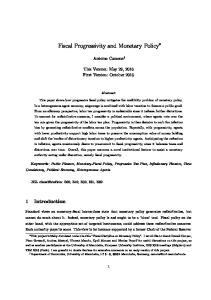
The timing of the model is described as follows and is illustrated in Figure 1. In the beginning of the …rst period, …rms hire workers, rent capital, and produce in each sector. Workers are paid their wage income which is deposited in the bank. Next, banks determine their portfolio allocation. Then, workers learn if they will have to relocate. Movers liquidate their assets. In the beginning of the next period, non-movers will purchase a home with the accumulated savings. Movers transition to their new locations. Movers use their bank returns to consume the consumption good while non-movers’ level of consumption derives from their net income after …nancing housing expenditures. In the following period, non-movers liquidate their homes and use the proceeds to …nance consumption.
Figure 1: Timing of Events 5
2.1 2.1.1
Trade Factor Markets
At the beginning of every period production takes place and input factors are paid. Factor markets are perfectly competitive so factors are paid their marginal products. Consumer good producers rent physical capital from banks and use the labor provided by young agents to produce. Wages are given by:
wt = A(1 The rental rate for physical capital is t
t
)kt
(3)
1
(4)
:
= A kt
Home builders use a single input, residential capital, which it rents from the bank at the rental rate rt : rt = Ph;t B 2.1.2
(5)
Housing Demand
As previously stated, non-movers purchase homes based upon their accumulated savings in their middle-age. In contrast, individuals who experience relocation shocks consume all of their savings during middle age, leaving no resources to consume while old. A non-mover’s accumulated wealth in their middle-age is equal to the return on their savings rtn wt in which rtn denotes the return a non-mover will earn from deposits in the amount wt : Housing demand by non-movers solves the following problem: ) ln(cnt+1 ) +
M ax ln(ht+1 ) + (1 ht+1
ln(cnt+2 )
(6)
subject to: cnt+1 = rtn wt
cnt+2 = (1
Ph;t+1 ht+1
(7)
)Ph;t+1 ht+1
(8)
As housing is a form of wealth accumulation, it also represents a consumptionsavings decision in middle-age. At this time, homeowners reap the utility gains from purchasing a residence. However, it leaves less income available for personal consumption expenditures. In old-age, non-movers use the proceeds from selling their home to …nance consumption. 6
The solution to the individual’s lifetime utility maximization problem generates the following demand for housing:
ht+1 =
( + ) (1 + )
rtn wt Ph;t+1
(9)
As observed in (9), an individual’s demand for housing depends on a number of factors. Of course, the amount of savings a¤ects their home a¤ordability. If individuals value homeownership more (as exhibited by higher values of ), their demand for housing will also be greater. That is, represents the consumption value of homeownership. Moreover, housing is the principal form of savings among the middle-aged. At higher rates of time preference over old-age utility, the ability to save through housing is also an important driver of housing demand. Finally, an individual’s housing demand function is decreasing in the price of the housing stock. In turn, the consumption of a middle-aged person will be:
cnt+1 =
(1 ) n r wt (1 + ) t
(10)
In particular, consumption of middle-aged individuals will be lower if they derive more utility from homeownership and housing expenditures will be relatively high. By comparison, consumption of old-age individuals will be …nanced by their housing wealth:
cnt+2 =
(1
)( + ) (1 + )
rtn wt
(11)
As housing wealth depends on their accumulated savings from their youth, the consumption of old individuals will depend on the interest income earned as well as the utility from owning a home. 2.1.3
The banks’problem
Based upon the anticipated demand for housing of a non-mover, a bank chooses a portfolio assets to acquire on behalf of the middle-aged prior to the realization of the liquidity preference shock. Workers who are relocated must liquidate their deposit balances into money. This liquidity preference shock provides a role for …nancial intermediation by banks. Banks insure individuals against liquidity shocks by pooling their idiosyncratic risks and choosing a portfolio of assets on their behalf. After receiving wage deposits from every worker, the bank allocates deposits between three assets: …at currency (mt ), physical capital (it ), and residential capital (iht ). The
7
allocation of assets is limited by a bank’s deposit base. Hence, the bank’s balance sheet is expressed as: mt + it + iht
wt
(12)
Banks promise returns to both movers and non-movers. The returns to movers and non-movers are denoted as rtm and rtn , respectively. Given that movers must acquire money before they relocate, the return to movers will depend on the amount of money that the bank acquires and the in‡ation rate:
rtm wt
mt
Pt Pt+1
(13)
Comparatively, the return paid to non-movers depends upon the return on the bank’s investment in physical capital and residential capital. The return to physical capital is ; and the return to residential capital is denoted as r: This creates an additional constraint for the bank: )rtn wt
(1
it + iht r
(14)
Since banks are perfectly competitive, the objective of each bank is to maximize the expected lifetime utility among its depositors. However, choosing a portfolio to obtain this objective requires understanding how much non-movers will want to consume in old-age along with their demand for housing. Based upon the anticipated demand for housing, the bank chooses mt , it , and iht to solve:
M ax
ln(rtm wt ) + (1
+ (1
)
mt ;it ;ih t
ln
(1
)
ln
( + ) rtn wt (1 + ) Ph;t+1
+ (1
)( + ) n rt wt (1 + ) s.t. rtm =
rtn =
) ln
(1 ) n r wt (1 + ) t (15)
mt wt
it + (wt (1
Pt Pt+1 mt it )r )wt
wt = mt + it + iht
8
(16)
(17)
(18)
In order for the bank to invest in both sectors of the economy, a no-arbitrage condition between capital in both sectors must be satis…ed:
t
=r
(19)
Money demand is given by: mt =
wt ) +1
(1
(20)
In comparison to the standard two-period random relocation model using logpreferences, the probability of not being relocated factors into the banks’ demand for money. Each bank’s problem involves providing income to di¤erent groups of individuals after the realization of liquidity shocks. For example, non-movers value income which they use in their choice of housing. Their anticipated housing wealth in old-age …nances their old-age consumption. Consequently, the rate of time preference towards old-age utility is a component of money demand by each bank.
2.2
General Equilibrium
We now de…ne the equilibrium for our baseline economy. One of the goals of the model is to determine the amount of housing supply and the relative price of housing. The amount of residential capital in each period depends on previous investment in the residential sector of the economy: h iht = kt+1
(21)
A similar relationship occurs in the non-residential sector: it = kt+1
2.2.1
(22)
Residential Investment
Using the bank’s balance sheet in conjunction with the (19), (3), (21), and (22), we obtain the derived investment demand for residential capital by a bank. The derived investment demand depends on prices and productivity in the residential sector because each intermediary factors anticipated housing demand among nonmovers in choosing the portfolio of assets to acquire on behalf of its depositors:
h Kt+1
= A(1
) (1
)
A
1+ 1 + (1
1
Ph;t+1 B 9
A )
Ph;t+1 B
1 1
(23)
Notably, residential investment is lower at higher prices of housing. At higher prices, individuals who have savings to acquire homes will have lower housing demand. The intermediary factors anticipated demand conditions in choosing the level of residential investment.
2.2.2
Housing Demand and Consumption
Based upon the portfolio choice of the bank, the rate of return to non-movers can be expressed in terms of the price of housing. After substitution into (9), the demand for housing by a middle-aged non-mover is:
ht+1 =
BA(1
)( + )(1 1 + (1 )
)
A
1
Ph;t+1 B
(24)
First, housing demand will depend on net income available after money balances. Higher …nancial returns would then improve the demand for housing. We turn the e¤ects of productivity in the housing sector, B. While it would be natural to assume that productivity is a supply-side factor and only a¤ects housing demand through the price of housing (Ph;t+1 ), housing productivity a¤ects housing demand in our framework through factor markets and …nancial returns. Notably, the higher the return to residential capital in the housing sector (higher values of Ph;t+1 B), the less capital will be allocated to non-residential sector. As a result of lower amounts of investment in the non-residential sector, wages will be lower since labor and non-residential capital are complements in the production of nonresidential goods. However, there is a competing factor due to the higher …nancial returns on savings for non-movers which promotes the demand for housing in (24). Higher levels of total factor productivity (productivity in the non-residential sector) have two e¤ects on an individual’s housing demand. First, productivity in the nonresidential sector raises wages because it attracts more investment. Second, it leads to higher …nancial returns. In addition, there will be more demand for homes (above their role in wealth accumulation) if individuals derive a higher level of utility from homeownership. Higher housing prices are associated with less demand for housing. Armed with …nancial returns and housing demand, we may now determine the levels of consumption among all individuals as a function of housing prices:
cm t+1 =
cnt+1 =
A Ph;t+1 B
1
(1
A(1 1 + (1
)
A )
(25)
Ph;t+1 B
A (1 )(1 + ) ) (1 ) [1 + ( + )]
10
1
BA(1
)( + )(1 ) 1 + (1 ) (26)
Ph;t+1
cnt+2 = (1
2.2.3
)Ph;t+1
BA(1
)( + )(1 1 + (1 )
)
A Ph;t+1 B
1
(27)
Equilibrium in the Housing Market
The total demand for housing comes from aggregating the housing demand across all of the non-movers: Dth = (1
)ht
(28)
We next seek to determine the equilibrium relative price of housing. In each period, new housing supply depends upon residential investment: H = BK h : On the other side of the housing market, demand for new housing depends on the amount that depreciates over time: Dh : The equilibrium price of housing is achieved when total supply and total demand for new housing is the same: Ph;t =
[1 + (1 )] B [1 + ( + )] (1
)
(29)
At higher levels of productivity in the residential sector, the equilibrium price of housing is lower due to the increase in housing supply. Steady-state housing prices also depend on conditions in the non-residential sector. Notably, the capital-share of production in the non-residential sector is associated with higher prices in the housing market. If production in the non-residential sector is more capital-intensive, the capital intensity pulls resources away from the housing market and causes prices to be higher. Prices are also higher if individuals place a higher valuation on utility in old-age which contributes to an increase in housing demand. 2.2.4
Steady-State Equilibrium Macroeconomic Activity
We choose to study macroeconomic activity in the steady-state. As we have shown, steady-state macroeconomic activity is highly dependent on conditions on the housing sector. Therefore, we are able to determine steady-state outcomes across all sectors in the economy with the solution for equilibrium housing prices (Ph ) in (29). After imposing steady-state on the system of equilibrium conditions, we proceed by studying the steady-state levels of investment in each sector which are synonymous with the residential and non-residential capital stocks: + ) Proposition 1. Let < ((1+ ) . Under this condition, a (non-degenerate) steadystate equilibrium exists. In the steady-state, the equilibrium levels of residential and non-residential capital are:
11
A [1 +
K =
K
h
=
A(1
( + )] (1 1 + (1 )
)(1 ) (1 + ) 1 + (1 )
1 1
)(1
1+
)
1 1
(30)
( + ) 1+
1
K
(31)
As previously emphasized, it is important to disaggregate the components of the overall capital stock as the production function varies across sectors. Such di¤erences contribute to substantially di¤erent levels of activity in the steady-state as witnessed by (30) and (31). Moreover, it is also clear that each sector competes for resources – the residential capital stock is the total amount of investment in each period net of investment in the non-residential sector. In addition, fundamentals in each sector have di¤erent e¤ects on investment in the steady-state. Notably, higher levels of productivity in the non-residential sector stimulate investment in both sectors but productivity in the residential sector does not a¤ect investment in either sector. We seek to study how …nancial returns and consumption are determined in the steady-state. For tractability, we look at a special case of capital intensity in the non-residential sector where = 1=2: + ) Lemma 1. Suppose that = 1=2. In addition, let < ((1+ ) : Under these conditions, the steady-state levels of residential and non-residential capital are:
K =
A2 4
Kh =
[1 +
( + )] (1 [1 + (1 )]
( + ) [(1 + ) ( + )]
)
K
2
(32)
(33)
In this case, the connections between both sectors of the economy are quite apparent – the residential capital stock is directly proportional to the non-residential stock of capital. Total factor productivity (A) clearly drives investment in both sectors higher. In addition, there is more investment in both sectors of the economy if liquidity risk is not as severe ( lower). It is also clear that housing fundamentals have asymmetric e¤ects across sectors. Durability of housing leads to less residential investment and more non-residential investment. By comparison, higher valuations for housing services drive residential investment up and lower non-residential investment. 12
We continue by studying steady-state returns in the banking sector and consumption across segments of the population. Returns to Deposits: rm =
rn =
(1
1 1 + (1
) (1
(1 + ) ) [1 +
(34)
)
( + )]
(35)
Returns paid to movers are primarily independent of the return to capital in either sector of the economy. This property re‡ects the logarithmic form of preferences in which the substitution and income e¤ects of higher returns to capital o¤set eachother. In contrast, returns paid to non-movers in the banking sector depend on conditions in both capital sectors. For example, returns are higher if the non-residential sector is more capital-intensive. Moreover, returns to non-movers in the banking sector are higher if fundamentals in the housing sector favor higher housing prices (due to higher rates of depreciation of housing, a greater consumption value of housing, and a greater desire to invest in housing as a form of wealth accumulation). Higher housing prices raise returns to investment in the residential sector of the economy and support the ability of banks to pay higher rates of return to deposits. Steady-State Consumption:
cm =
A2 [1 + ( + )] 4 [1 + (1 )]
(1 ) 1 + (1 )
cn1 =
A2 [(1 + ) ( + )(1 4 [1 + (1 )]
cn2 =
A2 (1 )(1 )( + ) 4 [1 + (1 )]
)]
(36)
(37)
(38)
As a result of the large amount of housing price appreciation before the housing bust, there has been much attention to studying the marginal propensity to consume out of housing wealth. Based upon aggregate data from U.S. states, Case, Quigley, and Shiller (2005) …nd a marginal propensity to consume equal to around 4 cents. Campbell and Cocco (2004) look at micro-level data for households in the UK and …nd that higher housing prices lead to increased consumption among homeowners, but 13
not renters. In contrast, Carroll (2004) …nds that the long-run marginal propensity to consume out of housing wealth to be around 9 cents per dollar. Time-series approaches used to estimate the marginal propensity to consume are constructed in the following way. First, estimate a process for changes in housing wealth. Second, look at a series of changes in consumption. The marginal propensity to consume looks at the slope of the latter process over the former. Interestingly, our framework can be used to draw insights into this phenomenon. In particular, we derive the MPC out of housing wealth when changes in housing wealth are driven by higher levels of productivity. The impact of productivity in the non-residential sector on housing prices is: @(Ph h ) A ( + ) (1 = @A 2 [1 + (1
) )]
(39)
Notably, productivity has a larger impact on housing wealth if individuals derive higher levels of utility from homeownership and they value owning as a form of wealth accumulation because they have a higher rate of time preference. We next turn to studying how productivity a¤ects the consumption of non-movers who are also homeowners: A [(1 + ) ( + )(1 @cn1 = @A 2 [1 + (1 )]
)]
@cn2 A(1 )(1 )( + ) = @A 2 [1 + (1 )]
(40)
(41)
While the e¤ect of productivity of a non-mover in middle-age is decreasing in the value of homeownership, the e¤ect is increasing for the old who …nance their consumption out of housing wealth. Aggregating across both periods is equivalent to looking at the aggregate consumption across both groups of homeowners in the steady-state. As a result, the MPC out of housing wealth is:
MPC =
1+
( + ) (1 ( + ) (1 )
)
(42)
Interestingly, the MPC is exclusively dependent on fundamentals in the housing sector. Of course, the durability of housing is a signi…cant factor. If housing is more durable, housing is a more productive form of wealth accumulation and individuals can spend more as housing wealth increases. It is decreasing in the utility from homeownership –as productivity drives up housing wealth, it is also associated with 14
greater housing expenditures which detracts from the desire of individuals to spend on consumption. The rate of time preference is also a key component of the MPC. In this environment money is super-neutral. However, available evidence indicates that in‡ation does have important e¤ects on housing market activity. We turn to the relationship between in‡ation and housing market activity in the following section.
3
Non-Superneutral E¤ects of Monetary Policy in the Housing Market
In the preceding section, all revenues from seigniorage were consumed by the government. Since the revenues from the in‡ation tax were not redistributed back to the economy, monetary policy was superneutral and did not have any e¤ect on real economic activity. By stripping out real e¤ects from monetary policy, the benchmark framework elucidates how the fundamentals of the housing market a¤ect overall macroeconomic activity. However, the superneutrality of money is clearly at odds with empirical evidence demonstrating that in‡ation has a signi…cant impact on economic activity through the housing sector. For example, both Summers (1981) and Piazessi and Schneider (2012) …nd that housing investment becomes more attractive relative to corporate capital in in‡ationary episodes. Moreover, Ahmed and Rogers (2000) …nd evidence of a longrun Tobin e¤ect for the United States. Thus, the available evidence points to two important observations to address. First, it is important that a model of investment activity produces a positive relationship between in‡ation and investment. Second, monetary policy produces asymmetric e¤ects on investment –residential investment should show a stronger response to in‡ation than non-residential investment. In the following two sections, we seek to address the non-superneutral e¤ects of monetary policy in the housing market and the consequences for macroeconomic performance. Rather than promoting government consumption, in this section, all seigniorage revenues are redistributed to the economy in the form of lump-sum transfers to the young.3 In the next section, seigniorage revenues promote in‡ation-…nanced public credit obligations as in Schreft and Smith (1997, 1998). Due to the revenues from money creation, the government’s budget constraint is:
t
=
1+
mt
(43)
Seigniorage revenues provide the government with income which it redistributes to young individuals in the lump-sum amount, t : Consequently, young individuals have two sources of income. Income from the labor market equal to wt and income from transfers, t : Due to the increase in income, a representative non-mover’s housing demand is: 3 The redistribution of seigniorage to the young is pretty standard in monetary models with liquidity risk. See, for example, Bhattacharya and Singh (2010).
15
( + ) (1 + )
ht+1 =
rtn (wt + Ph
t)
(44)
Consumption across time-periods directly follows the analysis in the benchmark model:
cnt+1 =
(1
cnt+2 =
(1 ) n r (wt + (1 + ) t )( + ) (1 + )
t)
rtn (wt +
(45)
t)
(46)
Obviously, housing demand and consumption are all a¤ected by the transfers from the government. The portfolio choices of the bank are virtually the same as the benchmark model. Again, a no-arbitrage condition implies that the returns to capital in either sector of the economy are the same:
Ph;t B = A Kt
1
(47)
Money balances and the bank balance sheet are a¤ected by the size of the transfers: mt =
(wt +
3.1
(wt + t ) (1 ) +1
t)
(48)
= mt + it + iht
(49)
Steady-State General Equilibrium
As previously stated, workers are paid their marginal product of labor in equilibrium. Combining (47), (49), (43), (48), and (3) we attain a steady-state relationship between residential capital and housing prices that determines the level of residential investment:
h
K = A(1
)
A Ph B
(1
1
(1
16
) (1 + ) ) + 1 1+
!
A Ph B
1 1
(50)
For a given price of housing, higher in‡ation raises seigniorage. With the additional level of deposit income received by the bank, residential investment is also higher. As in the benchmark model, the portfolio choice of the bank provides information about the rate of return to non-movers so that an individual’s housing demand can be expressed as a function of the price of housing: A(1 )B( + ) (1 ) + 1 1+
h=
!
A Ph B
1
(51)
In turn, consumption across the di¤erent segments of the population is:
(1
A(1 ) ) +1
A(1 (1
)Ph B(1 ) ) + 1 1+
cm =
cn1 =
cn2
=
(1
)( + )A(1 (1 ) +1
1+
!
A Ph B
1
!
A Ph B
1
)Ph B 1+
!
(52)
A Ph B
(53)
1
(54)
For a given price of housing, a higher money growth rate stimulates consumption across all segments of the population.
3.2
Equilibrium in the Housing Market
The amount of residential investment a¤ects the total supply of new housing while total demand is equal to Dh : In steady-state equilibrium, prices clear the housing market:
Lemma 2. Let price of housing is:
Ph =
<
( + ) (1+ ) :
B (1
Under this condition, the steady-state equilibrium
)
(1 ) + 1 1+ [(1 + ) ( + ) ] (1
17
)
(55)
A higher money growth rate lowers the price of housing. Further, this impact is stronger if liquidity risk in the economy is higher. Presumably, the lower price of housing in response to higher in‡ation re‡ects an increase in housing supply. In order to sort this out, we turn to the following:
Proposition 2. Let < capital across sectors are:
=
( + ) (1 + )
Under this condition, the steady-state stocks of
A [(1 + ) ( + ) ] (1 (1 ) + 1 1+
K =
Kh
( + ) (1+ ) :
BPh
( + ) A(1 (1 + )
[A (K ) )
)
!
1 1
(56)
BPh K ] +
(1 (1
) (1 + ) ) +1
(57) (1 (1
) (1 + ) ) + 1 1+
!
(K )
Proposition 2 demonstrates how monetary intervention in the economy dramatically changes how housing market activity depends on macroeconomic conditions. In the absence of transfers from seigniorage, (31) is simply the residual amount of capital after non-residential investment. However, (57) is clearly non-linear in the non-residential stock and housing prices. In this manner, our framework demonstrates that policy intervention by monetary authorities is likely to make the interplay between the housing market and macroeconomic activity much less transparent. Nevertheless, analytical solutions for all variables are obtainable in the special case in which the non-residential sector is equally capital and labor-intensive:
Lemma 3. Let = 1=2: Assuming Proposition 1 holds, a (non-degenerate) steady-state equilibrium exists. In the steady-state, the equilibrium stocks of residential and non-residential capital are:
K =
A2 4
(1
) ((1 + ) 1 + (1 )
18
( + ) ) 1+
!!2
(58)
Kh =
( + ) (1 + ) ( + )
K
(59)
As previously mentioned, Ahmed and Rogers (2000) …nd evidence of a long-run Tobin e¤ect for the United States. It is clear from (58) and (59) that higher rates of in‡ation stimulate investment activity in both sectors of the economy. However, where does monetary policy have the biggest impact? We turn to this issue in the following corollary to Lemma 3:
3.2.1
The E¤ects of Monetary Policy
The principal objective of this section is to focus on the e¤ects of monetary policy. Based upon Lemma 3, it is easy to see that the e¤ects of monetary policy in the housing sector are proportional to the e¤ects of policy in the non-residential sector:
@K h = @
( + ) (1 + ) ( + )
@K @
Corollary 1. Assume that the conditions in Lemma 3 hold. Further, let h > @K > 0: If these conditions hold, @K @ @
(60)
>
(1+ ) 2( + ) :
According to the corollary, monetary policy will have asymmetric e¤ects on the residential and physical capital stocks. In particular, as observed in the empirical evidence, in‡ation has a stronger e¤ect on the residential capital stock than the physical capital stock. Thus, monetary policy plays a bigger role in investment in the housing sector than the non-residential sector. It is often argued that the reason for such behavior is due to the interest-rate sensitivity of the housing sector. Alternatively, the mortgage-interest deductibility through taxes if often cited. However, our framework demonstrates that the durability of the housing stock is a signi…cant factor. Simply put, housing is a durable asset. As a result, in‡ation promotes the asset with the highest present discounted stream of income. Arnott (1980) also stresses that the durability of housing should be an important consideration when evaluating the e¤ects of public policy. 19
While Corollary 1 demonstrates that the e¤ects of monetary policy are stronger in the housing sector than the non-residential sector, the following focuses on conditions in the non-residential sector: Corollary 2. Assume that the conditions in Lemma 3 hold. The physical capital locus, (58), behaves such that:
@K @2K @2K > 0; > 0; <0 @ @ @A @ @
While Corollary 1 demonstrates that in‡ation promotes capital accumulation, Corollary 2 demonstrates that the e¤ects of policy are stronger if productivity in the economy is higher. However, the e¤ects of in‡ation are weaker if preferences for housing are higher. Yet, our principal motivation is to study the impact of policy on housing market activity in general equilibrium:
Corollary 3. Assume that the conditions in Lemma 3 hold. The equation denoting the residential capital stock, (59), behaves as follows:
@K h @2K h @2K h @2K h > 0; > 0; > 0; > 0 if @ @ @A @ @ @ @
<
(1 + )(1
)
2
2
In‡ation raises the residential capital stock by way of increasing the income of young workers. The revenues from the in‡ation tax are also higher if wages are higher which explains the complementarity between monetary policy and productivity. Thus, the model demonstrates that monetary policy would be less e¤ective in promoting housing market activity in periods of low productivity than high productivity. For example, attempts to promote economic activity during the productivity slowdown of the 1970s were largely unsuccessful. However, residential investment was consistently higher during the high levels of productivity encountered in the “New Economy”from 1993 - 2003. The latter period has also been characterized as a period 20
in which homeownership rates climbed. For example, in 1970, the U.S. Census reports that the homeownership rate was 62.9%. It climbed to 64.2% in 1990 and 66.2% in 2000. The apparent increase in preferences for homeownership also contributed to the strong impact of policy on housing market activity. We next turn to the impact on policy on consumption. Steady-State Consumption:
cm =
A2 [(1 + ) ( + ) ] (1 ) h i2 4 (1 ) + 1 1+
cn1 =
cn2 =
A2 (1
h
4 (1
h
)
) +1
A2 (1
4 (1
1+
)( + ) ) +1
1+
(61)
i
(62)
i
(63)
As in the previous section, we are particularly interested in …nding the determinants of the MPC from housing wealth. In contrast to the benchmark model, monetary policy has real e¤ects on the housing market:
@(Ph h) = @
h
4 (1 + )2 (1
A2 ( + ) ) +1
1+
i2
(64)
That is, although monetary policy leads to an increase in residential investment, the increase in supply lowers the total value of the housing stock. We next turn to the e¤ects of policy on consumption across the consumption path: 21
@cn1 = @
@cn2 = @
h 4 (1 + )2 (1
A2 (1
)
) +1
A2 (1 h 4 (1 + )2 (1
1+
)( + ) ) +1
1+
i2
(65)
i2
(66)
By inducing individuals to allocate more income towards housing, consumption declines. Hence, the marginal propensity to consume out of housing wealth di¤ers in comparison to the benchmark model:
MPC =
1+
( + ) ( + )
(67)
Moreover, the MPC di¤ ers when housing wealth is driven by real factors such as productivity in comparison to nominal factors such as monetary policy. This is an important argument that policymakers need to consider when trying to understand how consumption patterns respond to changes in housing market activity over time.
4
The Economy with Government Bonds
In recent years, the line between …scal policy and monetary policy has become blurred as many have argued that the high amount of money growth that has occurred across countries simply represents a redistribution to …scal authorities. In order to consider this possibility, we extend the model to account for in‡ation-…nanced government bonds as in Schreft and Smith (1997, 1998). In this manner, there is another asset for banks to add to their portfolios. As in the previous setting with transfers from seigniorage, monetary policy in this setting is not super-neutral. With the introduction of government debt, banks now allocate deposits between money, physical capital, residential capital, and bonds. The real per capita bond Bt Pt supply is bt Pt ; and the real return on bonds is Rt = It Pt+1 ; where It is the nominal interest rate. We assume there are no government transfers or taxes. Therefore, the government budget constraint requires:
22
Rt
1 bt 1
=
(Mt
Mt Pt
1)
+ bt
(68)
Government revenue must be su¢ cient to cover interest payments on previously issued bonds. Revenues come from newly issued bonds along with seigniorage. Given the bank now has four asset choices, the bank’s balance sheet is:
wt = mt + it + iht + bt
(69)
The return paid to movers comes from the bank’s money balances:
rtm wt = mt
Pt Pt+1
(70)
In comparison, the return to non-movers is paid from the bank’s return on physical capital investment, residential investment, and bond holdings.
(1
)rtn wt = it + iht r + Rt bt
(71)
The bank’s objective is to maximize the expected utility of its depositors. In order for banks to invest in both types of capital and govnerment bonds, the following two no-arbitrage conditions must hold:
Ph;t B = A Kt It
1
= Ph;t B
(72)
(73)
As in the benchmark model, money demand is:
mt =
(1
wt )(1
23
)+
(74)
4.1
Steady-State General Equilibrium
By virtue of the no-arbitrage conditions which apply, the total demand for housing is the return on income after money balances:
Dh =
( + ) 1 (w (1 + ) Ph
m)r
(75)
In the steady-state, bond demand is:
b=
1 I
m
(76)
Similar to the previous model, in equilibrium the supply of housing must equal the total demand for housing: BK h = Dh
(77)
A steady-state equilibrium reduces to two conditions on the residential capital stock and the nominal return to bonds which must hold. The …rst condition derives from the government’s budget constraint (GBC ):
Proposition 3. (Government Budget Constraint) Suppose that (1 )(1 ) > I : Also, assume that I < : Under these conditions, the residential capital stock is positive and described by:
h
K = A(1
)
A I
1
0 @
(1
)(1 (1
)(1
24
)
( (I
)+
1) )
1 A
A I
1 1
(78)
In addition,
@K h @I j78
and
@K h j78 > @
0:
In equilibrium we are interested in analyzing the economy when I > 1. This insures that the return on money is dominated by the return from other assets. However, as I < , this implies that the revenues earned from money creation exceed the interest paid on government bonds. Hence, b < 0. That is, the residential capital stock only exists as long as the government is a net lender to the …nancial system. Typically, in models such as Schreft and Smith (1997, 1998), the government budget constraint has two potential positions. If I > , the government is a net borrower since the interest to pay for its debt exceeds seigniorage revenues. The other position is similar to the result in Proposition 3. In the presence of government bonds, residential investment competes with bonds and the non-residential sector for resources. As suggested by the Proposition, if the government were a net borrower, it would require the housing stock to be negative. In contrast, a higher money growth rate provides the …scal authority with more resources to support housing market activity. The second condition that must hold is that the housing market must be in equilibrium:
Kh
Proposition 4. (Housing Market Equilibrium) The relationship between I and in which (77) is satis…ed is described by:
h
K =
In addition,
( + ) (1 + )
@K h @I j79
"
A(1
< 0 and
)
A I
@K h j79 > @
(1
1
(1
)(1 ) )(1 )+
#
(79)
0:
Steady-state locus, (79), represents equilibrium in the housing market. More speci…cally, (79) demonstrates how the nominal interest rate must relate to residential capital to ensure the demand for housing is equivalent to the supply of housing. As demonstrated by the Proposition, there is a negative relationship between the 25
nominal interest rate and the residential capital stock. At higher nominal interest rates, the return to government bonds is higher. As a result, banks allocate more resources to bonds which results in lower residential investment. However, higher money growth reduces the real return to bonds and induces a substitution towards residential capital. Based upon the above analysis, we arrive to the following Proposition:
Proposition 5. Suppose that
( + ) (1+ )
) + [(1 (1)(1 ) )+ ] < (1 )(1 )+ steady-state exists in which I < :
A > (1
)+ 1
as I ! 1 and
( + ) (1+ )
(1
as I ! 1: If these conditions hold, a unique
Figure 2 depicts the Government Budget Constraint and Housing Market Equilibrium loci in which an equilibrium exists.
Figure 2: Steady-State Equilibrium
In the following, we discuss the e¤ects of monetary policy in the presence of government bonds.
26
4.1.1
The E¤ects of Monetary Policy
We now focus on the e¤ect of monetary policy on the residential capital stock. As opposed to Schreft and Smith (1997, 1998), only one steady-state exists so the e¤ects of monetary policy on capital accumulation can be pinned down. To begin, as previously mentioned in Proposition 3, a higher money growth rate shifts the locus (78) to the right. We refer to this shift as the redistribution e¤ ect from monetary policy as it is associated with the bank’s allocation from nominal to illiquid assets and thereby induces redistribution from movers to non-movers when residential investment increases. From Proposition 4, a higher rate of in‡ation also shifts the locus associated with (79) to the right. This re‡ects the substitution e¤ ect from monetary policy as in‡ation reduces the real return to government bonds. Consequently, banks allocate more funds towards residential investment. The total increase in residential investment due to both mechanisms is shown in Figure 3 below:
Figure 3: Increase in the Rate of Money Growth
5
Optimal Monetary Policy
The previous two sections provide mechanisms in which in‡ation promotes housing market activity. In fact, each model shows that the impact of in‡ation is permanent – that is, higher in‡ation rates promote investment and housing market activity from any in‡ation rate. However, the U.S. in‡ationary experience in the 70s shows 27
that there are limits to the potential bene…ts from higher in‡ation. For example, Bernanke (2004) contends that high in‡ation contributed to output volatility and high unemployment during the 1970s. Romer and Romer (2002) make the same arguments. We incorporate the relationship between volatility and risk observed in the data by assuming that the incidence of liquidity risk is a function of monetary policy, ( ): In particular, we posit that the marginal increase in risk is higher at high in‡ation rates. Therefore, we consider the case where ( ) = (1 + d )2 : Similar ideas have been proposed in the literature. For example, Ghossoub and Reed (2010) study a model in which the incidence of liquidity risk is a function of the capital stock. They argue that such a mechanism captures the increased exposure to risk in poor countries relative to the stability of advanced economies. Our objective is to show that introducing the relationship between policy and volatility allows us to formalize the trade-o¤s inherent in designing policy to stimulate housing market activity. In particular, we demonstrate that these trade-o¤s are important for thinking about how optimal monetary policy depends on conditions in the housing market. To show the impact of policy, we return to a setting in which seigniorage revenues are transferred to the young. We de…ne welfare as the expected lifetime utility of an individual young agent:
n m U (cm t+1 ; ct+1 ; ht+1 ; ct+2 ) = ( ) ln(ct+1 )+(1
( ))
ln(ht+1 ) + (1
) ln(cnt+1 ) +
ln(cnt+2 )
We characterize “optimal” monetary policy by the choice of that would maximize welfare. In terms of our numerical analysis, we start by identifying the optimal rate of in‡ation given our choice of parameters. We consider the following parameter set: A = 7:4; B = 4:8, = :8, = :33; = :5; d = 9:7; = :35, and = :3: Also, in order to maintain consistency with the majority of the previous analytical results, we assume that the non-residential sector is equally capital and labor-intensive. The primary point of our parameter set is that the welfare-maximizing rate of in‡ation is = 0:03: This is demonstrated in Table 1 below and is consistent with the average in‡ation rates during the Volcker-Greenspan era of monetary policy, the “Great Moderation.”
28
Kh K m w Ph h Ph h welf are
0:015 1.74612 3.87525 1.68726 7.28369 .391571 25.3981 .0249349 6.45678 3.00459
Table 1 Optimal monetary policy 0:02 0:025 0:03 0:035 1.74883 1.75119 1.75319 1.75484 3.87613 3.87472 3.87104 3.86507 1.69275 1.69871 1.70517 1.7121 7.28452 7.2832 7.27973 7.27412 .391527 .391598 .391784 .392086 25.4376 25.4719 25.501 25.525 .0331911 .041432 .049665 .0578972 6.46015 6.46241 6.46355 6.46358 3.00553 3.00607 3.0062 3.00593
0:04 1.75614 3.85684 1.71953 7.26637 .392504 25.5438 .0661356 6.46249 3.00526
0:045 1.75708 3.84635 1.72744 7.25648 .39304 25.5576 .0743872 6.46028 3.00419
In comparison to the model with transfers, higher rates of in‡ation promote residential investment but not investment in the non-residential sector. However, higher in‡ation rates are associated with higher housing prices which is consistent with available evidence. We turn to examining the role that housing market fundamentals play in determining optimal monetary policy. We begin with a setting in which productivity in the housing sector is lower (B = 2:4). This may be due to increased land regulations over time. The results are listed in Table 2:
Kh K m w Ph h Ph h welf are
0:024 1.75075 3.87519 1.69748 7.283149 .783149 12.7327 .0397847 6.46205 2.87123
Table 2 Optimal monetary policy (B = 2:4) 0:027 0:03 0:033 0:036 1.75204 1.75319 1.75423 1.75513 3.87352 3.87104 3.86733 3.86361 1.70124 1.70517 1.70927 1.71355 7.28207 7.27973 7.27662 7.27274 .783317 .783568 .783903 .784321 12.7421 12.7505 12.758 12.7646 .0447258 .049665 .054604 .0595442 6.463 6.46355 6.4637 6.46345 2.87152 2.87167 2.87169 2.87158
0:039 1.75591 3.85867 1.718 7.26809 .784823 12.7702 .0644871 6.46279 2.87133
0:042 1.75656 3.85292 1.72263 7.26267 .785409 12.775 .0694343 6.46172 2.87096
In response to the lower productivity, supply in the housing market will be lower. Consequently, access to housing would be lower. In order to promote housing market activity, the optimal rate of money growth is raised to = 0:033: As a result, residential investment will increase and promote housing supply in the face of low productivity. In this manner, optimal monetary intervention should be more aggressive in economies with adverse housing supply conditions. 29
We conclude by looking at a setting in which there is an increase in housing demand. This is due to the higher consumption-value of home ownership:
Kh K m w Ph h Ph h welf are
0:01 1.89136 3.26419 1.54456 6.68482 .426651 27.5106 .0152927 7.62535 3.15788
Table 3 Optimal monetary policy ( = :5) 0:015 0:02 0:025 0:03 1.89454 1.89726 1.89953 1.9013 3.26631 3.26627 3.26409 3.25976 1.54903 1.55389 1.55912 1.56475 6.68698 6.68695 6.68471 6.68028 .426513 .426515 .426658 .426941 27.5569 27.5965 27.6295 27.6559 .0228921 .0304683 .0380274 .0455753 7.63071 7.63472 7.6374 7.63875 3.15907 3.15972 3.15985 3.15944
0:035 1.9027 3.25329 1.57077 6.67364 .427365 27.6757 .053178 7.63877 3.15852
0:04 1.90362 3.24468 1.57717 6.66481 .427932 27.689 .0606604 7.63748 3.15706
If individuals value homeownership more, the optimal monetary policy rule seeks to reduce volatility in the economy. This promotes the ability of individuals to save so that they face less exposure to liquidity risk. As a result, the optimal rate of in‡ation falls to = 0:025: That is to say, monetary policy should be more conservative if fundamentals in the economy favor housing demand.
6
Conclusion
In recent years, the impact of monetary policy on housing markets and the macroeconomy has received a large amount of attention. This paper provides a dynamic general equilibrium model with a microfoundation for money to study the transmission of monetary policy to the housing sector and macroeconomic activity. While previous empirical work has shown that in‡ation stimulates housing sector activity, our research develops a rich framework to show that there are important asymmetries resulting from monetary stimulus. As in a large volume of work on housing, we show that the durability of housing as an asset plays a huge role. Moreover, we study how optimal policy intervention depends on conditions in the housing sector. Interestingly, we …nd that optimal money growth is higher if productivity in the residential sector is low. In this manner, we argue that policy should be designed according to supply conditions in the housing sector. By comparison, in‡ation should be lower when conditions favor housing demand. There are a number of issues we intend to address in future work. For example, the model could be extended as in Arnott et al. (1999) to study the impact of monetary 30
policy on investment in both housing quantity and quality. Investment in multifamily structures could also be incorporated. In addition, both Arnott and Braid (1997) and Harding et al. (2007) look at housing maintenance and depreciation over time. One could also use our framework to show how in‡ation plays a role in housing sector activity through endogenous maintenance expenditures. Finally, Mankiw and Weil (1989) point out that population demographics have important consequences for housing prices. Consequently, we intend to study how optimal monetary intervention depends on demographics in future work.
31
References Ahmed, S. and J.H., Rogers, 2000. In‡ation and the Great Ratios: Long Term Evidence From the U.S. Journal of Monetary Economics 45, 3-35. Albouy, D. and G. Ehrlich, 2012. Metropolitan Land Values and Housing Productivity, NBER Working Papers 18110, National Bureau of Economic Research, Inc. Arnott, R.J., 1980. A Simple Urban Growth Model with Durable Housing. Regional Science and Urban Economics 10, 53-76. _____, and _____, 1997. A Filtering Model with Steady-State Housing. Regional Science and Urban Economics 27, 515-546. _____, R. Braid, R. Davidson, and D. Pines, 1999. A General Equilibrium Model of Housing Quality and Quantity. Regional Science and Urban Economics 29, 283-316. Bernanke, B.S., 2004. The Great Moderation. Remarks at the meetings of the Eastern Economic Association, Washington, D.C., federalreserve.gov/boarddocs/speeches/2004/20040220. Bhattacharya, J. and R. Singh, 2010. Optimal Monetary Policy Rules under Persistent Shocks. Journal of Economic Dynamics and Control 34, 1277-1294. Campbell, John Y. and Joao F. Cocco. 2007. How Do House Prices A¤ect Consumption? Evidence from Micro Data. Journal of Monetary Economics 54, 591621. Carroll, C.D., 2004. Housing Wealth and Consumption Expenditure. Paper prepared for Academic Consultants Meeting of Federal Reserve Board, January. Case, K.E., J.M. Quigley, and R.J. Shiller, 2005. Comparing Wealth E¤ects: The Stock Market Versus the Housing Market. Advances in Macroeconomics 5, 1235-1235. Diamond, D. and P. Dybvig, 1983. Bank Runs, Deposit Insurance, and Liquidity. Journal of Political Economy 90, 881-894. Epple, D., B. Gordon and H. Sieg, 2010. A New Approach to Estimating the Production Function for Housing. American Economic Review 100, 905-924. Fama, E. and Schwert, G., 1977. Asset returns and in‡ation. Journal of Financial Economics 5, 115–146. Ghossoub, E. and R.R. Reed, 2010. Liquidity Risk, Economic Development, and the E¤ects of Monetary Policy. European Economic Review 54, 252-268. Ghossoub, E.A. and R.R. Reed, 2013. The Stock Market, Monetary Policy, and Economic Development. Southern Economic Journal 79, 639-658. Glaeser, E., J. Gyourko, and A. Saiz, 2008. Housing Supply and Housing Bubbles. Journal of Urban Economics 64, 198-217. ____, _____, and R. Saks, 2005a. Urban Growth and Housing Supply. Journal of Economic Geography 6, 71-89.
32
____, ____, and _____, 2005b. Why is Manhattan so Expensive? Regulation and the Rise in Housing Prices. Journal of Law and Economics 48, 331-369. Harding, J.P., S. Rosenthal, and C.F. Sirmans, 2007. Depreciation of Housing Capital, Maintenance, and House Price In‡ation: Estimates from a Repeat Sales Model. Journal of Urban Economics 61, 193-217. Kocherlakota, N., 2003. Societal Bene…ts of Illiquid Bonds. Journal of Economic Theory 108, 179-193. Mankiw, G.N. and D.N. Weil, 1989. The Baby Boom, The Baby Bust, and the Housing Market. Regional Science and Urban Economics 19, 235-258. Piazzesi, M., and Schneider, M., 2012. In‡ation and the Price of Real Assets. Working Paper. Romer, C. D. and D.H. Romer, 2002. The Evolution of Economic Understanding and Postwar Stabilization Policy. Proceedings, Federal Reserve Bank of Kansas City, 11-78. Schreft, S.L. and B.D. Smith, 1997. Money, Banking, and Capital Formation. Journal of Economic Theory 73, 157-182. ______ and ______, 1998. The E¤ects of Open Market Operations in a Model of Intermediation and Growth. Review of Economic Studies 65, 519-50. Summers, L. 1981. In‡ation, the Stock Market, and Owner-Occupied Housing. AEA Papers and Proceedings 71, 429-434.
33