School Of Computer Science MSc. in Natural Computation

Mini Project 1

Heuristic Scheduling Based on Policy Learning Vineet Khare

Supervisor: Dr. Thorsten Schnier

January 2002

Abstract Combinatorial Optimisation problems are generally NP-complete problems, which means that solving the problem needs exponential time. Thus heuristic methods are preferred over exact methods, like dynamic programming and branch and bound. Scheduling is one such combinatorial optimisation problem. Another problem with using these exact methods in scheduling is that it is quite difficult to formulate mathematically. For instance, it is very common for the constraints and objectives of the problem to conflict. I am looking at some of the heuristic techniques used in literature for scheduling. Specifically those techniques which learn policies either from their past experience or from simulation. These policies are local and answer the question, "What is the best way to generate a GOOD solution?" The consistent following of the policy at the local level gives a solution that is perhaps not truly optimal, but is nevertheless good (enough). I will also assess the relative strength of these methods considering (1) Their reported performance on benchmark problems (2) Their robustness to unforeseen events.

Keywords Heuristic, scheduling, policy learning, inductive learning, reinforcement learning, expert system, knowledge modification, genetic algorithms, neural networks, genetic programming.

ii

Acknowledgements I would like to take this opportunity to thank all those who painstakingly guided me during the project. I acknowledge the efforts of the following people and thank them for their help and co-operation. Without their help and guidance I would not have been able to complete this project. First of all I would like to thank Dr. Thorsten Schnier for his constant encouragement and for his useful suggestion from time to time. I would like to thank Dr. P. J. Hancox useful suggestions regarding literature searching and report writing. Thanks are also due to Mr. Graham Hesketh, industrial supervisor for the project, for providing relevant references related to the topic and to Prof. Y. Yih, Purdue University, for sending me her papers on the topic. Vineet Khare

iii

Contents Abstract .....................................................................................................................................ii Keywords...................................................................................................................................ii Contents ...................................................................................................................................iv List Of Figures .........................................................................................................................vi List Of Tables .......................................................................................................................... vii 1.

Introduction ..................................................................................................................... 1 1.1 Scheduling................................................................................................................... 1 1.2 Global Vs. Local Techniques ..................................................................................... 1 1.3 Mini-Project Proposal ................................................................................................. 2 1.4 Organization of the Report......................................................................................... 2

2.

Heuristic Rule Learning .................................................................................................. 3 2.1 Heuristic Rules............................................................................................................ 3 2.2 Learning Heuristic Rules............................................................................................ 3

3.

Literature Review ............................................................................................................ 5 3.1 Probabilistic Learning Combinations of Local Job-Shop Scheduling Rules......... 5 3.2 Iterative Dichotomister 3 ............................................................................................ 6 3.3 Trace Driven Knowledge Acquisition (TDKA)........................................................... 7 3.4 Knowledge Based Dynamic Scheduling System ..................................................... 8 3.5 Pattern Directed Scheduling ...................................................................................... 9 3.6 Reinforcement Learning Approach to Job-Shop Scheduling Problems .............. 10 3.7 Integration of Inductive Learning and Neural Networks (IL/NN) for FMS scheduling.......................................................................................................................... 12 3.8 Genetic Reinforcement Learning Approach to Heterogeneous Machine Scheduling ......................................................................................................................... 13 3.9 Learning to Solve Planning Problems Efficiently by Means of Genetic Programming ..................................................................................................................... 13

iv

4.

Critical Review............................................................................................................... 15 4.1 Reported performance on various problems – Merits & Demerits ....................... 15 4.2 Comparison ............................................................................................................... 20

5.

4.2.1

Benchmark Performance................................................................................... 20

4.2.2

Robustness to unforeseen events ...................................................................... 21

4.2.3

Understand-ability of derived policies................................................................. 21

Future Work – Summer Project Proposal.................................................................... 22 5.1 Project proposal........................................................................................................ 22 5.2 Basic Scheduling Scenario from Rolls-Royce........................................................ 22 5.3 Possible solution strategy – using IL/NN approach............................................... 24

6.

Conclusion..................................................................................................................... 26

7.

References ..................................................................................................................... 27

Appendices A Mini-project declaration B Statement of information search strategy

v

List Of Figures

Figure 1 - 6 X 6 X 6 Test Problem (Times in parentheses) ........................................................ 5 Figure 2 - A Simple Decision Tree ............................................................................................. 6 Figure 3 - Model of TDKA .......................................................................................................... 8 Figure 4 - Architecture of knowledge based dynamic scheduling system .................................. 9 Figure 5 - Framework for PDS ................................................................................................. 10 Figure 6 - Development of multi-objective FMS scheduler ....................................................... 12

vi

List Of Tables Table 1: Strategies and rules for selection ................................................................................. 4 Table 2 - Performance measures and dispatching rules .......................................................... 17 Table 3 - Yield of simple production line operated by resulting rules and by three best schedulers. Performance is equal to good*(good /(good+bad)). ..................................... 20 Table 4 - PDS performance...................................................................................................... 21 Table 5 - Scheduling scenario.................................................................................................. 23 Table 6 - Associated Rules [used by Yih et al. (1998)]............................................................. 24

vii

1. Introduction 1.1

Scheduling

Scheduling in general deals with assignment of activities to limited recourses where a set of constraints has to be regarded. These constraints can be e.g. restrictions on the ordering of operations, due dates etc. In most cases one of the objectives is to minimize the overall time taken to complete all the required operations. Examples of this very general problem include scheduling university exams (the 'time-tabling' problem) or the distribution of work amongst machines in a machine-shop (the so-called 'job-shop scheduling’ problem). Minimizing overall production time helps the companies to meet the due dates, satisfy the customers and to respond to flexible market demand. But also other goals e.g. cost reduction are important and often a mix of different goals is found which makes finding a good schedule a difficult task. Scheduling problems are found in a lot of application domains. Besides production there are also other applications like scheduling of airline crews space missions, timetabling and processor scheduling etc. Sauer (1999) broadly classified scheduling as: 1. Predictive Scheduling: Creating a schedule in advance for a period of time. 2. Reactive Scheduling: Here schedules are repaired due to actual events (machine breakdown, new or cancelled order) in the scheduling environment. Schedule has to be adapted to the new situation using appropriate actions to handle each of the events. 3. Interactive Scheduling: It combines both predictive and reactive scheduling with the requirements of a user who wants to keep the decisions in his hands, e.g. introducing new orders, cancel orders, change priorities set operations to specific schedule positions, and there decisions have to be regarded within the scheduling process.

1.2

Global Vs. Local Techniques

Scheduling can be regarded as a combinatorial optimisation problem, i.e., the problem of optimising an evaluation function with respect to a given scheduling problem. Most of the problems requiring an optimal are NP-complete problems, which means that solving the problem needs exponential time. In order to determine an optimal solution, different restrictions have been imposed on the problem domain (e.g., on the number of orders or machines), which makes the application of the results to real world scheduling problems very difficult or even impossible because most of the constraints of the scheduling environment are not regarded. Due to the difficulty of finding optimal solutions, we prefer a "good" and feasible solution regarding all the objectives and preferences of the scheduling environment, which might not be optimal but is good (enough). Very important for this task is the (heuristic) knowledge of the human domain expert who is able to solve distinct scheduling problems and to judge the feasibility of schedules by virtue of his/her gained experience.

1

Human problem-solving also centres more on the application of heuristics or a "policy" which shifts the focus away from the question "what IS the best solution to the problem" and instead focuses on the question "what is the best way to GENERATE a good solution". In this way it is hoped that the consistent following of the policy at the local level will result in an emerging global behaviour. Such local actions may be taken based on information about the global state of affairs, or may be taken based on a more restricted set of facts available to the decision unit. In terms of the job-shop scheduling problem, such a policy might be envisaged as one which answers the question "which batch of components should I process next on this machine?" given knowledge about the current state of affairs.

1.3

Mini-Project Proposal

Aim of mini-project: To find out the methods for the derivation of heuristic rule based policies for scheduling and to assess their relative strengths. Objectives to be achieved: 1. To research the literature and report on methods for the derivation of heuristic rule based policies for scheduling. 2. Assess these methods on benchmark problems. 3. Assess their robustness to unforeseen events. 4. To find out the degree to which the derived policies can be understood by human beings.

1.4

Organization of the Report

The rest of this report is organized as follows: In Section 2, I have discussed heuristic rules and rule learning. Section 3 describes various methods from literature that involve heuristic rule learning. Section 4 presents the critical review of some of these methods – it includes reported performance on various problems and comparisons between the techniques. Finally, Section 5, presents a practical scheduling problem from Rolls-Royce with a possible solution strategy.

2

2.

Heuristic Rule Learning

Before looking into the scheduling techniques that learn heuristic rules, lets first look at what are these rules and why is it important to learn these rules. Machine scheduling in most production systems is done by allocating priorities to jobs waiting at various machines through these dispatching heuristics.

2.1

Heuristic Rules

These are Simple priority rules based on information available related to jobs. In the context of production scheduling, job shop scheduling rules are the ones that can be applied by machine operators and that require only his knowledge of the work that is waiting for his machine to perform. Heuristic scheduling is based on heuristic search techniques such as problem decomposition together with problem specific knowledge adopted from scheduling experts in order to guide the search process. Heuristic rules can guide the search, depending upon the knowledge available about the requirements and constraints, e.g. Information Available Processing Time Due dates Slack Arrival Time

Rule Shortest processing time (SPT) Earliest Due Date (EDD) Minimum Slack (MINISLK) First in first-out (FIFO)

Some of the rules for selection, depending upon the problem decomposition given by Sauer (1999) are given in Table 1.

2.2

Learning Heuristic Rules

In most of the techniques that use heuristic rule learning knowledge about a problem domain is encoded in some structure (rules, logic, frames etc) and manipulated to solve a problem. Domain knowledge of interest to a person is knowledge about the scheduling in his specific production environment. These knowledge-based methods are often known as AI methods. Some of the simpler knowledge based methods are Expert system (ES) methods, which simply duplicate the decisions made by human experts. These are constructed by, first acquiring knowledge from a human expert and then codifying this knowledge in some knowledge representation scheme (rules, frames etc.). But this knowledge acquisition usually involves time-consuming interviews with the human experts. Another problem with ES is that human experts have a limited cognitive competence and as the production environment complexity increases they tend to be less effective as observed by Savell, Perez, Koh (1989). Furthermore ES can only automate the decisions made by human experts- good or bad. An ES can never outperform the human expert.

3

Hence the system in itself should be able to adapt to the changing environment, it should include learning components to correct its misconceptions and improve its performance based on experience.

For the selection of orders • Schedule order with earliest start time first (EST-rule) • Schedule order with earliest due date first (EDD-rule) • Schedule order with shortest processing time first (SPT-rule) • Schedule order by increasing number of alternatives (critical products first) • Schedule order by increasing slack intervals • Schedule order by increasing user priority For the selection of routings • Use stem variant first (ranking of routings necessary) • Select in inverse order (LCFS) • Use critical routing first (use heuristic to find critical routing) • Use simple routing first (use heuristic to find simple routing) • For the selection of operations For the selection of operations • Select by increasing operation number (FCFS) • Select by decreasing operation number (LCFS) • Select critical operation first (e.g., by increasing number of alternative resources) • Select simple operation first (e.g., by decreasing number of alternative resources) For the selection of resources • Use stem first (ranking of resources necessary) • Use simple resource first (use heuristic to find simple resource) • Use critical resource first (use heuristic to find critical resource) For the selection of intervals • Forward from given release date • Backward from due date (JIT). For conflict resolution • Look for alternative time interval within given time window • Look for alternative resource • Look for alternative routing • Change given time window Table 1: Strategies and rules for selection

4

3. Literature Review In this section I will be reviewing the techniques available in literature that involve any kind of policy learning for scheduling. For learning we should first develop a knowledge base and keep on modifying it. The first step in developing a knowledge base is knowledge acquisition. This in itself is a two-step process- Getting the knowledge from knowledge sources and store that knowledge in digital form. Knowledge sources may be human experts, simulation data etc. To extract knowledge from these sources we can use machine-learning techniques that can learn from examples. In general all the techniques follow these four steps: 1. Obtaining knowledge from sources (Human Expert, Simulation data) 2. Store this knowledge in digital form (e.g. decision trees). 3. Making Decision at various points of scheduling. 4. Modification of stored knowledge. Now lets see some of the techniques that use some kind of heuristic learn. The first one that I have found out was given by Fisher and Thompson (1963).

3.1

Probabilistic Learning Combinations of Local Job-Shop Scheduling Rules

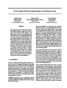
Fisher and Thompson (1963) used combination of two heuristic rules, Shortest Imminent Operation (SIO) (Also known as First On First Off (FOFO)) rule and Longest Remaining Time(LRT), in scheduling. One of the sample problems they used is shown in Figure 1. There are six goods and six machines, and each good must be processed by each machine in the order shown. The times for various operations are indicated in parentheses after the facility number.

Figure 1 - 6 X 6 X 6 Test Problem (Times in parentheses)

5

Using the combination of SIO and LRT rules they tried to minimize the completion time. Which rule to choose, at a particular decision point, was selected either by an unbiased random process or by using a learning process. • Generating good results by an unbiased random process: A rule is selected at random among the set of local decision rules. The random process performs invariably better than the worse of the two rules. • Learning process: Computational experimentation can be used to produce learning of some systematic way in which to vary the frequency of use of each of these rules. The random scheduling process can be made to simulate this behaviour by varying the probabilities of selecting specific decision rules at a particular point in the scheduling process depending on the history of actions and results encountered by previous decisions at the same point.

3.2

Iterative Dichotomister 3

Quinlan (1986) developed Iterative Dichotomister 3 or ID3 algorithm using inductive learning. ID3 uses examples to induce production rules (e.g. IF ... THEN ...), which form a simple decision tree (Figure 2).Decision trees are one way to represent knowledge for the purpose of classification. The nodes in a decision tree (e.g. X1 and X2) correspond to attributes of the objects to be classified, and the arcs are alternative values for these attributes. The end nodes of the tree (leaves) indicate classes to which groups of objects belong. Each example is described by attributes and a resulting decision.

Figure 2 - A Simple Decision Tree

To determine a good attribute to partition the objects into classes, entropy is employed to measure the information content of each attribute, and then rules are derived through a repetitive decomposition process that minimizes the overall entropy. The entropy value of attribute Ak can be defined as Mk

N

H(Ak) = Σ P(akj) {- Σ P(ci|akj)log2 P(ci|akj)} j=1

i=1

6

(1)

where H(Ak) is the entropy value of attribute Ak, P(akj) is the probability of attribute k being at its jth value, P(ci|akj) is the probability that the class value is ci when attribute k is at its jth value, Mk is the total number of values for attribute Ak, and N is the total number of different classes (outcomes). The attribute with the minimum entropy value will be selected as a node in the decision tree to partition the objects. The arcs out of this node represent different values of this attribute. If all the objects in an arc belong to one class, the partition process stops. Otherwise, another attribute will be identified using entropy values to further partition the objects that belong to this arc. This partition process continues until all the objects in an arc are in the same class. Before applying this algorithm, all attributes that have continuous values need to be transformed to discrete values. If we have predefined set of classes and set of heuristic rules this classification can be used to build a decision tree which will specify the decision to be taken at a particular decision point, given the attribute values.

3.3

Trace Driven Knowledge Acquisition (TDKA)

While developing an expert scheduling system the most time consuming and difficult step is knowledge acquisition. Yih (1990) proposed a method, Trace Driven Knowledge Acquisition (TDKA), to extract the expertise from the schedules produced by expert schedulers. In the context of job shop scheduling, the attributes represent system status and the classes represent the dispatching rules. Very often, the attribute values are continuous. TDKA methodology is capable in dealing with continuous data and it also avoids the problems occurring in verbally interviewing human experts. TDKA learns scheduling knowledge from expert schedulers without a dialogue with them. There are three phases involved in this approach (Figure 3). Data Collection: The purpose of this phase is to collect data from human experts. There are two main components in this phase- simulator and collector. An interactive simulator is developed to mimic the system of interest. The expert will interact with this simulator and make decisions. The entire decision making process will be recorded in the simulator and can be repeated for later analysis. Finally, records are collected to form a trace in the collector. Data Analysis: The purpose of this phase is to find the scheduling rules used by the subjects from the traces collected in the previous phase. There are two kinds of rules involved- decision rules and class assignment rules. If the state space is viewed as a hyperplane, class assignment rules draw the boundaries on the hyperplane to define the areas of classes. The partition process stops when most of the cases in each group use the same dispatching rule (error rate is below a threshold). Then, the decision rules are formed. For each class, this decision rule is used to determine what to do next? Rule Evaluation: To verify the generated rules. The resulting rule base is used to schedule jobs in the simulator. If it performs as well as or better than the expert, the process stops. Otherwise, the threshold value is increased, and the process returns to Step 2.

7

Figure 3 - Model of TDKA

3.4

Knowledge Based Dynamic Scheduling System

As the job shop operates over time, it is important to be able to modify the knowledge contained in the rule bases. Chiu and Yih (1995) proposed a learning-based methodology to extract scheduling knowledge for dispatching parts to machines. They looked at knowledge modification for job shop scheduling problems by a framework of dynamic scheduling schemes that explores routing flexibility and handles uncertainties. This system is based on an inductive learning approach that learn concepts from pre-classified examples. The architecture of Knowledge based dynamic scheduling system consists of four modules (Figure 4): Discrete event simulation: First, a simulation module is developed to implement the dynamic scheduling scheme, to generate training examples. Instance generation: In an instance-generation module, the searching of good training examples is successfully fulfilled by a genetic algorithm. Incremental induction module: From the good schedule obtained, the learning module induces scheduling knowledge by using and incremental learning algorithm. At a particular scheduling point, a proper dispatching rule is chosen by presenting the current system status to the Incremental induction module. This algorithm uses entropy values to select attributes to partition the examples where the attribute values are continuous. The tolerance is used to maintain the stability of the existing knowledge while the new example is introduced. The decision tree will not be reconstructed unless there is enough momentum from the new data, that is, the change of the entropy value becomes significant.

8

Figure 4 - Architecture of knowledge based dynamic scheduling system

Performance evaluation module: It evaluates the performance of the learning based dynamic scheduling system, and if the performance isn’t satisfactory, the module will provide background knowledge to refine existing knowledge or send commands to ask for further experiments.

3.5

Pattern Directed Scheduling

Piramimuthu et al. (1994) developed a decision support system (Pattern directed scheduling), which utilizes most appropriate heuristics given the current state of the system, for dynamic scheduling of a printed circuit board (PCB) assembly facility. PDS system monitors the scheduling activity for changes in manufacturing patterns – combinations of various parameters that together represent a given state of the system. Effectiveness of a scheduling rule depends on the state of the systems, given by the attributes and their values. E.g. in the case of minimizing tardiness problems shortest processing time (SPT) is found to be effective for high machine utilization and tight job due dates, while the earliest due date (EDD) is effective when the due dates are loose. Since these attributes change continuously in a dynamic system, this DSS identifies different combinations of the system attributes, and select the scheduling rule appropriate for a given combination. PDS comprises of four modules (Figure 5). Training example generator: It provides the set of examples for scheduling decisions. A training example can be denoted as e = {z, p, S, r} where z is the scheduling objective, p is pattern comprising of a set of attributes with their corresponding values, S is the set of scheduling rules investigated and r is the dominant rule among the members of S. Computer simulations were used to study the relative performance of various dispatching rules.

9

Learning module: In order to learn from the set examples, the inductive learning process goes through a sequence of generalization and specialization steps. A generalization of an example is a concept definition, which describes a set containing that example, and specialization is moving from a general set to an example. For a set of training examples, the generalization process identifies the common features of these examples and formulates a concept definition describing these features. The specialization process on the other hand, helps restrict the convergence of features for a concept description. The output generated by inductive learning algorithm (C4.5 which is a refinement of ID3 algorithm) is a set of decision rules consisting inductive concept definition for each of the classes. PDS module: The knowledge bases, in the form of decision trees, are stored as rules for independently selecting the part release and dispatching heuristics in the PDS module. These selection rules comprise hybrids with patterns as preconditions, and the selection of the appropriate scheduling rule as the resulting action. Whenever a scheduling decision is to be made, the pattern of current state is observed. Once this pattern is recognized, it is compared with the preconditions of the matching hybrid. The associated scheduling rule is then applied for assigning priorities to waiting jobs. Critic module: It discovers deficiencies in the knowledge base and incorporates the necessary modifications to the decision rules. The constructive feed back between this module and PDS provides the scheduling process with knowledge refinement – the ability to learn constantly and incrementally.

Figure 5 - Framework for PDS

3.6

Reinforcement Learning Approach to Job-Shop Scheduling Problems

Zhang and Dietterich (1995) applied reinforcement learning methods to learn domainspecific heuristics for job shop scheduling. They used a repair-based scheduler, which starts with a critical-path schedule and incrementally repairs constraint violations with the goal of

10

finding a short conflict-free schedule. The temporal difference algorithm TD(λ) is applied to train a neural network to learn a heuristic evaluation function over states. The proposed methodology was applied to - NASA space shuttle payload processing (SSPP) domain, which requires scheduling the various tasks that must be performed to install and test the payloads that are placed in the cargo bay of the space shuttle. In jobshop scheduling terminology, each shuttle mission is a job. Each job consists of a partially ordered set of tasks that must be performed. Each task has a duration and a list of resource requirements. Constructing a critical path schedule: First, a critical path schedule is constructed by ignoring the resource constraints; resource requests are randomly assigned to resource pools. Now to repair this schedule these two operators are applied – (i) The REASSIGN POOL operator that changes the pool assignment for one of the resource requirements of a task. It is only applied when the pool reassignment would allow the resource requirement to be successfully satisfied. (ii) The MOVE operator moves a task to a different time and then reschedules all of the temporal dependents of the task using the critical path method (leaving the resource pool assignments of the dependents unchanged). Reinforcement learning: Reinforcement learning methods learn a policy for selecting actions in a problem space. The policy tells for each state which action is to be performed in that state. After an action a is chosen and applied in state s, the problem space shifts to state s’ and the learning system receives reinforcement R(s, a, s’). Reinforcement function R(s, a, s’) gives a reinforcement of –0.001 for each schedule s’ that still contains constraint violations. This assesses a small penalty for each scheduling action (Reassign-Pool or Move), and it is intended to encourage reinforcement learning to prefer actions that quickly find a good schedule. For any schedule s’ that is free of violations, the reinforcement is the negative of the resource dilation factor, –RDF(s, s0). The RDF attempts to provide a scale independent measure of the length of the schedule, and this final reinforcement is intended to encourage reinforcement learning to find short final schedules. Temporal difference algorithm: To choose the best action in state s, the state a(s) was computed by applying each possible action a to state s. For each such action, the value of the resulting accumulated reward f*(a(s)) was computed, and the action a that maximizes this value was chosen. In TD(λ), the value function is represented by a feed-forward neural network, ƒ(s,W), where W is the vector of weights in the network. If the policy π were fixed, TD(λ) could be applied to learn the value function fπ as follows. Let s0,s1,……….,sN be a sequence of states visited by following policy π with associated reinforcements R(s1),……, R(sN ). At step j + 1, we can compute the temporal difference error at step j as Jj = [ƒ(sj+1,W) + R(sj+1)] – ƒ(sj, W) TD(λ) then computes the smoothed gradient ej = ∇Wƒ (sj, W) + λej – 1 and updates the weights of the network according to ∆W = α Jt ej

11

Here λ is a smoothing parameter that combines previous gradients with the current gradient in ej, and α is the learning rate.

3.7

Integration of Inductive Learning and Neural Networks (IL/NN) for FMS scheduling

It is an integrated approach of inductive learning and competitive neural networks, given by Yih et al. (1998), for developing multi-objective flexible manufacturing system (FMS) schedulers. Simulation and competitive neural networks are applied sequentially to extract a set of classified training data that is used to create a compact set of scheduling rules through inductive learning. The FMS scheduler can assist the operator to make decisions in real time, while satisfying multiple objectives desired by the operator.

Figure 6 - Development of multi-objective FMS scheduler

Figure 6 shows the development procedure of the FMS scheduler. The procedure of the proposed approach can be divided into following steps: Defining attributes and classes To extract necessary knowledge using inductive learning requires a set of classified training data, each of which is composed of a set of attribute/value pairs and a class. In general the attributes represent system status, and class is a decision rule that is expected to achieve a given level of performance measure. But for multi-objective FMS scheduling not only system status variables but also performance measures are regarded as attributes. Unclassified training data collection – simulation approach To obtain a set of unclassified training data, the operation of a target FMS is simulated for a lengthy period. Classified training data generation – competitive neural network approach Gathering the set of classified training data, especially the selection of class, depends on simulation. In the context of multi-objective FMS scheduling, however, the selection of class is another complex problem when more than one performance measure and one decision variable are considered. To cope with this problem, competitive neural network, one of unsupervised learning, methods was employed. Using a limited set of simulation outputs, the competitive neural network associates a simulation output with a class. Refined rule generation – inductive learning approach These classified data are also called rough scheduling knowledge, which is fed to the inductive learning algorithm. The rough scheduling knowledge is then refined in the form of a decision tree using a pessimistic pruning algorithm. This refining step is necessary because the limited simulation outputs may lead the competitive neural network to obtain incorrect and redundant information.

12

Rule generation Finally the pruned decision tree is converted to a set of production rules, called refined scheduling knowledge, which can be further, modified by the user if necessary.

3.8

Genetic Reinforcement Learning Approach to Heterogeneous Machine Scheduling

This method deals with development of a learning based heuristic for scheduling heterogeneous machines and was proposed by Kim and Lee (1998). It proposes an iterative list scheduling process, in which each priority rule is associated with a schedule by a list of scheduling algorithm and priority rules are iteratively refined while generating and evaluating a number of schedules. Defining states and actions in a list-scheduling algorithm, each priority rule can be viewed as a state-action mapping or policy, and the iterative list scheduling becomes equivalent to reinforcement learning. With heterogeneous machines the number of possible states is large hence reinforcement-learning methods like the one by Zhang and Dietterich (1996), which uses value function in constructing an optimal policy, may not be suitable for scheduling problems. Genetic reinforcement learning (GRL) uses policies directly rather than the values of states, here the policies are encoded into chromosomes of Genetic Algorithms. GRL algorithm searches for a near optimal policy by going through the iterative procedure of genetic algorithms such as parent selection, genetic operation, chromosome evaluation and population update. Hence, once a particular scheduling problem is formulated as a reinforcement problem, GRL algorithm can be used as learning based heuristics for the scheduling problem.

3.9

Learning to Solve Planning Problems Efficiently by Means of Genetic Programming

Aler et al. (2001) used genetic programming to evolve heuristics to make a particular planner more efficient. The approach doesn’t build a planner from scratch but takes advantage of already existing planning systems and once the heuristics have been evolved, they can be used to solve a whole class of problems in a planning domain instead of running GP for every new planning problem. The proposed methodology was implemented in a system called EvoCK (Evolving Control Knowledge). Instead of evolving the whole domain-dependent planner, they started with a domain-independent planner. Which is known to be inefficient because of the unguided search it has to carry out. However, domain-dependent heuristics were supplied to the planner, so that it makes informed decisions during search. In the GP context, a heuristic is best viewed as follows. For a given program P that could call h to get some advice about which operator to apply next, instead of applying one at random. Input to h is the internal state of P. If P is a forward planner, h would benefit from having as inputs the current planning situation, the desired goal(s) and some additional information about the internal state of P (e.g. what planning situations or nodes have already been explored).

13

The proposed methodology was used to evolve heuristics for a planning program called PRODIGY4.0. PRODIGY4.0 is a domain-independent planning system that carries out bidirectional search in a state space. Traces were obtained from the decisions made in a particular plan developed by the planner. By analysing these traces a heuristic function h could be written so that, if the algorithm is confronted with exactly the same problem it confronted earlier, then it would make the better decision. Of course, these heuristic are too specific to be true. These heuristics were used to bias GP so that it will find better solutions with less effort without changing the basic GP algorithm. For this purpose the following three-step process was used: 1. Analysis of traces and generation of specific heuristics from them. 2. Generation of population – the instance-based (IB) population – whose individuals were the specific heuristics generated in step one. 3. Use of crossover operator to inject individuals from the IB population into the evolving population.

14

4. Critical Review In this section I have taken up some of the algorithms mentioned in section 3 and briefly described the problems they have been applied to. I have tried to infer the merits and demerits of a particular algorithm from the solution methodology and the results obtained. Later on in this section I have tried to compare these methods on the basis of benchmark performance and their robustness to unforeseen events. I have also tried to answer questions like – if a particular algorithm is suited for a special class of scheduling problems and if whether the derived policies can be understood by human beings. Lets first look at various problems these methods were applied to and their reported performance.

4.1

Reported performance on various problems – Merits & Demerits

I have tried to analyse the algorithms on the basis of problems they have been applied to and the results they produced. By doing this we can have an idea about the merits-demerits of a particular method and the type of problems it is best suited for. Probabilistic Learning Combinations of Local Job-Shop Scheduling Rules (Section

3.1)

This algorithm was applied to 6 X 6 X 6 Test problem, described in section 3.1. Monte Carlo Sampling of 5000 active schedules produced a schedule that completed in 58 time units for this problem, and such a schedule was observed only once. It was found that a schedule that completes in 55 units was optimal. On a run of 50 schedules they were able to generate schedules with total time as low as 56 units, in general most of the time it varied between 56-65 units. For the problem of Figure 1 the SIO rule gave a schedule that completed in 76 times unit, and LRT rule gave a schedule that completed in 67 time units. In this case the Monte Carlo sampling produced a better schedule than either of these. It seems reasonable that initials SIO rule should be used, since it has the effect of getting the machines to work quickly; later the LRT rule seems more desirable. Since it will concentrate on the longest jobs. Hence the combination of the two works better. The results obtained, by using Probabilistic Learning Combinations SIO and LRT rules, were encouraging. 60- 70% of the schedules generated were better than either of the two rules. Many schedules generated had total schedule time less than 60 time units. Merits of this method are – of course it is quite simple and easy to implement but this method cannot handle uncertainties – like random failures etc and also only two heuristics rule were considered, it is quite likely that unbiased random combination of five or ten rules would be considerably superior to human expert on somewhat larger problem.

15

Trace Driven Knowledge Acquisition (Section 3.3) The scheduling problem used here occurs in a manufacturing line engaged in the production of circuit boards. The automated line is comprised of a sequence of chemical process tanks (also called hoists) sharing a single track. The material handling robots are used to transport parts through tanks following specified routings. Since chemical reactions are involved in the process, accurate timing is the key to product quality. This method is capable of reducing the possibility of the problems in the interviewing domain experts since no dialogue is required during the knowledge acquisition process. To demonstrate the feasibility of TDKA example of printed circuit board production line was used. The other merit of this method is that the attribute values can be continuous, which wasn’t possible in ID3. However, there are some limitations on the problem where the TDKA method can be applied: 1. Every attribute in the problem must be able to be represented by a number. 2. The difficulty of the problem should fall within the ability of humans, otherwise there won’t be any expert, hence no traces to work with. 3. It is assumed that experts mostly make decisions consistently in solving the problem. The TDKA method will fail if experts make decisions arbitrarily and show no preference on any selection. 4. Suffers from heavy manual involvement. Like most knowledge acquisition methods, the processes of rule generation and class classification in the data analysis require human intervention. Humans have to determine in the initial classes and the attributes for splitting the classes. Also the efficiency and performance of this method is dependant upon the initial list of decision rules and the selected critical level for splitting classes. Knowledge based dynamic scheduling system (Section 3.4) The system that Chiu and Yih (1995) have used for scheduling can be described as follows: System consists of three machine families (milling machine family – 3 machines, cutting machine family – 3 machines and drilling machine family – 2 machines), two AGVs and twelve input buffers. Each machine has its own tool magazine, input with a size of one and output queue with a size of eight. The proposed methodology automatically extracts dynamic scheduling knowledge, and establishes a knowledge-based scheduling system in a real-time control distributed manufacturing environment. Table 2 lists a single multi-criterion function consisting of weighted performance measures and dispatching rules applied in the study. According to various product patterns, six replicates were conducted to investigate different scheduling strategies, dynamic scheduling, static scheduling with single dispatching rule, and random selection. The results obtained show that the due date base dispatching rules

16

Objective function Min f(y1, y2, y3)= c1y1+c2y2+c3y3 y1= makespan y2 = number of tardiness jobs y3 = maximum lateness

Dispatching rules SPT (shortest processing time) SIO (shortest imminent operation time) EDD (Earliest Due Date) SLACK/RO (smallest ratio of slack time to the number of remaining operations)

Table 2 - Performance measures and dispatching rules

-perform better than processing time based dispatching rules, and even the random selection of rules was superior to processing time based dispatching rules. And dynamic scheduling scheme dominated both static and random selection in terms of lowest combined performance measures. Merits of this methodology are: 1. Knowledge modification – learning algorithm not only extract scheduling knowledge from the schedule (examples), but also can adapt to a changing environment. 2. Multi-objectives can be handled – only by modifying the objective function, depending upon the importance of a particular objective. 3. Scheduling is done in real time. 4. Explores routing flexibility and handles uncertainties – it was realizes by introducing some free decision points into operations such as alternative routeings and alternative machines. Also using GAs to search for a good schedule has some advantages – first, encoding of all possible solution spaces into a finite strings can be easily carried out. Then directly working with proportion of strings (solutions) in a Genetic Algorithm prevents the backtracking in simulation. Pattern Directed Scheduling (Section 3.5) Pattern directed scheduling was applied to Surface Mount Technology Process (SMT) process. SMT essentially comprises of seven stages of processing. These stages are visited sequentially by all circuit boards, although the processing time required for a given board varies from one stage to another. Typically, each stage comprises several identical machines that operate in parallel. In this study, two part families comprising of different part types were considered. All machines considered here were subject to random failures; in simulation exponential distribution was used to sample the actual values of two parameters – the mean time between failures (MTBF) and mean time to repair (MTTR). Merits of this methodology are: 1. Knowledge Modification – its done by identifying the nodes in the part release and dispatching decision trees that lead to inferior results, and hen generating more training examples to cover a range of values applicable to the node in the decision tree. The cases where PDS is inferior to the best heuristic are included in the training example set that is used for rule refinement.

17

2. The computational time required to implement this approach is small enough to make it feasible to be implemented as a real-time decision aid 3. It can handle uncertainties like random machine failures. 4. Part-release and dispatching decision trees can very well be understood and amended by humans. Reinforcement learning (Section 3.6) The approach was evaluated on synthetic problems and on problems from a NASA space shuttle payload-processing task. Zhang and Dietterich (1996) claim to be better than the best-known existing algorithm for this particular task – Zweben’s (1994) iterative repair method based on simulated annealing. NASA space shuttle payload processing (SSPP) domain requires scheduling the various tasks that must be performed to install and test the payloads that are placed in the cargo bay of the space shuttle. Each shuttle mission consists of a partially ordered set of tasks that must be performed. Each task has a duration and a list of resource requirements. There are 35 different types of resources. There may be many units of a resource available. For example, there are 8 quality control officers available and 25 technicians. However, these available resources may be split into resource pools, so that, for example, the 8 quality control officers might be subdivided into three pools of size 2, 2, and 4. If a task requires two quality control officers, they must both be drawn from the same pool. A complete schedule must specify the start time of each task and the resource pool by which each resource requirement of each task is satisfied. Most of these tasks must be performed prior to launch, but some also take place after the shuttle has landed. Each shuttle mission has a fixed launch date, but no starting date or ending date. Hence, tasks prior to launch have deadlines but no ready times; tasks after landing have ready times but no deadlines. A key goal of the scheduling system is to minimize the total duration of the schedule. This is much more challenging than simply finding a feasible schedule. Results obtained show Temporal Difference scheduling scales better to larger problems, even though it had only been trained on smaller problems. Also it found better results than Iterative repair. Zhang and Dietterich (1996) give credit of success of TD methods in this domain results to two factors – first there are probably many good solutions to each scheduling problem. Certainly there are many good solution paths, because the search space is highly redundant. Second, TD is essentially a technique for smoothing adjacent estimates of the final resource dilation factor (RDF). This smoothing can remove local minima even if it does a poor job of predicting the final RDF. These two properties may permit a simple greedy algorithm to find good schedules. Another merit of this method is that it can handle unforeseen events and repair the schedule accordingly but knowledge modification isn’t there in the algorithm – especially the current set of features needs to be improved so that the learning procedure can capture more domain specific knowledge. Also with neural networks its not possible for a human to intervene and amend, like the case with decision trees. Only the proper training examples can be supplied to the learning algorithm.

18

Integration of Inductive learning and Neural Networks for FMS scheduling (Section 3.7) The FMS scheduling problem considered in this approach can be formally described as follows: E  ∑ Λei ,t  ∑ t =1  i =1  d a subject to Λei ,t = ei ,t − ei ,t Minimize

∞

possible routing sequences of all parts v k ,t ∈ Vk , k =1,2,......, D

In the above formulation: • It is assumed that the operational decisions of FMS should be made at the beginning of every production interval t (e.g. a day, a week – depending upon the operational strategy), which is determined by the FMS operator. • The set E of evaluation criteria includes both system status variables and performance measures. • eid,t and eia,t are the desired and actual average values of the i-th evaluation criterion • • • •

at the end of the production interval t, respectively. Also, eid,t is defined as eia,t − 1 plus the desired amount of change αi,t which can be either positive or negative. αi,t is called relative objective of the i-th evaluation criterion at production interval t. The decision variable, vk,t (k = 1,2,….,D) indicates the k-th decision variable at the start of production interval t. Vk is a fixed set of candidate decision rules of v k,t regardless of production interval.

The FMS studied in this research emulates a Mazak FMS that consists of four machining centres, a washing machine, 39 work-in-progress storage racks, and a crane for machine handling. Each machining centre has one input and one output buffer. Alternative machine options exist for various operation types. A crane was assigned to transport parts among machine centres, loading/unloading station and work-in-process storage racks. Five types of parts were processed in the FMS, and each part type could be processed by several flexible routing sequences. Inter arrival times of all parts was assumed to be exponentially distributed. The following widely used criteria were used to evaluate the system performance and status: (1) mean tardiness; (2) maximum tardiness; (3) mean flow time; (4) average machine utilization; (5) average crane utilization; (6) average total processing time; (7) slack; (8) average jobs in the system and (9) average work in progress in the rack. The results obtained using IL/NN approach were better than the results obtained by using the competitive neural network approach. The results also indicate that the scheduler using the IL/NN approach satisfies most of the relative objectives, but it had the difficulty of exactly achieving all the relative objectives simultaneously in every production interval.

19

Merits of this methodology are: 1. Real-time control system – by using pre-obtained control knowledge as a time saving way to achieve a prompt response in a dynamically changing environment. 2. Multiple objectives can be handled simultaneously. 3. Humans, if necessary, can modify the production rules obtained from pruned decision tree. However a systematic knowledge modification method needs to be developed so that the knowledge always reflects the dynamic operation conditions of the FMS

4.2

Comparison

Lets compare these methods on the following criteria. 4.2.1

Benchmark Performance

To find the comparative merits of these techniques and algorithms they need to be tested on the same problems. But all the algorithms explored in this study have been applied to different scheduling problems. Hence it is not possible to gauge the strength and power of various algorithms on similar benchmark problems. This kind of comparison would need all these algorithms to be implemented on one problem. However, individual performance measures are given by some of the authors. Such comparisons are listed below: •

•

For the probabilistic learning approach (Section 3.1) the authors claim that the algorithm performs better than using either SIO or LRT rules for 6 X 6 X 6 Test Problem (FIGURE). They also tested this algorithm on 20 X 5 X 5 test problem, i.e. 20 jobs each requiring 5 operations, with 1 operation on each of 5 available machines. Results obtained with this test problem were much better than using any of the two rules (SIO, LRT) individually. TDKA (Section 3.3) performed much better than the human schedulers chosen in the experiments (Table 3).

Operator Resulting rules Human scheduler A Human scheduler B Human scheduler C

Yield Good 353 317 300 212

Performance Bad 1 31 23 56

352.0 288.8 278.6 167.7

Table 3 - Yield of simple production line operated by resulting rules and by three best schedulers. Performance is equal to good*(good /(good+bad)).

•

Table 4 presents a summary of the results – comparison between best part release heuristic and PDS (Section 3.5). In this table BEST refers to the part-release heuristic that performed the best among four heuristics considered. As seen from the table, PDS performed better than the best heuristic in 83% of the cases, while in the remaining cases at least one of the heuristic did better. Experimental results indicate the superiority of PDS over the various part-release and dispatching heuristics considered

20

individually. This indicates that an adaptive scheduling system such as PDS is especially suitable for handling scheduling jobs in dynamic environments. Cases where PDS is Worse than BEST Better than BEST

Number of cases 3 (17%) 15 (83%) Table 4 - PDS performance

•

Zhang and Dietterich (1996) claim reinforcement learning approach to be better than the best-known existing algorithm for SSPP problem (Section 3.6)– Zweben’s (1994) iterative repair method based on simulated annealing.

•

The results obtained using IL/NN approach were better than the results obtained by using the competitive neural network approach given by Min et al. (1998).

4.2.2 Robustness to unforeseen events Methods 3.1, 3.2, 3.3 and 3.7 cannot handle unforeseen events on the other hands methods 3.4, 3.5, 3.6 have inbuilt features to handle uncertainties and hence can be expected to handle unforeseen events. 4.2.3 Understand-ability of derived policies The policies that are learned by these methods must be in a form understandable to human beings, so that they can amend these policies from time to time, as and when needed. It is quite simple to understand a policy which is in form of a decision tree. The following methods produce policies as decision trees: ID3, TDKA, Knowledge Modification, IL/NN and PDS, hence the policies produced by these methods can be modified by humans easily. On the other hand in case of Probabilistic Learning Combination or Iterative Repair Strategy of Reinforcement Learning technique, we can have no idea about the derived policies.

21

5. Future Work – Summer Project Proposal In this section, I have described a possible summer project based on the research work that I have done in this mini-project. I have also described the basic scheduling scenario provided by Rolls-Royce to work with, and finally I have given a possible solution strategy for this particular problem.

5.1

Project proposal

Building upon the literature survey and algorithm-identification work carried out in the mini project a possible summer project can be: 1. To obtain or construct an implementation of the selected algorithm, ensuring an appropriate method of representing the rules or policy that will be learned by the algorithm – which in this case the IL/NN approach. 2. To identify and implement any improvements or novel features that may be considered appropriate and/or necessary. 3. For the given scheduling scenario, to develop a representation which is suitable for the selected algorithm and allows the incorporation of all necessary constraints 4. To apply the algorithm to the given scheduling scenario, report and benchmark results and the derived policies.

5.2

Basic Scheduling Scenario from Rolls-Royce

The basic scheduling scenario provided by Rolls-Royce can be described as: Features of the problem are: • The customer needs to complete the manufacture of 17 batches, each containing 24 components, within each week of operation. • There are 4 identical machines and 10 operations to complete on each batch of components • The same machine can perform any one of the 10 operations by making use of a different toolset • The time required to remove a toolset from a machine is insignificant and can be ignored. However, the time taken to set up a new toolset on a machine is 30 minutes. • The process has a pipeline character which means that there is a "windup" period before steady-state operation is reached. Once steady-state operation is reached, batches from the next week's target will be likely to enter the production sequence before all 17 from the current week's target have been completely finished. • The time required to carry out each operation on a single batch of 24 components is given in Table 5.

22

Table 5 - Scheduling scenario

These operations must be completed in accordance with the constraints defined below. The standard working week, on a three-shift pattern, contains 114 hours. An allowance factor is typically applied to allow for downtime. This factor is intended to average out the effects of machine breakdown, illness etc. A typical allowance factor is 0.85, meaning that the time taken for each operation should be treated as being slightly longer than specified in the table above. For instance, operation 3 should be treated as requiring 180/0.85 = 211.8 minutes. Objective Functions Assuming that the pipeline has already been primed, then the objective functions are: • Makespan – the amount of time taken to process 17 new batches of components in a fully primed system (i.e. once the schedule has completed the "wind-up" period and reached its steady state operation) • Work in progress – the maximum number of component batches in the pipeline at any one time • Output smoothness – deviation from perfectly smooth output across the makespan In a multi-objective problem, the results represent a trade-off between the different objectives, offering the Manufacturing engineer a range of options. Constraints The process is subject to the following constraints: • Only one toolset is available for each operation, so the same operation may not be performed simultaneously on two or more machines • Only one operation may be performed at any time on any one batch • Operation 2 must not begin until operation 1 is complete. • Following operation 2, the batch is sent away for 24 hours for processing in another shop. • Operations 3-9 may be carried out in any order, but may not begin until the batch has returned from the other shop • Following operations 3-9, the batch is sent away again for 24 hours for processing in another shop. • · Operation 10 must be the final operation.

23

Solution Requirements The solution will require the following elements: • A suitable coding system is required to enable the chosen optimization algorithm to be applied to the problem • Need to set-up metrics to assess solution quality i.e. Makespan, work in progress and output smoothness • Retain and display the best solutions

5.3

Possible solution strategy – using IL/NN approach

From all the metrologies explored in this study the IL/NN approach suits best for the given scenario for mainly following reasons: • It ensures an appropriate method of representing the rules or policy that will be learned by the algorithm. • It can handle multiple objectives very well. • It works in real-time by using pre-obtained control knowledge as a time saving way to achieve a prompt response in a dynamically changing environment. • Humans, if necessary, can modify the production rules obtained from pruned decision tree Formulation of the scheduling problem For using IL/NN approach for the given scenario we can define: • • • •

Production interval (t) = 1 week Set of evaluation criteria (E) = {makespan (e1), work-in-progress (e2), output smoothness (e3)} Set of relative objectives (αt) = {α1,t, α2,t, α3,t} – given by operator at the beginning of production interval t (Note: eid,t = eia,t − 1 +αi,t) Decision variables (v) = {selection of machine by part (v1), selection of part by machine (v2)}

Decision variable Selection of machine by part (v1)

Associated rules (Vk) (1) FWJM – fewest waiting jobs for a machine (2) CYC – cyclic priority (3) LAUF – lowest average utilization first (4) SFTO – shortest flow time at an operation

Selection of part by machine (v2)

(1) (2) (3) (4)

SIO – shortest imminent processing time FCFS – first come first serve SRPT – shortest remaining processing time EDD – earliest due date

Table 6 - Associated Rules [used by Yih et al. (1998)]

•

Attributes and classes

24

If r(v i,t) be the selected rule of i-th decision variable at production interval and at the beginning of the current production interval tc, the problem is then to choose the decision rules r(v1) and r(v2), such that α1,tc, α2,tc, and α3,tc are achieved. Class can be represented by using decision rules that are proven by simulation to be meeting the relative objectives, maximally. Then training data can be represented as: {e1, α1,tc}, {e2, α2,tc}, {e3, α3,tc},

{r(v1,tc), r(v2,tc)}

But, the values of evaluation criteria at the end of the previous production interval are also affected by the previous decision rules. In addition there may be chance that several combinations of decision rules satisfy the same relative objectives. To reflect these aspects the class can be defined as a group of candidates, which is composed of the previous decision rules and the current decision rules. Then, a training data can be represented as: {e1, α1,tc}, {e2, α2,tc}, {e3, α3,tc},

group of [{r(v1,tp), r(v2,tp)}, {r(v1,tc), r(v2,tc)}]

Now to obtain a set of unclassified training data, simulation is to be used for a lengthy period which consists of a sequence of short production intervals t1,t2. The simulation output (unclassified training data) would be fed into the competitive neural network as an input vector for training. A competitive neural network can learn to detect regularities and correlations in its input vector, and adapt future responses to the input vectors accordingly. This step clustered the unclassified data such that data with a similar amount of differences of evaluation criteria fall into the same group. Now an inductive learning algorithm would have to be applied for the generation of refined rules.

25

6. Conclusion Though job shop scheduling problems are different to solve as they are NP complete, but there is a lot of incentive towards solving these problems as they have a lot of impact on the ability of manufacturers to meet consumer demands and make profits. They also have an impact on the ability of autonomous systems to optimise their operations. Work done in this mini-project describes some of the heuristic scheduling techniques which provide a near optimal solution to the scheduling problem. These techniques use one or other kind of policy learning – which guide the search for an optimal solution. Various methods for the derivation of heuristic rule based policies for scheduling were explored in the study. Starting from the simple combination of heuristic rules, I looked at ID3, which was not found practical because it needs the attributes to be discrete – hence before applying the algorithm all the continuous attributes need to be discretized. ID3 was also used in other techniques as a classification algorithm. TDKA, PDS, Knowledge modification and IL/NN used inductive learning to learn policies for scheduling. Further I also looked at some reinforcement learning algorithms like – Reinforcement learning and Genetic Reinforcement Learning. The methods were assessed on the basis of the results produced by them. Merits and demerits of each method were described. Some methods were found to be more suited for particular scenario, e.g. if there are multiple objectives – IL/NN is best suited and for handling unforeseen events- Reinforcement learning should be used. Various methods were also compared on the basis of their robustness to unforeseen events and the degree upto which the derived policies can be understood by human beings. Finally I would like to add that, though some of the techniques (Genetic Reinforcement Learning and Genetic Programming method) were not explored in great detail, but still the study provides an insight into – learning policies for scheduling. Out of the methods explored, IL/NN was found to be best suited for the scheduling scenario provided by Rolls-Royce. A brief problem formulation was also provided in section 5. However a systematic knowledge modification method still needs to be developed for the algorithm so that the dynamic operation conditions of the scheduling environment can be handled.

26

7. References 1. Aler, R., Borrajo, D., & Isasi, P. (2001). Learning to solve planning problems efficiently by means of genetic programming. Evolutionary Computation, 9 (4), 387-420. 2. Aytug, H., Bhattacharya, S., Koehler, G. J., & Snowdon, J., L. (1994). A review of machine learning in scheduling. IEEE Transactions on Engineering Management, 41 (2), 165-171. 3. Blackstone, J. H., Phillips, D.T., & Hogg, G. L. (1982). A state-of-the-art survey of dispatching rules for manufacturing job shop operations. International Journal of Production Research, 20, 27-45. 4. Chiu, C., & Yih, Y. (1995). A learning based methodology for dynamic scheduling in distributed manufacturing systems. International Journal of Production Research, 33 (11), 3217-3232. 5. Fisher, H., & Thompson, G. L. (1963). Probabilistic learning combinations of local job-shop scheduling rules. Industrial Scheduling, Muth J., & Thompson, G. eds, Englewood Cliffs, N.J., Prentice Hall, 225--251. 6. Jones, A., & Rabelo, J. C. (1998). Survey of Job Shop Scheduling Techniques, NISTIR, National Institute of Standards and Technology, Gaithersburg, MD. 7. Kim, C., Min, H., & Yih, Y. (1998). Integration of inductive learning and neural network for multi-objective FMS scheduling. International Journal of Production Research, 36(9), 24972509. 8. Kim, G. H., & Lee, C., S. G. (1998). Genetic reinforcement learning approach to heterogeneous machine scheduling problem. IEEE Transactions on Robotics and Automation, 14 (6), 879-893. 9. Min, H., Yih, Y., & Kim, C. (1998). A competitive neural network approach to multi-objective FMS Scheduling. International Journal of Production Research, 36(7), 1749-1765. 10. Morton, T. E., & Pentico, D. W. (1993). Heuristic scheduling systems: with applications to production systems and project management. New York, John Wiley & Sons. 11. Piramuthu, S., Raman, N., & Shaw, M. J. (1994). Learning-based scheduling in a flexible manufacturing flow line. IEEE Transactions on Engineering Management, 41(2), 172-182. 12. Quinlan, J. R. (1986). Induction of decision trees. Machine Learning, 1, 81-106. 13. Sauer, J. (1999). Knowledge-based systems, techniques and applications in Scheduling, Leondes, T.L. (Ed.), San Diego, Academic Press.

27

14. Savel, D. V., Perez, R. A., & Koh, S. W. (1989). Scheduling semi-conductor wafer production: an expert system implementation. IEEE expert, 9-15. 15. Yih, Y. (1990). Trace-driven knowledge acquisition for a rule-based real time scheduling systems. Journal of Intelligent Manufacturing, 1, 217-230. 16. Zhang, W., & Dietterich, T. (1995). A reinforcement learning approach to job-shop scheduling. Proceedings of the Fourteenth International Joint Conference on Articial Intelligence, Morgan Kaufmann, 1114-1120. 17. Zweben, M., Daun, B., & Deale, M. (1994). Scheduling and rescheduling with iterative repair. Intelligent Scheduling, San Francisco, CA, Morgan Kaufmann. The references have been prepared using: Bibliography Styles Handbook, American Psychological Association, Publication Manual (4th ed). [Available online at] http://www.english.uiuc.edu/cws/wworkshop/bibliography/apa/apamenu.htm

28

Appendices Appendix A: Mini-project declaration Appendix B: Statement of information search strategy

1

Appendix A Mini-project declaration MSc in Natural Computation First semester mini-project

This form is to be used to declare your choice of mini-project in the first semester of the course. Please complete this form, obtain the signature of your supervisor and post it in the appropriate assessed work pigeon hole. Deadline: 16.00 hrs, 31st October 2001 Name: Vineet Khare Student number: 0462534 Mini-project title: Heuristic Scheduling based on policy learning Mini-project supervisor: Dr. Thorsten Schnier The following questions should be answered in conjunction with a reading of the course handbook. Aim of mini-project

Objectives to be achieved

To find out the methods for the derivation of heuristic rule based policies for scheduling and to assess their relative strengths.

1. To research the literature and report on methods for the derivation of heuristic rule based policies of scheduling. 2. Assess these methods on benchmark problems. 3. Assess their robustness to unforeseen events. 4. To find out the degree to which the derived policies can be understood by human beings.

2

Project management skills

We have divided the mini project into three parts:

1. Overview of the available heuristic rule-based policies for scheduling. 2. Going in depth and comparing these policies. Briefly explain how you 3. If time permits, try to implement one of them. will devise a management plan to allow your Besides this we plan to meet weekly to discuss the progress and I will present supervisor to evaluate reports on various parts to him. your progress

Systematic literature skills I will do a retrospective search on the topic and will look out for: 1. Journals 2. Books and Briefly explain how you 3. www pages will find previous I will also ask my industrial supervisor to give me relevant references. relevant work

Communication skills What communication skills will you practise during this mini-project?

I will have to communicate with my supervisor quite frequently. We will have meetings and I will be presenting reports on subsections to him, besides the 20minute presentation for the research skill module.

Signed (student) Vineet Khare Date:

31st October 2001

Signed (supervisor): Thorsten Schnier Date:

31st October 2001

3

Appendix B Statement of information search strategy Parameters of literature search Forms of literature The category that will be explored maximally is Journal articles; conference papers, theses and books will also be searched for. Age-Range of literature Scheduling is quite old and well-attended problem in literature so I will start my retrospective search from 60’s. (In-fact I got an article quite relevant to my topic published in a book, way back in 1961. Other than that most of the work found was done in late 80s or 90s.) Restrictions as to language I don’t know any other language than English so my search will be limited to articles published in English only. Appropriate search tools Engineering Index Ei Compendex (http://edina.ac.uk/compendex/login.shtml), can be used to search interdisciplinary engineering information database in the world. Various keywords can be used to search for conference papers, journal articles and some these. Science Citation Index (SCI) This would be used for finding relevant journal papers. Cited reference search would also be performed using SCI. Keywords can be used to find some papers to start with, further cited reference search can be used. ResearchIndex (http://citeseer.nj.nec.com/cs) and Web of Science (http://wos.mimas.ac.uk) are two useful science citation indices. Dissertations Abstracts International (DAI) and Index to Theses DAI (http://wwwlib.umi.com/dissertations/gateway) can be used to retrieve North American theses and Index to Theses (http://www.theses.com) can be used to retrieve UK theses.

4

Search statements The search statements will be based on following terms: Heuristic, scheduling, policy, learning – various combinations of these keywords will be used. E.g. 1. Heuristic AND scheduling AND learning 2. Heuristic AND scheduling OR learning 3. Policy AND learning AND scheduling etc. Brief evaluation of the search Using various keywords for searching in Science Citation Index, following 23 items were retrieved. • 18 journal Articles • 4 Conference papers • 2 PhD Theses Using these as starting points, cited reference search was carried on SCI and finally following relevant items were chosen. • 9 Journal articles • 2 conference papers • 1 www page • 1 book • 1 chapter of a book Searching with similar keywords in Dissertation Abstract International and Index to Theses retrieved 10 doctoral theses, including the two retrieved using SCI, but those were not very closely related to my project topic. Hence no theses were considered further.

5