Thesis for Master of Science Degree

Growth and Characterization of Organic Light-Emitting Transistors Keke Zhang

Applied Semiconducor Physics Department of Microtechnology and Nanoscience Chalmers University of Technology G¨oteborg, Sweden 2006

ii

Growth and Characterization of Organic Light-Emitting Transistors

Keke Zhang Copyright © Keke Zhang (

܌Œ) , 2006.

Department of Microtechnology and Nanoscience Applied Semiconductor Physics Group Applied Semiconducor Physics Chalmers University of Technology SE-412 96 G¨oteborg, Sweden Phone: +46 (0)31-772 33 27 Author e-mail: [email protected] Version: v061113 online version, graphs with copyright are removed.

i

Growth and Characterization of Organic Light-Emitting Transistors Keke Zhang Applied Semiconducor Physics, Chalmers University of Technology

ABSTRACT Due to the increasing demand of display market, organic light-emitting device becomes a very hot topic in both academia and industry recent years. Organic light-emitting device possesses the advantage such as thin film structure, flexible requirements of fabrication, lower price of the product. Many people believe organic display technology will be one of the predominant display technologies in the future. Organic light-emitting transistors use the gate electrode to control the light intensity and cathode-anode current. They have either planar cathode anode electrodes with gate electrode on the top (horizontal structure) or vertical cathode anode electrodes with gate electrode on the side (vertical structure). In this diploma work, both kinds of light-emitting transistors were fabricated and measured under different polarities. Some of them shown less leakage current and relatively good controlling ability. Their electrical properties and optical properties were characterized by IV measurement system and photoluminescence spectrometer. The surface characters of organic semiconductors are examined by atomic force microscopy. Besides experiments, the results were compared to the simulated results, whose model is based on improving device performance, which is shrinking gate-anode channel length in vertical structure in order to improve gate-controlling ability and adding an insulator layer in horizontal structure to prevent leakage current. Also, a device with a discontinuous film as gate electrode was fabricated, measured and discussed.

Keywords: Organic semiconductors, light-emitting, transistors, OLET, CuPc, TPD, Alq3

Acknowledgments

First of all, I would like to thank my thesis supervisor Prof. Thorvald Andersson for giving me the chance of working on this project. He also introduced me to the field of organic electronics in his course Semiconductor Materials and in this project. Then, I would like to thank M˚ ans Andreasson for you kind help and guidance. Also, I would like to thank Xinyu Liu for teaching me AFM, XRD and giving me many valuable advice. And many thanks to Prof. Johan Liu for helping me applying PhD position. I would like to give special thanks to Ahmed Abdela and Petter Westbergh for our nice collaboration and your great efforts. Many thanks to Johan Andersson and Bengt Nilsson for helping me make the ITO patterns and Mahdad Sadeghi for helping me cut those chips. Many thanks to previous project workers: Huang Qiang, B¨orge Wessling, Michael Wank and Saˇsa Vuˇckovi´c for their great efforts on organic light-emitting device. Many thanks to my friends: Yichen Zhang, Yunfeng Li and his wife, Jian Li, Linghong Wu and his wife for their supports and encouragement. I also express my gratitude to all the other members in MBE group: Ukah Ndubuisi Benjamin and Rashid Farivar. And thank you for share lots of funny stories in our Friday cake meeting. Finally, my deepest gratitude and best wishes are given to my parents.

iii

Contents

Abstract

i

Acknowledgments

iii

Contents

v

1

Introduction 1.1 General Background . . . . . . . . . . . . . . . . . . . . . . . . . . 1.2 Motivation . . . . . . . . . . . . . . . . . . . . . . . . . . . . . . .

1 1 2

2

Theory 2.1 sp2 hybridization and π bond . 2.2 LUMO and HOMO . . . . . . 2.3 Polaron and exciton . . . . . . 2.4 Injection mechanisms . . . . . 2.5 Mobility and charge transport 2.6 Electroluminescence . . . . . . 2.7 Definitions of some concepts in 2.8 Device structures . . . . . . . .

3

4

. . . . . . . . . . . . . . . . . . . . . . . . . . . . . . . . . . . . this thesis . . . . . .

Materials 3.1 Anode . . . . . . . . . . . . . . . 3.2 Cathode . . . . . . . . . . . . . . 3.3 Hole Injection Material . . . . . 3.4 Hole Transport Material . . . . . 3.5 Electron Injection and Transport 3.6 Summary . . . . . . . . . . . . .

. . . . . . . . . . . . . . . . . . . . . . . . Material . . . . . .

Experiment 4.1 ITO pattern design for “Park structure”

v

. . . . . . . .

. . . . . . . .

. . . . . .

. . . . . . . .

. . . . . .

. . . . . . . .

. . . . . .

. . . . . . . .

. . . . . .

. . . . . . . .

. . . . . .

. . . . . . . .

. . . . . .

. . . . . . . .

. . . . . .

. . . . . . . .

. . . . . .

. . . . . . . .

. . . . . .

. . . . . . . .

. . . . . .

. . . . . . . .

. . . . . .

. . . . . . . .

. . . . . .

. . . . . . . .

3 3 5 6 6 9 11 13 13

. . . . . .

19 19 20 21 22 22 23

25 . . . . . . . . . . . . . . 25

vi

CONTENTS

4.2 4.3 4.4 4.5 4.6 4.7 5

6

Bell Jar Vacuum System . Physical Vapor Deposition Growth of device . . . . . . IV measurement . . . . . . PL measurement . . . . . . Atomic Force Microscopy .

. . . . . .

. . . . . .

. . . . . .

. . . . . .

. . . . . .

. . . . . .

. . . . . .

. . . . . .

Results and discussions 5.1 Surface characterization . . . . . . . . . . 5.2 “Park” structure . . . . . . . . . . . . . . 5.3 IV measurement in Liquid Nitrogen . . . 5.4 Spectral measurement . . . . . . . . . . . 5.5 Degradation . . . . . . . . . . . . . . . . 5.6 Vertical OLET and horizontal OLET . . 5.7 “Kudo structure”, the discontinuous film

. . . . . .

. . . . . . .

. . . . . .

. . . . . . .

. . . . . .

. . . . . . .

. . . . . .

. . . . . . .

. . . . . .

. . . . . . .

. . . . . .

. . . . . . .

. . . . . .

. . . . . . .

. . . . . .

. . . . . . .

. . . . . .

. . . . . . .

. . . . . .

. . . . . . .

. . . . . .

. . . . . . .

. . . . . .

. . . . . . .

. . . . . .

. . . . . . .

. . . . . .

27 27 28 29 29 30

. . . . . . .

33 33 34 37 39 40 40 49

Future work

53

Bibliography

55

Appendices

59

A Estimate the temperature of tungsten heater in vacuum

61

B Procedure of cleaning, pumping, growth and measurements B.1 Cleaning procedure . . . . . . . . . . . . . . . . . . . . . . . . B.2 Pumping procedure . . . . . . . . . . . . . . . . . . . . . . . . B.3 Growth procedure of the “Park structure” . . . . . . . . . . . B.4 IV measurement procedure . . . . . . . . . . . . . . . . . . . .

65 65 65 67 69

. . . .

. . . .

C Matlab code of processing IV measurement data

71

D Shadow width as function of mask position

75

List of Figures

79

List of Tables

82

Chapter 1

Introduction

1.1

General Background

Organic semiconductor materials caught people’s attention since 1950s, when high conductivity was observed in perylene-iodine complex, and electroluminescence was investigated in organic molecular solids[1]. After that, in the early 1960s, Pope et al. and Helfrich et al. did a lot of pioneering work in achieving light-emitting devices based on single crystal of anthracene[2, 3]. In 1987, after many efforts have been put into this field, the first functional Organic LightEmitting Diode(OLED) was demonstrated by C. W. Tang and S. A. VanSlyke[4], with high external quantum efficiency of 1%, brightness greater than 1000 cd/m2 , and driving voltage less than 10 V , which gave industrial hopes of finding low cost but more efficient techniques to manufacture bigger panel TV, high contrast screen for mobile phone and so on. Consequently, in late 1990s, big companies started to put money and resources into this field. First, CDT gave world’s first public demonstration of Light-Emitting Polymer Devices in 1996. Five years later, in 2001, Sony developed world’s largest full color OLED (13 in) with a resolution of 800x600 pixels. And quickly in 2004 Seiko Epson unveiled first 40 in color OLED display. Organic light-emitting device can be classified either by structure or by organic materials. For the former, the most successful products available in the market are based on OLEDs. OLED usually use indium-tin-oxide(ITO) as anode, organic semiconductors as active layers, and use low work function metal or alloy as cathode. Besides, another kind of structure that is under research, the Organic Light-Emitting Transistor(OLET), which has similar structure either like conventional transistor or OLED, but just with three terminates, a cathode, an

1

2

CHAPTER 1. INTRODUCTION

anode and a gate to control the light intensity. If organic light-emitting devices are classified by materials, they can be based on small molecule or polymers. The term polymer, derived from the Greek words: polys meaning many, and meros meaning parts, is used to describe molecules with a large number of repeating units connected by covalent bonds. Small molecule usually consists of less than 100 atoms. As a result, small molecule and polymers are physically and chemically different, and could have different performances in device.

1.2

Motivation

Great interests and strong believes in organic electronics is the biggest motivation for my carrying out this diploma work. As for as I know, the organic light-emitting devices possess the advantage, such as flexible requirements of fabrication, lower price of the product, thin film structure. I personally believe organic display technology will be a predominant one in future display technology. Although, there still left some problems, like relatively short lifetime, less efficient light emission and unsophisticated encapsulation technology. That is also a driving force for me to perform this project. This project follows the previous diploma workers’ job, they are: • Growth of Organic Materials for Light Emitting Device, Huang Qiang, 2003, • Electrical Behavior, Degradation and Equivalent Circuits of Organic Light Emitting Diodes Based on Small Molecules, B¨ orge Wessling, 2004, • Growth and Characterization of Doped Organic Semiconductor LED Heterostructures, Michael Wank, 2004, • Modeling and Fabrication of Organic Semiconductor Light Emitting Transistors, Saˇsa Vuˇckovi´c, 2005.

Chapter 2

Theory

2.1

sp2 hybridization and π bond

In this section, we will discuss the issue of why an organic semiconductor conducts. Metals and inorganic semiconductors are able to conduct electric current, because they normally possess certain crystal structure, and outer-shell electrons can move freely in well-defined energy bands induced by the single crystal structure. As shown in figure 2.1, two bands in a metal overlap. In semiconductors, an almost full band is separated by a small bandgap(< 3 eV ) from an almost empty band. In an insulator, empty band and filled band are separated by a large bandgap, typically greater than 3 eV . However, for organic semiconductors, the case is quite different, where π bond is the key for charge transport. Let’s review it from start. Carbon atom has two inner electrons and four outer electrons, consisted by two 2s electrons, one 2px and one 2py electron, usually written as 1s2 2s2 2p1x 2p1y . When forming chemical bonds, carbon need to share electrons between atoms to complete electronic shells via intermediate steps of promotion and hybridization. Take sp2 hybridization for example, carbon promotes a 2s electron to the empty 2pz orbital, and the remaining three electrons 2s1 , 2p1x , 2p1y form hybrid orbitals termed sp2 orbitals. The sp2 orbitals lie in a plane, having three lobes with angle of 120 degrees to each other. And the unhybridized 2pz orbital lies perpendicular to the plane of the molecule. As showed in figure 2.2, two adjacent carbon atoms contribute one sp2 electron each to form a σ bond (single bond). The 2pz electrons on each molecule tend to overlap to form a delocalized orbital above and below molecule axis termed π bond (double bond), thus 2pz orbital

3

4

CHAPTER 2. THEORY

Energy

Band 2

Band 1

Metal

Semiconductor

band gap

unfilled band

Insulator filled band

Figure 2.1: Energy diagram of metal, semiconductor and insulator

is filled. As far as is known, all of the organic semiconductors found now possess 2pz wavefunctions, or more accurately, possess conjugated π-bond systems, which is an alternating single and double bonds (e.g. -C=C-C=C-) in a molecule.

Vaccum Level

LUMO

Gaussian distribution of LUMO and HOMO

anti-bonding

bonding HOMO absorption

emission

Figure 2.3: Splitting of π bond to LUMO Figure 2.2: sp2 hybridization and HOMO (This graph is mosaiced due to the issue of copyright.) In addition to conjugated π-bond system, an suitable intermolecule distance is also required. Suitable˝ here means not too large, so that exited charge carriers are able to be transferred to neighboring molecule via hopping transport (for small

5

2.2. LUMO AND HOMO

molecule) or delocalized spreading out across several segments (for polymer). So, to sum up, the charge transport capability is depend on conjugated π-bond system and moderate intermolecule strength. This also cause the low mobility of charge carriers and the sensitivity to environmental temperature, which largely limited their application in practice.

2.2

LUMO and HOMO

In the paragraph before, we already know that the 2pz electrons on each molecule overlap to form a delocalized orbital. However, if the two 2pz electrons overlap out of phase, a π anti-bonding orbital will be formed. The electron cloud lobes of each atom tend to repel each other instead of concentrating in the middle of the molecule axis. Usually, bonding orbitals are more stable, and anti-bonding orbitals are always found at higher energy level as showed in figure 2.3. In order to analog the energy levels, Valence Band (VB), Conduction Band (CB) and Bandgap, like people did in inorganic semiconductors, the splitted π bond system is developed to the concepts of Highest Occupied Molecular Orbital (HOMO) and Lowest Unoccupied Molecular Orbital (LUMO). In an ideal organic molecular crystal, due to lack of defects, impurities, and molecules are situated at perfect lattice points, so LUMO and HOMO will extended to series of narrow bands. However, in real case, there are always undesirable impurities, in addition, due to weakly intermolecular interaction of van der Waals bonds, molecules are easily thermal assisted to change their conformation and position every now and then, which will lead to a discrete distribution of LUMO and HOMO. Therefore, a generalized Gaussian model[5] is induced to describe the LUMO and HOMO levels by the formula h(E) =

N 2 √ exp[−(E − E0 )2 /(2σG )] σG 2π

(2.1)

Where E0 is the position of the Gaussian distribution peak, N is the total density of states of the corresponding distribution, and σG is the distribution parameter. This Gaussian model can be used to explain the emission spectrum shifting with absorption spectrum (see figure 2.3). For example, if an exciton (see section 2.3) is created in a molecule, it can undergo a process of energy transfer, termed F¨oster transfer, to neighboring sites of lower energy. Thus when measuring the absorption spectrum of a disordered organic film, it will wake up all the states. So, the absorption spectrum is characterized by wide range curve having different energy gap. However, as a consequence of the energy transfer process of exciton,

6

CHAPTER 2. THEORY

emission comes from a much reduced range of energies. Therefore, it results in emission spectrum being red-shifted and more resolved than absorption spectrum.

2.3

Polaron and exciton

For all the semiconductor applications, the charge carriers will not lie in their ground states. These excited charge carriers are supposed to be affected by environmental temperature, or driven by electric field we created. Thus, the idea of polaron is used, when discussing the conductivity of organic semiconductors. A polaron is formed when an electron is taken from a HOMO level, or added to a LUMO level. This addition or removal of the electron results in changes of bond lengths, bond angles and molecular configurations, which will reduce the overall energy of the system. So that new energy levels will appear in the energy band gap. Due to the strong Coulomb interaction, polaron in LUMO and HOMO tend to attract each other and create an electron-hole polaron pairs, which is termed exciton. If the electron-hole polaron pairs are in the same length scale as the unit cell, then it is more specifically termed Frenkel exciton, name after J. Frenkel. The exciton, like we mentioned in previous section, makes a series of hopping between molecular sites with gradually decreased energy level. At each site, the exciton stays for a while before it hops to another site. The time between hops increases, and eventually become infinity. The total distance an exciton travels is approximately 10 nm. The energy is released in the manner of either radiation or vibration, termed recombination in semiconductor physics. Two kinds of excitons were formed during recombination, they are singlet exciton and triplet exciton with an ratio of approximately 1:3. The singlet exciton is allowed to radiatively decayed to the ground state, while, the triplet exciton is only weakly allowed. This high radiative yield is called fluorescence. The triplet states have a much longer lifetime between milliseconds and seconds with dominantly non-radiative transitions due to the demand of spin conservation. The light emitted from radiative decay of the triplet states is called phosphorescence.

2.4

Injection mechanisms

The electrical property of inorganic semiconductors is greatly affected by dopant, which is added to the semiconductor in a low concentration, donated or accepted electrons, in order to shift the fermi level within the materials. However, in organic semiconductor, due to the large band gap (2 ∼ 3 eV ) between LUMO and HOMO, the electron is very difficult to be activated from HOMO to LUMO at room temperature, as kB · T ≈ 0.026 eV . This results in a low number of intrinsic

7

2.4. INJECTION MECHANISMS

carriers in organic semiconductors, so that electrons need to be injected into, in order to generate electron-hole pairs. Thus the conduction property is dominated by injected carriers. There are three mechanisms that are known to be responsible for the injection process in certain degree of importance: • Fowler-Nordheim Tunneling • Thermionic Emission • Back-flow of carriers

Jback JRS

Metal

JFN Semiconductor

Figure 2.4: Three tunneling mechanisms at a metal-semiconductor interface In the following sections, we will review these mechanisms, and see what role they are playing in organic electroluminescence.

2.4.1

Fowler-Nordheim Tunneling

Fowler-Nordheim Tunneling, also known as field emission, as shown by the dashed line in figure 2.4, is a process of quantum tunneling in which electrons tunnel through a potential barrier in the presence of a high electrical field[6]. In FowlerNordheim Tunneling, coulombic effects are ignored, only tunneling trough a triangular barrier is considered. The current density produced by a given electric field is governed by the Fowler-Nordheim equation: 3/2

JF N =

2 αΦB A∗ q 2 F 2 exp(− ) 2 2 3qF ΦB α kB

(2.2)

8

CHAPTER 2. THEORY

with the Richardson constant 2 A∗ = 4πqm∗ kB /h3

and

√ α = 4π 2m∗ /h

Where, ΦB is the zero-field injection barrier, q is elementary charge, m∗ is effective mass, here it equals to m0 , the free electron mass, kB is Boltzmann’s constant, h is Planck’s constant, F is external field, F = V /d. We may notice that the tunneling current density JF N depends exponentially on the barrier height to the 3/2 power, but is independent to the temperature.

2.4.2

Thermionic Emission

Compared to Fowler-Nordheim Tunneling, in thermionic emission quantum tunneling is ignored. The charge carriers overcome potential barrier by acquiring sufficient thermal energy. Field-enhanced thermionic emission is also known as Richardson Schottky model. It is the Richardson equation applied in Schottky barrier as implied in solid line in figure 2.4. The electron is thermally activated to overcome the work function of cathode metal, and this work function is lowered by the presence of image forces (the lowered smooth potential is instead of sharp potential in figure 2.4) and by the electric field at this cathode. Richardson Schottky model follows the equation: √ ΦB − βRS F ∗ 2 JRS = A T exp(− ) (2.3) kB T with

s βRS =

q3 4πεε0

Where, ε is the relative dielectric constant, ε0 is the permittivity of vacuum, other symbols remain the same meanings in previous section.

2.4.3

Back-flow of carriers

Fowler-Nordheim tunneling and field-enhanced thermionic emission work well under certain conditions in inorganic semiconductors. We can not expect they also work perfectly in organic semiconductors, which is considered to be a disordered system with average mean free path in the order of the molecular distances. As we mentioned before, in a disordered system the mobility is lower than an ordered system. So that, charge carriers will stay with the electrode in a relatively long time, which will lead to an enhanced back-flow of injected carriers into the

2.5. MOBILITY AND CHARGE TRANSPORT

9

electrode. This will decrease the effect of Fowler-Nordheim tunneling and fieldenhanced thermionic emission by many orders of magnitude. This process has been analytically studied[7] and simulations[8] show that the absolute value of the current is orders or magnitude lower than predicted by Richardson constant.

2.5

Mobility and charge transport

The hopping mechanism causes low mobility. Typically, the mobility is between 10−7 to 10−3 cm2 /V s in organic semiconductors, which is much lower compared to single crystalline silicon with mobility of 480 cm2 /V s.

Figure 2.5: Charge carrier mobility in TPD and Alq3 obtained by TOF technique by different authors (This graph is mosaiced due to the issue of copyright.) The fact that mobility is also affected by temperature and external field is frequently observed in both small molecule and conjugated polymers. At higher temperature, charge carriers not only gain more thermal energy, but the hopping rate also increases due to more dramatically brownian motion. In an external electric field, the schottky barrier is lowered, so that hopping rate increases. The dependence on electric field obeys the Poole-Frenkel equation: √ µ(F ) = µ0 exp(β F ) (2.4) where, µ0 is the zero-filed mobility, related to molecular distance and hopping frequency, β is related to the degree of disorder in the material. In figure 2.5, we may notice that the mobility of Alq3 is strongly dependent on the external electric field, compared with TPD which has a weakly dependent on the field.

10

2.5.1

CHAPTER 2. THEORY

Space Charge Limited Conduction

If the case happens, that at least one contact is able to inject charge carriers whose density is higher than the materials could be able to transport to another end, then the carriers will stack in the materials, and this current/mechanism is called Space Charge Limited Current/Conduction, or called SCLC for short. It is one of the limiting regimes that affect the device performance, and the other is injection mechanisms, we talked that in section 2.4. [9]In SCLC, suppose, the film thickness is d, then the capacitance is C=

ε0 εA , d

and the capacitance per area is 0

C =

ε0 ε d

(2.5)

then the charge per area Q is 0

Q=C V =

ε0 εV d

(2.6)

Where, V is the applied voltage. And we know that the mobility µ = hvi/F , where hvi is the average velocity of charge carriers, F is the electric field. So that the time for charge carrier to transit a device of thickness d can be expressed as: t=

d d2 d = = hvi µF µV 2

(2.7)

By combining equation 2.6 and 2.7 with JSCLC = Q/t, note that Q is charge per area here, we get ε0 εµV 2 JSCLC ≈ (2.8) d3 More accurately, the SCLC follows Mott-Gurney equation[10]: 9 V2 JSCLC = ε0 εµ 3 8 d

(2.9)

In the case of field dependent mobility, the current density is approximately the SCLC (equation 2.9) multiplied with PF mobility (equation 2.4)[11]: p 9 V2 PF JSCLC ≈ ε0 εµ0 3 exp(0.89β V /d) 8 d

(2.10)

In addition, charge carriers can be trapped by impurities and structural defects,

11

2.6. ELECTROLUMINESCENCE

which will further limit the mobility in organic semiconductors. So the effective mobility is µef f = θ · µ With θ=

(2.11)

nf , the fraction of free carriers nt + nf

Where, nf is density of free carriers, nt is density of trapped carriers. When sufficient charge carriers has been injected, some of the traps may be filled, electrons could find another way of going to anode instead of being trapped. Thus the mobility will increase in certain amount. The mechanism is shown in figure 2.6.

Energy Level LUMO

HOMO Trap Distance

Figure 2.6: Sketch of traps in organic semiconductors: electrons and their directions are indicated by dots with arrows; the dashed circle indicates a trap, which electrons fall in. When the traps are filled, mobility increases in certain amount.

2.6

Electroluminescence

The term electroluminescence, abbreviated as EL, is a photoelectrical phenomenon that when an electric current passed through a material, it emits light due to the radiative recombination of electrons and holes in a material. In the ideal energy conservation perspective, it converts electrical energy to optical energy directly without other intermediate form of energy. Therefore, this mechanism is different to light emission resulting from heat (incandescence) or from the action of chemicals (chemoluminescence). In recent years, the interest in electroluminescence is greatly increased. A lot of devices based on EL in organics are invented and the performances are improved very quickly year by year.

12

CHAPTER 2. THEORY

2.6.1

Classification of electroluminescence

In general, EL phenomenon can be classified according to three fundamental processes[12]: • Electrical energy supply • Excitation mode of emitting states • Light generation mechanism These three processes are to a certain degree connected. For example, the energy supply mode can determine possible mechanisms of excitation of the radiative system. In figure 2.7, a detailed classification scheme is give for reference.

Figure 2.7: Classification scheme of the EL phenomenon (This graph is mosaiced due to the issue of copyright.)

2.6.2

Electroluminescence process in OLET

Basically, in EL device, several steps are involved in the EL process, such as injection, transport, capture, recombination[13] and so forth. In thin film organic light-emitting devices, such as OLET, EL process can be divided into four steps, as showed in figure 2.8. For simplicity the molecular energy levels are sketched in band-like shape, but we must keep in mind that there is no band structure in such semiconductors.

2.7. DEFINITIONS OF SOME CONCEPTS IN THIS THESIS

2.7

13

Definitions of some concepts in this thesis

The ITO plates we had were approximately 80 mm × 80 mm with resistivity of 15 Ω/cm2 and thickness of 100 nm, so that we were able to cut 9 chips from each plate.

Chip:

Chip is a glass substrate that fit the substrate holder (the dimension of the substrate holder is showed in figure 2.9), and on which device is grown layer by layer. In our design, there are 4 device on each chip. For example, figure 2.10 shows a chip.

Device:

Device has layer structure. For example, in figure 2.10, the one marked “Device 4” is fully grown, and the others are not.

Pattern:

ITO is used as electrode in our experiment. Each device has a ITO pattern. As shown in figure 2.10 “Device 1” and “Device 2” have saw-toothshape pattern, “Device 3” and “Device 4” have bar-shape pattern.

Structure:

Structure means the relative position of different organic layers and electrodes. For example, we studied OLED, horizontal OLET and vertical OLET in this project. We will come to details of device structures in the next section.

2.8 2.8.1

Device structures OLED

As already mentioned in the introduction, in OLED, a glass with ITO on one side is usually used as transparent substrate and anode, and a metal with low work function is used as cathode. Between anode and cathode, the organic semiconductor, which could be one or several layers, is used as EL materials. For example as showed in figure 2.11, four layers are involved, they are Electron Injection Layer (EIL), Electron Transport Layer (ETL), Hole Injection Layer (HIL), and Hole Transport Layer (HTL) respectively. In order to make an efficient device, EIL and HIL materials are usually expected to provide low potential barriers for electron and hole injection, therefore, the work function of cathode and anode are better to be aligned to LUMO level of EIL material and to HOMO level of HIL material respectively. In addition, not only balanced carrier injection is needed, balanced mobility of two charge carriers is also required to minimize SCLC mechanism (see section 2.5.1). So that, both ETL and HTL materials are expected to possess high mobility.

14

CHAPTER 2. THEORY

Figure 2.8: Basic steps of EL in organic: À charge carrier injection, Á charge carrier transport, Â exciton formation, Ã radiative exciton decay. Polaronic effects and a distribution of transport states due to disorder are neglected. (ΦA : anode work function, ΦC : cathode work function, Φh : hole injection barrier, Φc : electron injection barrier, Φbi : built-in potential, V : applied voltage, V : effective voltage across the organic layer, q: elementary charge) (This graph is mosaiced due to the issue of copyright.)

3 mm 27 mm 1 mm 25 mm

0.5 mm 2.5 mm 4 mm

23 mm

24 mm

15 mm

Figure 2.9: Top and Side view of the substrate holder. The chip dimension is based on this substrate holder.

15

2.8. DEVICE STRUCTURES

Figure 2.10: Sketch of the chip CIII: the substrate is glass with the ITO pattern separated to left half and right half. Cathode EIL ETL HTL HIL

Anode:ITO Substrate:Glass

EL

Figure 2.11: Basic structure of OLED[4]

2.8.2

Horizontal OLET

Horizontal OLET is very much like an conventional inorganic semiconductor transistor, just replace the inorganic semiconductor to its organic counterpart. Horizontal OLET has three terminals, source, drain and gate, for compatibility, we call source-anode and drain-cathode. As showed in figure 2.12, there are two types of horizontal OLET, bottom contact and top contact. The difference is

16

CHAPTER 2. THEORY

obviously just the position of electrodes and organic semiconductors. EL

EL

Cathode

Anode Organic

Organic

Insulator:SiO2

Cathode Anode Insulator:SiO2

Gate:Doped Si

Gate:Doped Si

(a)

(b)

Figure 2.12: Two types of horizontal OLET: (a) Bottom contact, (b) Top contact. The circle near cathode is the carrier recombination and exciton formation region.[14, 15] The two structures look simple and fine, but there is one problem that the light emitting is not homogeneous. Only a small region near the cathode could emit light. As implied in figure 2.12, this problem has been reported by many groups around the world[15, 16, 17]. Some said that this problem is because of the bad contact at the cathode electrode. They[17] studied the contact by SEM. The results shows that there are rough edges and airgaps between the cathode electrode and organic semiconductor. This underetching is found in the process of electrochemical etching during lithographic patterning. So that, electrons can be injected into the organic semiconductor far away from the gate dielectric interface in the presence of high electric field caused by rough edges.

2.8.3

Vertical OLET

Vertical OLET is also called OLED-like OLET, the reason is quite obvious. This type of OLET don’t have the problem of inhomogeneous light-emitting. In this diploma work, we studied two types of vertical OLET, as showed in figure 2.13 (a), a cross-finger pattern of anode and gate was made on ITO. The gate electrode is supposed to influence the charge transport between anode and cathode by the electric field. For simplification, in the following text, we call this type of vertical OLET the “Park structure” after the author Park et al. of the paper from Vol.85, No.7, Appl. Phys. Lett.[18]. And in (b), a net shaped gate is stretching into organic layers, which is also expected to change the field in organic layers when operating. For the same reason, we call this the “Kudo structure” after

17

2.8. DEVICE STRUCTURES

the author Kudo et al. of the paper from Vol.438-439, Page 330-333, Thin Solid Films[19].

Cathode Cathode A

Organic G

G A

Substrate:Glass

G Anode:ITO

Substrate:Glass

EL

(a)

G

EL

(b)

Figure 2.13: Two types of vertical OLET: (a) “Park structure” with anode and gate ITO pattern on the substrate, (b) “Kudo structure” with net shaped gate stretch into organic layers

Chapter 3

Materials In the introduction, we mentioned that, there are two kinds of organic semiconductors, polymers and small size molecules. In this diploma work, we focus on the small size molecule, which is possible for physical vapor deposition. In devices, several layers are involved. Normally, four layers are frequently mentioned. They are Electron Injection Layer (EIL), Electron Transport Layer (ETL), Hole Injection Layer (HIL), and Hole Transport Layer (HTL). Each layer has its function. Appropriate materials must be used, so that device efficiency could be improved greatly. In the following sections, we will describe materials for each layer and also for electrodes.

3.1

Anode

The anode is responsible for injecting holes and the connection to the positive electrode. Therefore, a high work function is needed. Here we choose ITO[20]. ITO, short for Indium-Tin-Oxide, is a mixture of indium oxide (In2 O3 90%wt) and tin oxide (SnO2 10%wt). The most important property of ITO is that it possesses both optical transparency and electrical conductivity. This makes ITO widely used in the display industrial as a transparent electrode. Usually, the commercial ITO is a thin film that is already deposited on the surface of glass, or another transparent substrate by electron beam evaporation, physical vapor deposition or sputtering techniques. The ITO plates used in our experiments had a resistivity of 15 Ω/cm2 and of 100 nm thick. The original dimension of the plates is approximately 16 cm × 17.5 cm, and we cut them into 4 pieces (≈ 8 cm × 8 cm) for further processing and cutting. The work function of ITO is 4.5 eV ∼ 4.7 eV . However, it varies

19

20

CHAPTER 3. MATERIALS

with different treatments. For example, under the treatment of a mixture of liquid ammonia (N H3 · H2 O), hydrogen peroxide (H2 O2 ) and water with the ratio of 1 : 1 : 5 by volume, the work function of ITO could be improved nearly 1 eV , which will greatly increase the hole injection. As we mentioned before, we etched anode-gate cross-finger pattern of ITO on the glass substrate by dry etching, which is using gas enchants like methane, hydrogen, argon, and finally the chip is cleaned by oxygen plasma. Wet etching is also used in laboratories. It is using a mixture of hydrochloric acid (HCl), nitric acid (HN O3 ) and water with the ratio of 24 : 1 : 25 by volume. The etching and clean method is summarized in appendix B.1.

3.2

Cathode

Electrons are injected from the cathode into the electron injection layer. Due to the misalignment of the work function and LUMO level of EIL, there will be an potential barrier for the electron injection. So, choosing the right cathode metal with low work function could possibly lower this barrier, thus enhance electron injection. There are generally four kinds of cathode materials: • Single layer cathode • Multi layer cathode • Alloy • Doped cathode Single layer cathode is usually a pure metal with low work function, for example, in figure 3.1 and table 3.1, several possible metal are listed. Multi layer cathode is composed of a very thin layer of insulator, such as LiF , Li2 O, Al2 O3 , and a thicker layer of metal as in single layer cathode. Thus, the electron injection is enhanced. Alloy is formed by coevaporating active metal with low work function and inert metal with high work function. For example, the work function of Mg/Ag (10:1) alloy and Al/Li (0.6% Li) alloy are 3.7 eV and 3.2 eV respectively. Doped cathode is so called “doped”, when the organic layer between ETL and cathode is doped by a low work function metal such as Li, which could greatly improve the device performance. For example, one typical structure is ITO/TPD/Alq3/Alq3(Li)/Al.

21

3.3. HOLE INJECTION MATERIAL

0 1 1.8eV 2

2.5eV

4

3.2eV 3.0eV

3.3eV

3

3.7eV

4.2eV

4.3eV 4.5eV 4.5eV 4.7eV

4.6eV 4.9eV

5.1eV

5 5.6eV 6.0eV

6 ITO

CuPc TPD

Alq3

Al

Al/Li

Ca

Mg/Al

Ti

Ag

Zn

Cu

Au

Figure 3.1: Energy level diagram for some materials

Figure 3.1 gives all the possible materials and their relative energy levels. The mission is to find out the balance between low work function, low melting point, chemical stable and low cost. Finally, we come up with Al, and Mg/Ag alloy for alternative choice. The Al is purchased at Alfa Aesar [21], with purity 99.999%. However, since the LUMO level of Alq3 (widely used EIL material) is 3.3 eV , there will still be an injection barrier for electrons, which will lead to higher driving voltage for the device. From the prospective of chemical property, Al is reactive to oxygen, but the resultant of this reaction is a dense layer of Al2 O3 formed at the Al surface, which will hinder further reaction. The lower the work function, the better is the electron injection. From this point magnesium is a good cathode material. The problem with magnesium is its reactivity. Therefore Mg/Ag alloy is used.

3.3

Hole Injection Material

CuPc, short for Copper(II) phthalocyanine, is a commonly used hole injection material. Its HOMO level is approximately 4.9 eV , which is pretty much aligned with the work function of ITO. It’s interesting to know that having good stability, CuPc is not only used as hole injection material, but also as a blue dye for cotton in textile industry. So, attention must be paid when handling CuPc. It’s difficult to clean. The CuPc used in our lab was purchased at Aldrich Chem. co.[22], with the purity 99%. In figure 3.2, the molecular structure of CuPc is showed.

22

CHAPTER 3. MATERIALS

Figure 3.2: Molecular structure of CuPc

3.4

Hole Transport Material 0

TPD is a frequently used hole transport materials. It is short for N, N − Bis(3 − 0 methylphenyl) − N, N − diphenylbenzidine, bought from Aldrich Chem. co.[22] 0 0 with purity of 99%. NPB is short for N, N − disphenyl − N, N − bis(1 − 0 0 naphthyl)−(1, 1 −biphenyl)−4, 4 −diamine, which is also a good hole transport materials. Figure 3.3 shows their structures. However, disadvantages of TPD and NPB are their high glass transition temperature (Tg ) 60℃ and 96℃ respectively. This largely limited their application of higher temperatures.

Figure 3.3: Molecular structures of TPD and NPB

3.5

Electron Injection and Transport Material

Alq3, short for tris(8-hydroxyquinolino)aluminium salt, is a typical electron injection and transport material, shown in figure 3.4. The Alq3 used in our lab was bought from Aldrich Chem.[22] with purity of 99.995%. Alq3 is not only a good electron transport material but also a good green light-emitting material. However, a drawback of Alq3 is the relatively high reactivity with water and oxygen. This degradation is believed to be the main mechanism for the failure of

3.6. SUMMARY

23

OLEDs[23, 24]. Recently, a new electron transport material PyPySPyPy was reported by Chisso with the mobility ∼10−4 cm2 /V s, which is several times higher than Alq3.

Figure 3.4: Molecular structures of Alq3 and PyPySPyPy

3.6

Summary

In the above sections, we reviewed many materials that are possible to use as cathode, anode and organic layers. In this section, we summarize the materials we actually using in this diploma work. Figure 3.1 and table 3.1 are the energy levels for several materials. We can see from the figure 3.1 that the injection barrier for holes is about 0.3 eV , and the barrier for electrons is a bit higher, 0.9 eV . In table 3.2 [25], electron properties of organic material are listed.

24

CHAPTER 3. MATERIALS

Materials Work function [eV ] Melting point [℃] Li 2.5 180.5 Yb 2.6 824.0 Sm 2.7 1072.0 Ca 3.0 842.0 Al/Li 3.2 Mg 3.7 650.0 Mg/Al 3.7 Al 4.2 660.3 Ti 4.3 1668.0 Ag 4.5 961.8 Zn 4.5 419.5 Cu 4.7 1084.6 Au 5.1 1064.2 Table 3.1: Properties of several cathode materials

Materials HOMO [eV ] CuPc 4.8-5.0 TPD 5.6 Alq3 6.0

LUMO Hole Mobility Electron Mobility [eV ] [cm2 /V s] [cm2 /V s] 1.8±0.2 1.51 · 10−6 −6 2.5 1.25 · 10 3.3 1.4 · 10−6

Table 3.2: Electronic properties of CuPc, TPD and Alq3

Tg [℃] 60 175

Chapter 4

Experiment

In this chapter, we are going to introduce the experiment details[25, 26, 27, 28, 29] from ITO pattern design to measurement method.

4.1

ITO pattern design for “Park structure”

As we mentioned in section 2.8.3, there are two types of vertical OLET structures we tried in this diploma work, named “Park structure” and “Kudo structure” after the author’s names of the papers[18, 19]. “Park structure” consists of a cross-finger pattern of anode and gate made of ITO. So, my first job was to design an ITO pattern for the “Park structure” that is supposed to enhance the controlling ability. In the design, we set the gate width constant, 30 µm. The anode width and the gap width between anode and gate were different from chip to chip. In table 4.1 nine different combinations of anode and gap are given and named in response to relative position. In our design, the dimension of each chip was 24 mm × 22 mm, which is fitting the substrate holder showed in figure 2.9. The holder is hollow, so that organics and metals can be deposited onto the ITO surface. We designed 4 devices on each chip, as indicated in figure 2.10, which is an example of the CIII chip. We can see from the sketch that there are gate fingers in the left half, and device 1 and device 2 share the anode. The same to the right half, device 3 and device 4 share the anode, the only difference is that sawtooth-shaped

25

26

CHAPTER 4. EXPERIMENT

```

```

``` Anode [µm] 10 ``` ``` Gap [µm] `

10 30 100

AI BI CI

60

300

AII AIII BII BIII CII CIII

Table 4.1: Nine combinations of anode and gap in one ITO plate, bold-faced names indicate there are sawtooth-shaped patterns in the device

gate instead of bar-shaped gate. Sawtooth-shaped gate in supposed to increase the contact area with anode, so that it could enhance the controlling ability of the gate, we will examine this in the experiment. In the figure where marked “Device 1”, the device structure is showed. CuPc (blue layer), TPD (white layer), Alq3 (yellowgreen layer), and Al (red layer) are sketched in relative position.

Gate

Anode

← Not fully etched ITO

Glass a)

Gate

Anode ↑ Over etched ITO

Glass b)

Figure 4.1: (a): Not fully etched ITO will cause short circuit of anode and gate; (b): Over etched ITO decrease electric field in organic layers

Pattern design and ITO plates were sent to cleanroom, and realized by E-beam lithography, which involves photoresist coating, UV exposure, development and etching. In the etching step, we first tried wet etching, which use a mixture of hydrochloric acid (HCl), nitric acid (HN O3 ) and water with the ratio of 24 : 1 : 25 by volume. However, the quality turned out to be not so good. Then we tried dry etching, using methane, hydrogen and argon gas, and finally the chip was cleaned by oxygen plasma. But the results was also negative, I think it is due to non-correct etching rate and time. As shown in figure 4.1(a) ITO was not fully etched, indicated in the dash-line ellipse. This lead to short circuit between anode and gate. Figure 4.1(b) shows an over etched case, which will weaken the controlling ability of the gate.

4.2. BELL JAR VACUUM SYSTEM

4.2

27

Bell Jar Vacuum System

The deposition equipment we used in this project was a bell jar vacuum system. Shown in figure 4.2. This is composed of pumping system, monitor system, cooling system and vacuum chamber. Two kinds of pumps, rotary pump and diffusion pump were used, usually, rotary pump was used for rough pumping the vacuum chamber and diffusion pump. The working pressure for the diffusion pump was around 30 milliT orr. Only when the this working pressure was reached, diffusion pump could be turned on, otherwise, the pump may be automatically shut down. Normally, after 1 hour pumping by the diffusion pump, the vacuum can reach 4 × 10−6 milliBar in the chamber. There is one more thing that is very important. The cooling water must be turned on as soon as the diffusion pump is working. Otherwise, the pump may not work. Besides the diffusion pump, cooling water also cooled down the thickness monitor ((5) in figure 4.2). This was used to examine the thickness of thin film during growth. Thickness monitor together with the two pressure gauges consist monitor system. In figure 4.2, the pressure gauge (6) monitors the pressure in vacuum chamber, (7) monitors pressure in the diffusion pump. In the vacuum chamber, the substrate is placed in position (3), and the position of sources is indicated from (8) to (11). Due to the low glass transition temperature of TPD, we place it at position (8), so that, it is less evaporated when heating the Al source.

4.3

Physical Vapor Deposition

The physical vapor deposition is a technique to deposit thin films onto certain surfaces. Any liquid or solid has a specific ability to evaporate at a given temperature. The rate of evaporation is governed by the general Hertz-Knudsen equation [30] as follow:

Φe =

αe NA (Pe − Ph ) (2πM RT )1/2

(4.1)

Here, Φe is the evaporation flux in number of particles per unit area per unit time, and αe is the coefficient of evaporation, which has a value between 0 and 1, Pe is the equilibrium vapor pressure of the material at T , Ph is the ambient hydrostatic pressure. The vapor pressure of different species in the periodic table is given in the product guide of EPI MBE Products Group. We can see from the equation that in vacuum Ph is very low, so evaporation rate could reach maximum.

28

CHAPTER 4. EXPERIMENT

1

3

7

4 2

6

5 9 8

10 11

Figure 4.2: Layout of deposition system and monitors: (1) thickness sensor, (2) shutter, (3) substrate holder, (4) mask holder, (5) thickness monitor, (6) diffusion pump pressure gauge, (7) vacuum chamber pressure gauge, (8) position of TPD source, (9) position of CuPc source, (10) position of Alq3 source, (11) position of Al source

4.4

Growth of device

Before growing devices, all substrates must be cleaned. Borrowing the experience from the inorganic semiconductor part of this group, we develop a procedure of cleaning substrates, which is described in appendix B.1. During the time a substrate is under cleaning, we do three routines. First, pump down and pre-heat the diffusion pump, second, clean the bell jar with acetone-methanol mixture, so that we can see through the glass, and third, we fill the sources we need. After doing this (∼30 mins), the substrate is cleaned. Afterwards, we give it a series number, which is composed of substrate material, growth date and type of chip. For example, if we grow a CII device on an ITO substrate, 22nd March 2006, then the series number is “ITO 060322CII”. So that we can track the device in the future. Then, we place the substrate onto the substrate holder with the ITO side downwards, and close the bell jar. Before pumping, it’s better make sure there is no short circuit. A short circuit may potentially destroy the system, or even worse, harm people. If everything is right, we may start to rough pump the chamber by the ro-

4.5. IV MEASUREMENT

29

tary pump. Approximately 8 mins later, the pressure in the chamber will reach 10−1 mbar. Then we switch to the diffusion pump, and pump for about 30 mins, when the vacuum reaches 10−6 mbar. For a detailed procedure, go to appendix B.2 for reference. Figure 4.2 shows four places for sources. Since the physical properties of the sources are different and the heaters may not be the same, the growth procedure may be slightly different. In the growth of the “Park structure”, we summarized the growth procedure in appendix B.3. After each growth we waited about 10 mins for cooling down. Normally we don’t break the vacuum during growth.

4.5

IV measurement

The IV measurement was carried out directly in air, so that, normally, we performed IV measurement immediately after growth, due to the fast degradation of the device. Alternatively, the chip could be left in the vacuum, until we were ready to perform measurements. Recall that there are 4 devices on one chip, for each device the same kind of IV measurements are employed in order to compare different characteristics tied to different ITO patterns. This IV measurement procedure is introduced in appendix B.4. In the measurement, HP 406A was used to sweep the cathode-anode voltage VCA , and the cathode-gate voltage VCG was manually set by a power supply from Oltronix. The results of each VCA sweep were recorded by a computer, and raw data were further edited and plotted by the help of Matlab™. A fragment of matlab code is given in appendix C for reference. The measurement circuits could be different and so did the corresponding results. Thus, we also compare of different circuits which will be discussed in section 5.6. Anyway, we only established one circuit for measuring the IV characteristics of the “Park structure” chips. The circuit diagram is shown below: Besides, ordinary IV measurements in the air, we also did some interesting IV measurements in liquid nitrogen which is presented in section 5.3.

4.6

PL measurement

In order to check the optical properties, we also did photo-luminescence measurement. This PL system is composed of a CCD camera, cooling system and a computer, which controls the whole system, and records results. The CCD cam-

30

CHAPTER 4. EXPERIMENT

VCA V

C

VCG V G

A

A

keke

Figure 4.3: Circuit diagram to measure IV characteristics of the “Park structure” chips.

era must be cooled by liquid nitrogen, otherwise, it will be destroyed. Besides, the CCD camera is very sensitive, so that, it’s better to eliminate other light sources in the lab. During the cooling time, we mounted the chip in front of the CCD camera, and connected it in the circuit. After cooling down, it was ready to measure. We measured the emission spectrum and device degradation, which will be presented in section 5.4.

4.7

Atomic Force Microscopy

Atomic Force Microscopy (AFM) is employed in this diploma work to examine the surface roughness after our deposition. Being different from optical and other electron microscopy instruments, AFM do not use glass or magnetic lenses for magnifying the specimen surface. Instead, it uses a flexible cantilever with tip for producing 3D topography. When scanning across the specimen surface, the “V” shape tip interacts sensitively with the surface by surface forces, for example van der waals force. In order to measure the force, a laser beam is focused on the rear of the cantilever. Due to the topography of the surface, cantilever and tip moves up and down, and the cantilever deflection is magnified thousands of times by the reflected laser beam. This magnified deflection could be detected directly by a photodiode. The reflected laser beam is therefore transferred into electronic signal. A feedback signal for the piezoscanner maintains a constant force on the tip. This information is transferred into a topographic image of the surface. AFM can be operated in different modes. In general, there are two modes which are commonly used, contact mode and non-contact mode. This is due to the property of the van der Waals force. When two atoms move close, they are first

31

4.7. ATOMIC FORCE MICROSCOPY

Detector and Feedback Electronics

Photodiode

Laser

Sample surface

Cantilever & Tip

PZT scanner

Figure 4.4: Sketch of Atomic Force Microscopy.(Many thanks to Yichen Zhang for sketching this graph.)

attracted by each other and then they repel. So, by changing the distance between tip and surface, one can change the working modes. In this work, we mainly use the tapping mode, which belongs to one kind of the non-contact mode. It uses an oscillating tip whose amplitude is several tens of nm. When scanning across the surface, this surface contact leads to an energy loss of the tip. The reduction of oscillation amplitude is used to identify the surface topographic features. We also used AFM to examine a discontinuous film, which we tried to grow as a metal grid in the “Kudo structure”. All these results are given and discussed in section 5.7.

Chapter 5

Results and discussions In this chapter, we will discuss the results of this diploma work. First we did some deposition of aluminum on the silicon substrate for two purpose. One was to train the skill of operating the bell jar vacuum system, the other was to check how the shadow width projected by a line mask corresponded to the position of the mask. Since this result was not a part of our OLET growth and characterization, it will be given in appendix D. Normally, “Park” structure (see section 2.8.3) were grown and carried out the IV measurements at room temperature. However, for one chip we did the IV measurements at the liquid nitrogen temperature. In the project, PL system was used to measure the device spectra and degradation. We compared IV characterization of vertical structure and horizontal structure. At last we also tried to fabricate the “Kudo” structure by growing the discontinuous metal film in the organic layer.

5.1

Surface characterization

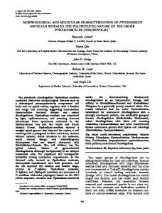
In the growth process, different growth rates were tried. It was found that lower growth rate usually leads to smooth surface. Typically, we used 0.1to0.2nm/sec. ITO surface was examined by using AFM. As shown in figure 5.1, ITO surface consists of small flakes, the surface roughness probably influences the device performance. In figure 5.2, the interface of Alq3 and the glass substrate is clearly shown. The upper part is Alq3, which looks like some kind of loose powder, the lower part is glass, which consists of many small humps.

33

34

CHAPTER 5. RESULTS AND DISCUSSIONS

Figure 5.1: Surface of ITO characterized by AFM

Figure 5.3 is the evidence of coevaporation of Al and Alq3. After the growth, Al cathode look very dark. And during Al deposition, only Al and Alq3 source were in the vacuum chamber. Checked by AFM, many clusters were found on the surface. So that I suspected it is the coevaporation of Al and Alq3. This coevaporation of Al and Alq3 provides lots of charge carrier traps, which leads to the failure of the device.

5.2

“Park” structure

In our project, “Park” structure device was grown in all nine kinds of chips. First, we are going to present the results of IV measurement of chip “ITO 060410BIII” to illustrate the electrical properties of the “Park” structure device. As we mentioned before, there are two types of ITO pattern for the BIII chips (see section 4.1 for pattern design), one is bar-shaped gate, the other is sawtoothshaped gate. So it is very interesting to explore the different performances caused by different patterns. In this chip, device 1 had the sawtooth-shaped gate, while device 4 had bar-shaped gate. The IV curves are shown in figures 5.4 and 5.5.

5.2. “PARK” STRUCTURE

Figure 5.2: Border of Alq3 and glass

Figure 5.3: Coevaporation of Al and Alq3

35

36

CHAPTER 5. RESULTS AND DISCUSSIONS

−4

5

ITO 060410BIII measure@060410 Device1

x 10

gate=−5 [V] gate=−10 [V] gate=−15 [V] gate=−20 [V]

4.5

4

3.5

ICA [A]

3

2.5

2

1.5

1

0.5

0

0

5

10

15

20

25

VCA [V]

Figure 5.4: IV curve of chip ITO 060410BIII Device 1 −5

5

ITO 060410BIII measure@060410 Device4

x 10

gate=−5 [V] gate=−10 [V] gate=−15 [V] gate=−20 [V]

4.5

4

3.5

ICA [A]

3

2.5

2

1.5

1

0.5

0

0

5

10

15

20

25

VCA [V]

Figure 5.5: IV curve of chip ITO 060410BIII Device 4

From these two figures, we may notice that the shape of the curves are quite similar, which indicates that they are from the same mechanism. However, we may also notice that the current in device 1 is one order of magnitude larger than the current of device 4. The same thing happened to other chips. The current of a device with sawtooth-shaped gate is usually larger than the current of a device

37

5.3. IV MEASUREMENT IN LIQUID NITROGEN

with bar-shaped gate. The reason for this phenomenon is unknown, the following is only our speculation. According to the pattern design, the edge of device with sawtooth-shape gate is longer than the device with bar-shape gate. And we know that the electrical field at the edge of the electrode is usually stronger than the middle part of electrode. This is because in the process of lithographic patterning, the etching rate is difficult to control. Consequently rough edges are commonly formed, which will lead to a strong electrical field as long as the voltage is applied. Combining the two reasons above, devices with sawtooth-shaped gate generates stronger electrical field, thus the current is larger. From figures, we see that the turn on voltage is around 10 V , which is in correspondence with the voltage when light-emitting starts. Another phenomenon is that when we carry out the IV measurement, the curve is always unsmoothed at the first time, so is the light emission. However, after applying voltage for two or three times, the curve turns normal. We suspect that it is a process of filling up traps during charge transport (see section 2.5.1). If no specific pointing out, all IV measurements are done by the following circuit (figure 5.6).

VCA V

C

VCG V G

A

A

keke

Figure 5.6: Circuit for the IV measurements

5.3

IV measurement in Liquid Nitrogen

For inorganic semiconductors, the crystal lattice will have less vibrations at low temperatures. Thus, the electron mobility will increases. Is it the same for organic semiconductors? In order to answer this question, we performed an IV measurement in liquid nitrogen.

38

CHAPTER 5. RESULTS AND DISCUSSIONS

The series number of the chip was “ITO 060407AII” with the structure: IT O/CuP C(11nm)/T P D(40nm)/ALq3(50nm)/Al(74nm). Liquid nitrogen were slowly poured into a plastic container after the device was connected to the outside circuit and placed correctly in the container. However, one corner of the device cracked due to thermal contraction. Luckily it did not affect the device performance. After the whole device was submerged in liquid nitrogen, we did IV measurements, and again 30 mins after the device was removed from the liquid nitrogen. It was room temperature by then. The two measurements are shown in figure 5.7.

IV curve measured at 23 °C and −196 °C

−4

9

x 10

8

at 23 °C at −196 °C

7

6

ICA [A]

5

4

3

2

1

0

−1 −5

0

5

10 VCA [V]

15

20

25

Figure 5.7: IV measurement did at 23℃ and -196℃

The curve in liquid nitrogen is flat in room temperature, which proved that the mechanism of charge transport for organic semiconductor is different from inorganic semiconductors. For small molecular semiconductors, hopping transport is the dominant mechanism. At lower temperature, charge carriers are more localized to individual molecule, instead of spreading out to several molecules. The thermal energy may be insufficient for charge carriers to overcome the barrier for hopping. Thus, the mobility of charge carriers is lower than at room temperature. Macroscopically, the current is lower, which shown in our experiment.

39

5.4. SPECTRAL MEASUREMENT

5.4

Spectral measurement

We used photo-luminescence to observe spectra from the device (Chip Series Number: ITO 060424BI). The results are shown in figure 5.8. The peak appears at approximately 535 nm, which is corresponding to the prediction from figure 3.1. According to device structure, the light is supposed to be emitted from the TPD/Alq3 interface. In the energy diagram, electrons from LUMO (3.3 eV) of Alq3 and holes from HOMO (5.6 eV) of TPD will be recombined somewhere in between. The energy difference from LUMO to HOMO converts to the photon energy, whose wavelength is: λ=

c hc 1240 = = = 539 nm ν ε 5.6 − 3.3

(5.1)

This is quite close to the measured result, 535 nm, which is in the range of green light. Besides, the shape of the spectra is not a series of sharp peaks, but a Gaussian-like distribution which confirmed that there are no well-defined band structure in organic semiconductors as we mentioned at the end of section 2.2.

Emission Spectra of Device 35

30

Intensity [arb. units]

25

20

15

10

5

0

440

460

480

500

520 540 560 Wavelength [nm]

580

600

620

640

Figure 5.8: PL-emission spectra of the device.(Many thanks to Ahmed Abdela and Petter Westbergh for the measurement.)

40

5.5

CHAPTER 5. RESULTS AND DISCUSSIONS

Degradation

During the spectral measurements, we observed a fast degradation of the device. This degradation is probably caused by Alq3 reacting with water and oxygen in the air. This is believed to be the main mechanism for the failure of the Alq3based devices[23, 24]. The Alq3 hydrolysis process is thermally activated. The final products, Alq2OH, were found responsible for causing the charge imbalance. Although, we tried to add a layer of silicone to protect the device. However, fast degradation still occurred. The device (Chip Series Number: ITO 060517CII) in figure 5.9 was measured directly in the air. Fitting shows that the intensity may be decreased exponentially. According to the definition of “lifetime” in display industrial, which is the time it takes when intensity of the device decreases to half of its original value, the lifetime of our device shown in this figure is approximately four hours. Besides, we tested with light on a device over night. After 17hours and 35 minutes, the emitted light was barely can be seen.

Measured Exponential fitting

Intensity [arb. units]

1400

1300

Data: intensity Model: ExpDec1 Equation: y = A1*exp(-x/t1) + y0 Weighting: y No weighting

1200

Chi^2/DoF = 187.97835 R^2 = 0.99079 y0 A1 t1

1100

834.65129 484.01395 37.95263

1000

900

800 0

20

40

60

80

100

Time [mins]

Figure 5.9: Degradation of device over time

5.6

Vertical OLET and horizontal OLET

Vertical OLET and horizontal OLET (see section 2.8) have different electrical characteristics. In order to compare them, we came up with the following IV measurements, shown in figure 5.10. The horizontal OLET (5.10(a)), and vertical OLET (5.10(b)). In the measurements, we set VCG to −15V, −10V, −5V, 0V, 5V, 10V, 15V

41

5.6. VERTICAL OLET AND HORIZONTAL OLET

respectively. For each VCG , we swept VCA from 0V to 20V . The currents that from the contacts are termed I1 , I2 and I3 . For simplicity, we did not grow multi organic layers on the ITO patterns. Instead a 105 nm thick TPD was grown with approximately 100 nm Al on top. This is the same thickness as a full structure device. Gate Organic layer(s) Cathode A2

Anode Substrate

A3

A1

VCG

VCA

(a) Horizontal OLET

Cathode Organic layer(s) Gate A3

Anode Substrate

A2 VCG

A1 VCA

(b) Vertical OLET

Figure 5.10: Horizontal OLET and vertical OLET In addition to the IV measurements, we made a circuit theory approach to derive general analytical equations for the cathode-anode current and cathode-gate current. In this simulation, we only considered bulk resistance of organic semiconductors, and ignored the contact resistance which simplified the system. This led to incompleteness of the approach. However, the simulation seems fitted the measured data.

5.6.1

Circuit theory approach

This circuit theory approach is base on the idea that the organic layers are three field-dependent resistances between the three electrods. In the setup 5.10(b) for example, the current I1 comes out from power supply VCA , I2 comes out from

42

CHAPTER 5. RESULTS AND DISCUSSIONS

power supply VCG , and I3 comes out from cathode. In figure 5.11, the resistances RCG , RAC and RGA represent organic layers between three electrodes.

C VCA

VCG

I3 RCG

RAC

I2 G I1

A

RGA

Figure 5.11: The organic layers are replaced with three resistors The three resistances form a typical “delta” circuit, which can be transformed to an “Y” circuit by the following relations:    RCO = RGO =   R AO =

RCG RAC RCG +RAC +RGA RCG RGA RCG +RAC +RGA RGA RAC RCG +RAC +RGA

(5.2)

The “Y” connection is shown below, in figure 5.12:

VCA

VCG I2

I3 RGO G

C RCO O

RAO A

I1 Figure 5.12: The “Y” connection circuit In order to see the circuit diagram more clearly, we identified the circuit 5.12 to 5.13, as shown below: Analyzing circuit 5.13, we may have the following relations: VCA (RCO + RGO ) − VCG RCO RCO RGO + RGO RAO + RAO RCO VCA (RCO + RGO ) − VCG RCO I2 = RCO RGO + RGO RAO + RAO RCO I1 =

(5.3a) (5.3b)

5.6. VERTICAL OLET AND HORIZONTAL OLET

A

43

RAO

I1 VCA

I3

C

RCO O

VCG I2

RGO

G

Figure 5.13: Final circuit

I3 = I1 + I2

(5.3c)

Combining equation 5.3 with the transformation relation equation 5.2, we get:

5.6.2

I1 =

VCA VCA VCG + − RCA RGA RGA

(5.4a)

I2 =

VCG VCG VCA + − RCG RGA RGA

(5.4b)

Field-dependent resistance

Now, we focus on the three resistance RCG , RCA and RGA . As everyone knows, the resistance R is proportional to the length of the resistor, L, and is inversely proportional to the cross-section area of the resistance A, that is L A And the resistivity in semiconductor has the relation of R=ρ·

ρ=

1 qnµ

(5.5)

(5.6)

Where, q is the elementary charge, n is the carrier concentration, µ is the fielddependent mobility[11]. As we mentioned in section 2.5, this field-dependent mobility is frequently observed in amorphous molecular materials. √ µ = µ0 exp(β E)

(5.7a)

q 3 1/2 1 ·( ) kT πεε0

(5.7b)

β=

44

CHAPTER 5. RESULTS AND DISCUSSIONS

Where, µ0 is zero-field mobility. Combining equations 5.5, 5.6 and 5.7, we get: R=

L qnµ0 exp(β

p

(5.8)

V /L)A

Each resistance has its corresponding L, V and A, which are distance, applied voltage, and intersection area between two electrodes respectively. Combining equations 5.4 and 5.8, we derived the expression for I1 and I2 as a function of VCA and VCG : r nqµ0 ACA VCA I1 = · exp(β ) · VCA LCA LCA r nqµ0 AGA VGA + · exp(β ) · VCA LGA LGA r nqµ0 AGA VGA · exp(β ) · VCG − LGA LGA

(5.9a)

r VCG nqµ0 ACG · exp(β ) · VCG I2 = LCG L rCG nqµ0 AGA VGA · exp(β ) · VCG + LGA LGA r nqµ0 AGA VGA − · exp(β ) · VCA LGA LGA

(5.9b)

VGA = VCA − VCG

(5.9c)

In equation 5.9, the parameters ACG , AGA , LCG and LGA are illustrated in the following figures, for the vertical structure:

Cathode LCG=LCA=105 nm ACG Gate

ACA AGA

Anode LGA=30 um

Figure 5.14: For the horizontal structure we have:

45

5.6. VERTICAL OLET AND HORIZONTAL OLET

Gate LCG=LGA=105 nm ACG

AGA ACA

Cathode

Anode LCA=30 um

Figure 5.15:

5.6.3

Curve fitting

5 CA AGA In our case (Chip Series Number: ITO 060721BIII), the value of A LCA / LGA ≈ 10 and together with the additional condition that VCG = 0, we can ignore the second and third terms in equation 5.9a, and simplify it to:

nqµ0 ACA I1 = · exp(β LCA

r

VCA ) · VCA LCA

(5.10)

In equation 5.10, the parameters L, A and V are known, but two parameters nqµ0 and β are still unknown. In order to find them, we picked up one I1 VS VCA curve, measured at VCG = 0, and fitted into equation 5.10. The fitting process was made by the software Origin 7.5, and the results are shown in figure 5.16.

Data: Data1_B Model: oled Weighting: y No weighting

0.00004

Measured data Simulated data

Chi^2/DoF = 2.0189E-13 R^2 = 0.99802 c b

ICA [A]

0.00003

7.6687E-13 0.00074

¡ À 1.1435E-13 ¡ À 0.00001

0.00002

0.00001

0.00000

-2

0

2

4

6

8

10

12

14

VCA [V]

Figure 5.16: IV curve fitting

16

18

20

22

46

CHAPTER 5. RESULTS AND DISCUSSIONS

In this figure, the two parameters were found to be following values: nqµ0 = 7.6687 × 10−13 , and β = 7.4 × 10−4 .

5.6.4

Simulation and comparison of horizontal OLET and vertical OLET

Using the values obtained from previous section and using equation 5.9, we simulated I1 and I2 at different VCG and compared them with experimental data. The matlab codes are given in appendix C. The results are shown in the figures 5.17 to 5.20. In these figures, we can see that the simulated results fit quite well to measured ones. Figure 5.17 shows the results of the vertical OLET with positive gate bias. The cathode-gate and cathode-anode structure actually form two parallel OLEDs. In this case, both simulated and measured IV curves overlap each other, which means that the cathode-anode bias current I1 is not controlled by the gate. The observed leakage current I2 is quite high and is controlled by the gate. However, in few cases, the cathode-anode bias current was controlled by the gate, but the reason for that is not clear. In figure 5.18, the results from a vertical OLET, with negative gate bias, are shown. The leakage current we observed to be very low. In this case, the cathodegate forms an inverse OLED, which provides high injection barrier for the holes at the interface of cathode and organic layers. The results show that the IV curves CA were weakly controlled by the gate. In the simulation, when the value of A LCA AGA and LGA are close, gate shows good controlling ability (see figure 5.14). So we conclude that this gate control could be improved by shrinking the gate-anode channel length. Figure 5.19 shows the results from a horizontal OLET with positive gate bias. We observed the bias current is controlled by the gate. A relatively low leakage current was also observed. This is due to the reason of forming inverse OLED by gate and anode, the same as the vertical OLET with negative gate bias we stated few paragraphs before. In figure 5.20, we have negative gate bias applied on horizontal OLET. In this case, the leakage current is quite high. The IV curve shift is due to this leakage current. The solution is to add an insulator layer between the top gate and organic layers. In summary, due to the high leakage current, we abandoned the positive gate

47

5.6. VERTICAL OLET AND HORIZONTAL OLET

−5

4.5

Vertical OLET with positive gate voltage

x 10

Measured data

4

Simulated max I2 at VCG=15 V 3.5

Simulated I1

3

I1 [A]

2.5

2

1.5

1

0.5

0

0

2

4

6

8

10 VCA [V]

12

14

16

18

20

Figure 5.17: Vertical OLET with positive VCG

−5

4.5

Vertical OLET with negative gate voltage

x 10

Measured data

4

Simulated max I2 at VCG=−15 V 3.5

Simulated I1

3

I1 [A]

2.5

2

1.5

1

0.5

0

0

2

4

6

8

10 VCA [V]

12

14

16

18

Figure 5.18: Vertical OLET with negative VCG

20

48

CHAPTER 5. RESULTS AND DISCUSSIONS

−5

4.5

Horizontal OLET with positive gate voltage

x 10

Measured data

4

Simulated max I2 at VCG=15 V 3.5

Simulated I1

3

I1 [A]

2.5

2

1.5

1

0.5

0

0

2

4

6

8

10 VCA [V]

12

14

16

18

20

Figure 5.19: Horizontal OLET with positive VCG

−4

10

Horizontal OLET with negative gate voltage

x 10

Measured data Simulated max I2 at VCG=−15 V

8

Simulated I1

I1 [A]

6

4

2

0

0

2

4

6

8

10 VCA [V]

12

14

16

18

Figure 5.20: Horizontal OLET with negative VCG

20

5.7. “KUDO STRUCTURE”, THE DISCONTINUOUS FILM

49

bias for the vertical OLET and the negative gate bias for horizontal OLET. In addition we should pay more attention on the vertical OLET with negative gate bias and the horizontal OLET with positive gate bias.

5.7

“Kudo structure”, the discontinuous film

In the “Kudo” structure, we tried a discontinuous film instead of using a mask for deposition of a metal film grid. A discontinuous Al film was deposited on a glass substrate and the resistance of the film was measured. AFM imagine of such films are shown in figure 5.21. During the process of Al deposition, the Al film first formed small islands, which merges to big islands and finally formed continuous film. Our purpose was to find the thickness somewhere between forming islands and a continuous film, where Al forms discontinuous film. In figure 5.21(b) and (c), the resistances are infinite and 8.15 × 109 Ω respectively, which means it is probably Al islands on glass. In (d) the resistance was 161 Ω, and we know that the resistance of bulk Al is around 0.3 Ω, so that the thickness of discontinuous film is probably slightly thicker than 5 nm. We also grown a device with 5 nm discontinuous film in organic layers. The IV curve are shown in figure 5.22. From this figure, the IV curve is shifted at different gate voltages. But to 100 percent sure the device is working, we need more experiments and optimization.

50

CHAPTER 5. RESULTS AND DISCUSSIONS

Figure 5.21: Al discontinuous film with different thickness deposited on the glass substrates:(a) The glass substrate with the RMS roughness 0.74 nm; (b) 2 nm of Al deposited with a roughness of 0.25 nm, and infinite resistance; (c) 3.5 nm of Al deposited with the roughness 1.16 nm, and resistance of 8.15×109 Ω; and finally (d) 5 nm of Al deposited with the roughness 1.75 nm, and resistance of 161 Ω

51

5.7. “KUDO STRUCTURE”, THE DISCONTINUOUS FILM

−3

8

Kudo Structure 060517CII

x 10

Gate= 0 [V] Gate=05 [V] Gate=10 [V] Gate=15 [V]

7

6

ICA [A]

5

4

3

2

1

0

−1

0

1

2

3

4

5 VCA [V]

6

7

8

9

Figure 5.22: IV curve of a device with a discontinuous film.

10

Chapter 6

Future work In this diploma work, three kind of organic light-emitting transistors were fabricated, which are “Park” structure of vertical OLET, top contact structure of horizontal OLET and “Kudo” structure with discontinuous film. And their electrical properties and optical properties were characterized by IV measurement system and photoluminescence spectrometer, the surfaces of organic semiconductors used in this work were examined by atomic force microscopy. Finally, light-emitting was achieved in this work, and gate electrode shows controlling ability in some devices.

Figure 6.1: A device successfully emit light The above figure shows a device that successfully emits light. However, there are

53

54

CHAPTER 6. FUTURE WORK

still problems which needs to be solved and many aspects could be improved. For instance, our growth pressure is around 4 × 10−6 mbar, if we can achieve higher vacuum, the device quality could be better. The device performance could also improved by using other low work function metal as cathode, for example Mg/Ag alloy. Another big problem is the degradation of the device, as we mentioned before the main mechanism is the reaction of Alq3, water and oxygen. There two way to solve this. One is to find less active materials that could replace Alq3, the other is to develop efficient encapsulation layer that could protect Alq3. Currently, the degradation of Alq3 is the main obstacle for doing more measurements. We did IV measurements both in vertical OLET and horizontal OLET. The gate controlling of vertical OLET could be improved by shrinking the gate-anode channel length. And the gate controlling of horizontal OLET is better. The high leakage current could be avoided by adding an insulator layer. In the device simulation, we only considered bulk resistance. If the contact resistance was considered, the deviation of simulated results could be smaller. Also, more experiments in low temperature should be carried out to investigate the basic rules of the charge transport process.

Bibliography

[1]

A.Bernanose. Electroluminescence of organic compounds. Brit. J. Appl. Phys. Suppl., 4(S54), 1955. [cited at p. 1]

[2]

P.Magnante M.Pope, H.Kallmann. Electroluminescence in organic crystals. J. Chem. Phys., 38(2042), 1963. [cited at p. 1]

[3]

W.G.Schneider W.Helfrich. Recombination radiation in anthracene crystals. Phys. Rev. Lett., 140(229), 1965. [cited at p. 1]

[4]

C.W.Tang and S.A.VanSlyke. Organic electroluminescent diodes. Appl. Phys. Lett., 51(913), 1987. [cited at p. 1, 15, 79]

[5]

G.Grosso(Edr.) R.Farchioni. Organic Electronic Materials. Springer, 2001. [cited at p. 5]

[6]

Bart Van Zeghbroeck. Principles of Semiconductor Devices. Internet, http://ece-www.colorado.edu/˜bart/book/book/title.htm, 2004. [cited at p. 7]

[7]

Y.H.Tak H.Bassler V.I.Arkhipov, E.V.Emelianova. Charge injection into light-emitting diodes: Theory and experiment. J. Appl. Phys., 84(848), 1998. [cited at p. 9]

[8]

H.Bassler U.Wolf, V.I.Arkhipov. Current injection from a metal to a disordered hopping system. i montecarlo simulation. Phys. Rev. B, 59(7507), 1999. [cited at p. 9]

[9]

David Lidzey. Organic semiconductors and devices. [cited at p. 10]

[10] R.W.Gurney N.F.Mott. Electronic Processes in Ionic Crystals. Clarendon Press, Oxford, 1940. [cited at p. 10] [11] P.N.Murgatroyd. Theory of space-charge limited current enhanced by frenkel effect. J. Phys. D: Appl. Phys., 3(151), 1970. [cited at p. 10, 43]

55

56

BIBLIOGRAPHY

[12] Jan Kalinowski. Electroluminescence in organics. J. Phys. D: Appl. Phys., 32:R179–R250, 1999. [cited at p. 12] [13] Anton G.Muckl Wolfgang Brutting, Stefan Berleb. Device physics of organic light-emitting diodes based on molecular materials. Organic Electronics, 2:1– 36, 2001. [cited at p. 12] [14] Mauro Murgia Siegfried Karg Walter Riess Maria Antonietta Loi, Constance Rost-Bietsch and Michele Muccini. Tuning optoelectronic properties of ambipolar organic light-emitting transistors using a bulk-heterojunction approach. Adv. Funct. Mater., 16:41–47, 2006. [cited at p. 16, 79] [15] Chihaya Adachi Suguru Okuyama Noriyuki Shimoji Takahito Oyamada, Hi0 royuki Sasabe and Kazumi Matsushige. Electroluminescence of 2,4-bis(4-(2 thiophene-yl)phenyl)thiophene in organic light-emitting field-effect transistors. Appl. Phys. Lett., 86(093505), 2005. [cited at p. 16, 79] [16] M.A.Loi M.Murgia F.Cicoira V.A.L.Roy P.Stallinga R.Zamboni C.Rost S.F.Karg C.Santato, R.Capelli and M.Muccini. Tetracene-based organic light-emitting transistors: optoelectronic properties and electron injection mechanism. Synthetic Metals, 146:329–334, 2004. [cited at p. 16] [17] Wieland Weise Marcus Ahles Roland Schmechel Aline Hepp, Holger Heil and Heinz von Seggern. Light-emitting field-effect transistor based on a tetrancene thin film. Phys. Rev. Lett., 91(15), 2003. [cited at p. 16] [18] Byoungchoo Park and Hideo Takezoe. Enhanced luminescence in topgate-type organic light-emitting transistors. Appl. Phys. Lett., 85(7), 2004. [cited at p. 16, 25]

[19] Masaaki Iizuka Kazuhiro Kudo, Satoshi Tanaka and Masakazu Nakamura. Fabrication and device characterization of organic light emitting transistors. Thin Solid Films, 438-439:330–333, 2003. [cited at p. 17, 25] [20] http://en.wikipedia.org/wiki/Indium tin oxide. [cited at p. 19] [21] http://www.alfa.com. [cited at p. 21] [22] http://www.sigmaaldrich.com.com. [cited at p. 21, 22] [23] Nan-Xing Hu Ah-Mee Hor Gu Xu Hany Aziz, Zoran D.Popovic. Degradation mechanism of small molecule-based organic light-emitting devices. Science, 283:1900–1902, March 1999. [cited at p. 23, 40] [24] Hrant P.Hratchian H.Bernhard Schlegel John E.Knox, Mathew D.Halls. Chemical failure modes of alq3-based oleds: Alq3 hydrolysis. Physical Chemistry Chemical Physics, 8:1371–1377, 2006. [cited at p. 23, 40]

57

[25] Qiang Huang. Growth of Organic Materials for Light Emitting Device. PhD thesis, Chalmers University of Technology, 2003. [cited at p. 23, 25] [26] Borge Wessling. Electrical Behavior, Degradation and Equivalent Circuits of Organic Light Emitting Diodes Based on Small Molecules. PhD thesis, Chalmers University of Technology, 2004. [cited at p. 25] [27] Michael Wank. Growth and Characterization of Doped Organic Semiconductor LED Heterostructures. PhD thesis, Chalmers University of Technology, 2004. [cited at p. 25] [28] Saˇsa Vuˇckovi´c. Modeling and Fabrication of Organic Semiconductor Light Emitting Transistors. PhD thesis, Chalmers University of Technology, 2005. [cited at p. 25]

[29] Ahmed Abdela and Petter Westbergh. Fabrication and characterization or organic transistors. Technical report, Chalmers University of Technology, 2006. [cited at p. 25] [30] Milton Ohring. Materials Science of Thin Films - Deposition and Structure. Academic Press, second edition, 2002. [cited at p. 27] [31] http://www.lesker.com. [cited at p. 61]

Appendices

59

Appendix A

Estimate the temperature of tungsten heater in vacuum

For aluminum deposition, we used a PBN crucible as the aluminum source which sit in a tungsten basket heater. Therefore, it is useful to estimate the temperature of the tungsten heater versus the current that go through the wire. In the experiment, there are two kinds of tungsten basket heater suitable for the PBN crucible, which is purchased at Kurt J. Lesker [31] through internet. One heater is with diameter of 0.025 inches (Part No. EVB8A3025W), the other is with diameter of 0.030 inches (Part No. EVB8A3030W). Normally, the heat could be transferred by conduction, convection and radiation. In our case, the heater is placed in vacuum, so that, heat convection is no longer available. Thus heat is mainly transferred in the form of radiation, and a small proportion of the heat is transferred by phonon vibrations of contacts. The radiation in vacuum follows Stefan-Boltzmann’s Law, which is described by the following equation: P = σ · ² · A · T4

(A.1)

Where P is the radiant power, 2π 5 k4 −8 Js−1 m2 K 4 , σ is Stefan-Boltzmann constant, σ = 15c 2 h3 = 5.67 × 10 ² is the emissivity, for tungsten ² ≈ 0.23 K −1 , A is the surface area of the tungsten wire, T is the temperature in unit of Kelvin. Suppose the supplied power is completely converted to radiant power, then we

61

APPENDIX A. ESTIMATE THE TEMPERATURE OF TUNGSTEN HEATER IN VACUUM

62

have the following equation: I 2R = σ · ² · A · T 4

(A.2)

The resistance is: R=ρ·

L 4L = ρ0 · [1 + α(T − T0 )] · 3πd2 A0

(A.3)

By combining equation (A.2) and (A.3), we have: 4L = σ · ² · 3π · d · L · T 4 (A.4) πd2 Where, ρ0 is the resistivity at T0 , d is the diameter of the thread, α is the temperature coefficient. By solving this equation (A.4), we get T = f (I, d). I 2 · ρ0 [1 + α(T − T0 )] ·

Consider a real case, for example, in our experiment with tungsten wire, we have these parameters: ρ0 = 5.65 · 10−8 Ωm σ = 5.67 · 10−8 Js−1 m2 K 4 ² = 0.23 K −1 α = 4.83 · 10−3 K −1 T0 = 300 K L = 1m So, by calculation, we get table A.1. H

HH

d

H

I

20 30 40 50 60 70

HH H

[A] [A] [A] [A] [A] [A]

0.025˝

0.030˝

832 ℃ 1185 ℃ 1500 ℃ 1790 ℃ 2061 ℃ 2318 ℃

642 ℃ 936 ℃ 1200 ℃ 1441 ℃ 1667 ℃ 1880 ℃

Table A.1: Temperature as a function of the current for two different wire diameters It is quite clearly that 0.025 inches (0.635 mm) heater is better than 0.030 in (0.762 mm) heater, because for the same current, 0.025 inches heater generates more heat. That is to say, we can achieve the same temperature at a lower current, which will greatly increase the lifetime∗ of tungsten basket heater. After ∗

Normally, the lifetime of a 0.030 inches tungsten wire is around 3 weeks, considering 4 rounds of growth per week and 30 mins per round.

63

several rounds of deposition at high current, the tungsten heater becomes very brittle. Even to remove it from the contact arms will possibly break it. So that it was much better to run it at a low current. However, when I was working on this diploma work, the 0.025 inches heater was run out, so, all the aluminum deposition was done using 0.030 inches heater.

Appendix B

Procedure of cleaning, pumping, growth and measurements

B.1

Cleaning procedure

Before growing any devices, the substrates must be cleaned. Borrowing the experience from the inorganic semiconductor part of this group, we developed a procedure of substrates cleaning as follow: 1. Warming-up ultrasonic bath for 10 mins. 2. Clean with Tri or equivalent in ultrasonic bath for 15 mins. 3. Clean with Acetone in ultrasonic bath for 15 mins. 4. Clean with Methanol in ultrasonic bath for 15 mins. 5. Rinse with deionized water. 6. Dry with N2 gas.

B.2 B.2.1

Pumping procedure Pumping down

1. Turn on the cooling water. 2. Put the Valve to position 2 and switch on the rotary pump to pump the diffusion pump.

65

APPENDIX B. PROCEDURE OF CLEANING, PUMPING, GROWTH AND MEASUREMENTS

66

Vacuum Chamber On-Off

TPR2

0

3

3 2 1

0

Valves 1

Diffusion Pump TPR1 Cooling Water 2

Rotary Pump

Figure B.1: Sketch of bell jar vacuum system 3. After TPR1 is below 30 mtorr, switch on the diffusion pump and let it warm up for 15 mins. 4. Check so “on-off” is closed, put the Valve to 1, so rotary pump is rough pumping the vacuum chamber. 5. It probably takes 8 mins for TPR2 to reach 10−1 mbar by the rotary pump. 6. Check so TPR2 is below 10−1 mbar and TPR1 is below 30 mtorr. If not, repeat 2 and 4. 7. Put the Valve to 3 for the diffusion pump to pump the vacuum chamber. 8. When TPR2 has reached 10−6 mbar, the vacuum is ready for deposition. The total time of this is around 1 hour.

B.2.2

Breaking the vacuum

1. Turn the Valve to 0 and after this open “on-off” to let in air or nitrogen gas. 2. Remove or change your sample and remount the bell jar. 3. Close the “on-off” valve and put the Valve to 2. 4. Pump down again or turn off the system.

B.3. GROWTH PROCEDURE OF THE “PARK STRUCTURE”

B.2.3

67

Turning off the system

1. If it is desired to take out the sample, then open “on-off” to let in air. 2. Take out sample. 3. Switch off the diffusion pump. 4. Put the Valve to 2. 5. Leave the rotary pump to pump the diffusion pump for 10 mins. 6. Switch off the rotary pump. 7. Leave the cooling water to continue to run for ∼20 mins. Check that if it is warm, if not, turn off the cooling water and put Valve back to position 1.

Notice: As long as the diffusion pump is running, the cooling water MUST be on and the diffusion pump can not work at low vacuum for long time, say several hours.

B.3

Growth procedure of the “Park structure”

CuPc, 15 nm 1. Set CuPc’s density (1.64 GM/CC) on the thickness monitor. 2. Attach the cables to the CuPc source’s copper rods. 3. Turn on the power supply. 4. 0 min - turn the knob to 10 V (4 A). 5. 5 min - turn the knob to 20 V (10 A). 6. 10 min - turn the knob to 27 V (12 A). 7. Start monitoring the deposition rate. 8. Remove the shutter, set total thickness to 0 nm on the thickness monitor and start the deposition when the desired rate is stable. 9. Move back the shutter when the desired layer thickness, say 15 nm is achieved. The deposition takes about 75 secs when the deposition rate is 2 ˚ A/sec.

APPENDIX B. PROCEDURE OF CLEANING, PUMPING, GROWTH AND MEASUREMENTS

68

10. Slowly turn back the knob to 0. 11. Shut down the power supply. 12. Wait 10 minutes to cool down in the vacuum chamber before evaporation from next source. TPD, 40 nm 1. Change to TPD’s density (1.6 GM/CC) on the thickness monitor. 2. Attach the cables to the TPD source’s copper rods 3. Turn on the power supply. 4. 0 min - turn knob to 10 V (3 A). 5. 5 min - turn knob to 13 V (5 A). 6. 10 min - turn knob to 14 V (5 + A). 7. Start monitoring the deposition rate. 8. Move shutter and start deposition when the desired rate is stable. 9. Move back the shutter when the desired layer thickness is achieved. 10. Slowly turn back the knob. 11. Shut down the power supply. 12. Wait 10 minutes before evaporation of next source. Alq3, 50 nm 1. Change to Alq3’s density (1.4 GM/CC) in the thickness monitor. 2. Attach the cables to the Alq3 source’s copper rods 3. Turn on the power supply. 4. 0 min - turn knob to 15 V (2 A). 5. 5 min - turn knob to 19 V (3 − A). 6. 10 min - turn knob to 21 V (3 + A). 7. Start monitoring the deposition rate. 8. Move shutter and start deposition when the desired rate is stable. 9. Move back the shutter when the desired layer thickness is achieved.

B.4. IV MEASUREMENT PROCEDURE

69

10. Slowly turn back the knob. 11. Shut down the power supply. 12. Wait 10 minutes before evaporation from next source. Al, 70-100 nm 1. Change to Al’s density (2.7 GM/CC) on the thickness monitor. 2. Attach the cables to the Al source’s copper rods 3. Turn on the power supply. 4. 0 min - turn knob to 10 V (14 A). 5. 5 min - turn knob to 20 V (22 A). 6. 10 min - turn knob to 30 V (30 A). 7. 15 min - turn knob to 40 V (36 A). 8. 20 min - turn knob to 50 V (44 A). 9. 25 min - slowly increase the voltage and monitoring the deposition rate, the current should below 70 A. 10. Move the shutter and start deposition when the desired rate is stable. 11. Move back the shutter when the desired layer thickness is achieved. 12. Decrease the voltage in the pace of 10 V /2 mins, until the voltage is 0. 13. Shut down the power supply. 14. Wait 20 minutes for cooling before breaking the vacuum.

B.4

IV measurement procedure

The circuit connections are discussed in section 4.5, here we just give the standard measurement procedure. 1. Sweep VCA starting from −5 V to 25 V in steps of 0.5 V . 2. Make sweep for VCG = 0, −1, −3, −5, −10, −15, −20, −25 V . Note that if the polarity of the voltage supply is changed, VCG should be the corresponding plus numbers.

Appendix C

Matlab code of processing IV measurement data This is an example of using matlab for processing IV measurement data. s1g00 s1g05 s1g10 s1g15

= = = =

dlmread(’S1vcg00_vca0_0.5_25.txt’,’,’,2,0); dlmread(’S1vcg05_vca0_0.5_25.txt’,’,’,2,0); dlmread(’S1vcg10_vca0_0.5_25.txt’,’,’,2,0); dlmread(’S1vcg15_vca0_0.5_25.txt’,’,’,2,0);

s1g00=s1g00(1:31,:);s1g00(:,2)=-s1g00(:,2); s1g05=s1g05(1:31,:);s1g05(:,2)=-s1g05(:,2); s1g10=s1g10(1:31,:);s1g10(:,2)=-s1g10(:,2); s1g15=s1g15(1:31,:);s1g15(:,2)=-s1g15(:,2); plot(s1g00(:,1),s1g00(:,2),’ks’) hold on; plot(s1g05(:,1),s1g05(:,2),’ks’) plot(s1g10(:,1),s1g10(:,2),’ks’) plot(s1g15(:,1),s1g15(:,2),’ks’) text(max(s1g00(:,1)),max(s1g00(:,2)),’\leftarrow------- m0’,’BackgroundColo r’,’w’) text(max(s1g05(:,1)),max(s1g05(:,2)),’\leftarrow------- m5’,’BackgroundColo r’,’w’) text(max(s1g10(:,1)),max(s1g10(:,2)+0.1e-5),’\leftarrow------- m10’,’Backgr oundColor’,’w’) text(max(s1g15(:,1)),max(s1g15(:,2)),’\leftarrow------- m15’,’BackgroundCol

71

72

APPENDIX C. MATLAB CODE OF PROCESSING IV MEASUREMENT DATA or’,’w’)

c=7.0193e-12; b=6.5e-4; Vac=0:0.1:15; Vgc=[0 5 10 15]; %S1 Aac=16e-6*30/39; Lac=105e-9; Aga=100e-9*2e-3*40; Lga=30e-6; Agc=16e-6*3/39; Lgc=105e-9; i=1; Vga=Vac-Vgc(i); I1=c*exp(b*sqrt(Vac./Lac)).*Aac.*Vac./Lac+c*exp(b*sqrt(Vga./Lga)).*Aga.*Vac ./Lga-c*exp(b*sqrt(Vga./Lga)).*Aga.*Vgc(i)./Lga; plot(Vac,I1); text(max(Vac),max(I1),’\leftarrow 0’,’Color’,’b’) i=2; Vga=Vac-Vgc(i); I1=c*exp(b*sqrt(Vac./Lac)).*Aac.*Vac./Lac+c*exp(b*sqrt(Vga./Lga)).*Aga.*Vac ./Lga-c*exp(b*sqrt(Vga./Lga)).*Aga.*Vgc(i)./Lga; plot(Vac,I1); text(max(Vac),max(I1),’\leftarrow 5’,’Color’,’b’) i=3; Vga=Vac-Vgc(i); I1=c*exp(b*sqrt(Vac./Lac)).*Aac.*Vac./Lac+c*exp(b*sqrt(Vga./Lga)).*Aga.*Vac ./Lga-c*exp(b*sqrt(Vga./Lga)).*Aga.*Vgc(i)./Lga; plot(Vac,I1); text(max(Vac),max(I1),’\leftarrow 10’,’Color’,’b’) i=4; Vga=Vac-Vgc(i); I1=c*exp(b*sqrt(Vac./Lac)).*Aac.*Vac./Lac+c*exp(b*sqrt(Vga./Lga)).*Aga.*Vac ./Lga-c*exp(b*sqrt(Vga./Lga)).*Aga.*Vgc(i)./Lga;

73

I2=c*exp(b*sqrt(Vgc(i)./Lgc)).*Agc.*Vgc(i)./Lgc+c*exp(b*sqrt(Vga./Lga)) .*Aga.*Vgc(i)./Lga-c*exp(b*sqrt(Vga./Lga)).*Aga.*Vac./Lga; plot(Vac,I1); text(max(Vac),max(I1),’\leftarrow 15’,’Color’,’b’) title(’[S1] Side gate with plus gate voltage’) xlabel(’V_{CA} [V]’) ylabel(’I_{1} [A]’) grid on; axis([0 20 -0.5e-5 3e-5]) print -deps ’sim_S1’

Appendix D

Shadow width as function of mask position

The appendix is the calibration of the wire mask. This work is done at the first of the diploma work for training of using the bell jar system. For the bell jar system please see section 4.2 and figure 4.2. The follow figure D.1 is showing the relative position of evaporation source (the blue box), wire mask (the circle) and substrate (the white box). When heating the source, the evaporant were blocked by the wire mask and leave a clear ribbon with width of d in the substrate. Our objective is to find how the width d as function of distance between substrate and mask. Figure D.2 is a close look of the mask. By calculation, we get the following results: (a2 − 2ar1 + r12 − r22 )(z1 + z2 ) p (a − r1 )z2 − r22 (a2 − 2ar1 + r12 − r22 + z22 ) (a2 + 2ar1 + r12 − r22 )(z1 + z2 ) p − (a + r1 )z2 + r22 (a2 + 2ar1 + r12 − r22 + z22 )

d = 2r1 +

(D.1)

Where, as indicated in figure D.1, z1 is the distance between mask and substrate, z2 is the distance between source and mask, and here z1 + z2 = 202 mm, r1 = 5 mm which is the radius of the evaporation crucible, r2 = 62.5 × 10−3 mm which is the radius of the wire of mask, d is the channel width, a = 85 mm which is the distance between the center of source and center of the wire. Besides calculation, we also measured the channel width. Both of the results are showed in figure D.3. It shows that the measured results are shifted about 40 µm up from the calculated ones, which I suspect is the error originated from blur edges as showed in figure D.4.

75

76 APPENDIX D. SHADOW WIDTH AS FUNCTION OF MASK POSITION

substrate d wire

z1

r2 evaporation beam z2

r1

evaporation source a

Figure D.1: Sketch of evaporation system

Figure D.2: Mask with wires of 125 µm width

77

Channel width as function of distance between substrate and mask 175 Calculated Measured 150

Channel width [µm]

125

100

75

50

25

0

0

0.5

1 1.5 2 2.5 Distance between substrate and mask [mm]

3

3.5

Figure D.3: Channel width as function of distance between substrate and mask

Figure D.4: An example of blur edge

List of Figures

2.1 2.2 2.3 2.4 2.5

Energy diagram of metal, semiconductor and insulator . . . . . . . . . sp2 hybridization (This graph is mosaiced due to the issue of copyright.) Splitting of π bond to LUMO and HOMO . . . . . . . . . . . . . . . . Three tunneling mechanisms at a metal-semiconductor interface . . . Charge carrier mobility in TPD and Alq3 obtained by TOF technique by different authors (This graph is mosaiced due to the issue of copyright.) . . . . . . . . . . . . . . . . . . . . . . . . . . . . . . . . . . . . 2.6 Sketch of traps in organic semiconductors: electrons and their directions are indicated by dots with arrows; the dashed circle indicates a trap, which electrons fall in. When the traps are filled, mobility increases in certain amount. . . . . . . . . . . . . . . . . . . . . . . . 2.7 Classification scheme of the EL phenomenon (This graph is mosaiced due to the issue of copyright.) . . . . . . . . . . . . . . . . . . . . . . 2.8 Basic steps of EL in organic: À charge carrier injection, Á charge carrier transport, Â exciton formation, Ã radiative exciton decay. Polaronic effects and a distribution of transport states due to disorder are neglected. (ΦA : anode work function, ΦC : cathode work function, Φh : hole injection barrier, Φc : electron injection barrier, Φbi : built-in potential, V : applied voltage, V : effective voltage across the organic layer, q: elementary charge) (This graph is mosaiced due to the issue of copyright.) . . . . . . . . . . . . . . . . . . . . . . . . . . . . . . . . 2.9 Top and Side view of the substrate holder. The chip dimension is based on this substrate holder. . . . . . . . . . . . . . . . . . . . . . . 2.10 Sketch of the chip CIII: the substrate is glass with the ITO pattern separated to left half and right half. . . . . . . . . . . . . . . . . . . . . 2.11 Basic structure of OLED[4] . . . . . . . . . . . . . . . . . . . . . . . . 2.12 Two types of horizontal OLET: (a) Bottom contact, (b) Top contact. The circle near cathode is the carrier recombination and exciton formation region.[14, 15] . . . . . . . . . . . . . . . . . . . . . . . . . . .

79

4 4 4 7

9

11 12

14 14 15 15

16

80

List of Figures

2.13 Two types of vertical OLET: (a) “Park structure” with anode and gate ITO pattern on the substrate, (b) “Kudo structure” with net shaped gate stretch into organic layers . . . . . . . . . . . . . . . . . . 17 3.1 3.2 3.3 3.4

Energy level diagram for some materials . . . Molecular structure of CuPc . . . . . . . . . Molecular structures of TPD and NPB . . . Molecular structures of Alq3 and PyPySPyPy

4.1

(a): Not fully etched ITO will cause short circuit of anode and gate; (b): Over etched ITO decrease electric field in organic layers . . . . Layout of deposition system and monitors: (1) thickness sensor, (2) shutter, (3) substrate holder, (4) mask holder, (5) thickness monitor, (6) diffusion pump pressure gauge, (7) vacuum chamber pressure gauge, (8) position of TPD source, (9) position of CuPc source, (10) position of Alq3 source, (11) position of Al source . . . . . . . . . . Circuit diagram to measure IV characteristics of the “Park structure” chips. . . . . . . . . . . . . . . . . . . . . . . . . . . . . . . . . . . . Sketch of Atomic Force Microscopy.(Many thanks to Yichen Zhang for sketching this graph.) . . . . . . . . . . . . . . . . . . . . . . . .

4.2

4.3 4.4

5.1 5.2 5.3 5.4 5.5 5.6 5.7 5.8 5.9 5.10 5.11 5.12 5.13 5.14 5.15 5.16 5.17 5.18 5.19 5.20

. . . .

. . . .

. . . .

. . . .

. . . .

. . . .

. . . .

. . . .

. . . .

. . . .

. . . .

. . . .

. . . .

Surface of ITO characterized by AFM . . . . . . . . . . . . . . . . . Border of Alq3 and glass . . . . . . . . . . . . . . . . . . . . . . . . Coevaporation of Al and Alq3 . . . . . . . . . . . . . . . . . . . . . . IV curve of chip ITO 060410BIII Device 1 . . . . . . . . . . . . . . IV curve of chip ITO 060410BIII Device 4 . . . . . . . . . . . . . . Circuit for the IV measurements . . . . . . . . . . . . . . . . . . . . IV measurement did at 23℃ and -196℃ . . . . . . . . . . . . . . . PL-emission spectra of the device.(Many thanks to Ahmed Abdela and Petter Westbergh for the measurement.) . . . . . . . . . . . . . . . . Degradation of device over time . . . . . . . . . . . . . . . . . . . . Horizontal OLET and vertical OLET . . . . . . . . . . . . . . . . . The organic layers are replaced with three resistors . . . . . . . . . . The “Y” connection circuit . . . . . . . . . . . . . . . . . . . . . . . Final circuit . . . . . . . . . . . . . . . . . . . . . . . . . . . . . . . . . . . . . . . . . . . . . . . . . . . . . . . . . . . . . . . . . . . . . . . . . . . . . . . . . . . . . . . . . . . . . . . . . . . . . . . . . . . IV curve fitting . . . . . . . . . . . . . . . . . . . . . . . . . . . . . . Vertical OLET with positive VCG . . . . . . . . . . . . . . . . . . . . Vertical OLET with negative VCG . . . . . . . . . . . . . . . . . . . Horizontal OLET with positive VCG . . . . . . . . . . . . . . . . . . Horizontal OLET with negative VCG . . . . . . . . . . . . . . . . . .

. . . .

21 22 22 23

. 26

. 28 . 30 . 31 . . . . . . .

34 35 35 36 36 37 38

. . . . . . . . . . . . .

39 40 41 42 42 43 44 45 45 47 47 48 48

81

List of Figures

5.21 Al discontinuous film with different thickness deposited on the glass substrates:(a) The glass substrate with the RMS roughness 0.74 nm; (b) 2 nm of Al deposited with a roughness of 0.25 nm, and infinite resistance; (c) 3.5 nm of Al deposited with the roughness 1.16 nm, and resistance of 8.15 × 109 Ω; and finally (d) 5 nm of Al deposited with the roughness 1.75 nm, and resistance of 161 Ω . . . . . . . . . . 50 5.22 IV curve of a device with a discontinuous film. . . . . . . . . . . . . . 51 6.1

A device successfully emit light . . . . . . . . . . . . . . . . . . . . . . 53

B.1 Sketch of bell jar vacuum system . . . . . . . . . . . . . . . . . . . . . 66 D.1 D.2 D.3 D.4

Sketch of evaporation system . . . . . . . . . . . . . . . . . . . . . Mask with wires of 125 µm width . . . . . . . . . . . . . . . . . . . Channel width as function of distance between substrate and mask An example of blur edge . . . . . . . . . . . . . . . . . . . . . . . .

. . . .

. . . .

76 76 77 77

List of Tables

3.1 3.2

Properties of several cathode materials . . . . . . . . . . . . . . . . . . 24 Electronic properties of CuPc, TPD and Alq3 . . . . . . . . . . . . . . 24

4.1

Nine combinations of anode and gap in one ITO plate, bold-faced names indicate there are sawtooth-shaped patterns in the device . . . . 26

A.1 Temperature as a function of the current for two different wire diameters 62

82