Geometric Differential Evolution in MOEA/D: A Preliminary Study Sa´ ul Zapotecas-Mart´ınez1(B) , Bilel Derbel2,3 , Arnaud Liefooghe2,3 , Hern´ an E. Aguirre1 , and Kiyoshi Tanaka1 1
Faculty of Engineering, Shinshu University, 4-17-1 Wakasato, Nagano 380-8553, Japan {zapotecas,ahernan,ktanaka}@shinshu-u.ac.jp 2 Universit´e Lille, CNRS, Centrale Lille, UMR 9189 - CRIStAL - Centre de Recherche en Informatique Signal et Automatique de Lille, 59000 Lille, France {bilel.derbel,arnaud.liefooghe}@univ-lille1.fr 3 Inria Lille - Nord Europe, 59650 Villeneuve d’Ascq, France Abstract. The multi-objective evolutionary algorithm based on decomposition (MOEA/D) is an aggregation-based algorithm which has became successful for solving multi-objective optimization problems (MOPs). So far, for the continuous domain, the most successful variants of MOEA/D are based on differential evolution (DE) operators. However, no investigations on the application of DE-like operators within MOEA/D exist in the context of combinatorial optimization. This is precisely the focus of the work reported in this paper. More particularly, we study the incorporation of geometric differential evolution (gDE), the discrete generalization of DE, into the MOEA/D framework. We conduct preliminary experiments in order to study the effectiveness of gDE when coupled with MOEA/D. Our results indicate that the proposed approach is able to outperform the standard version of MOEA/D, when solving a combinatorial optimization problem having between two and four objective functions.
1
Introduction
Multi-objective optimization problems (MOPs) appear in several application fields, e.g. logistics, planning, green-IT, clouds, etc. They are used to model a situation where one wants to optimize several objective functions. Such objectives are generally in conflicting, i.e., optimizing one leads inevitably to deteriorate the others. As such, it is unlikely to find a solution which is able to optimize all target objectives. Hence, solving a MOP consists in finding an entire set of solutions showing different compromises between the objectives. This set can then be provided to the final decision maker who is responsible for choosing one solution in the computed set. More formally, a multi-objective optimization problem can be defined by a set of M ≥ 2 objective functions F = (f1 , f2 , . . . , fM )� , and a set X of feasible solutions in the decision space, where X is a discrete set in the combinatorial case. Let Z = F (X) ⊆ IRM be the set of feasible outcome vectors in the objective space. To each solution x ∈ X is then assigned exactly one objective vector c Springer International Publishing Switzerland 2015 � G. Sidorov and S.N. Galicia-Haro (Eds.): MICAI 2015, Part I, LNAI 9413, pp. 364–376, 2015. DOI: 10.1007/978-3-319-27060-9 30
Geometric Differential Evolution in MOEA/D: A Preliminary Study
365
z ∈ Z, on the basis of the vector function F : X → Z with z = F (x). Without loss of generality, in a maximization context, an objective vector z ∈ Z is dominated by an objective z � ∈ Z, denoted by z ≺ z � , iff ∀m ∈ {1, 2, . . . , M }, � � and ∃m ∈ {1, 2, . . . , M } such that zm < zm . By extension, a solution zm ≤ z m � x ∈ X is dominated by a solution x ∈ X, denoted by x ≺ x� , iff F (x) ≺ F (x� ). A solution x� ∈ X is termed Pareto optimal if there does not exist any other solution x ∈ X such that x� ≺ x. The set of all Pareto optimal solutions is called the Pareto set i.e., solutions for which there exist no other solutions providing better trade-off in all objectives. Its mapping in the objective space is called the Pareto front. One of the most challenging task in multi-objective optimization is to identify a minimal complete Pareto set, i.e., one Pareto optimal solution for each point from the Pareto front. This task is usually intractable for several optimization problems and one seeks instead a good Pareto front approximation. Different approaches and techniques exist in order to tackle MOPs. In this work, we are interested in evolutionary multi-objective optimization (EMO) methods which have been shown to be well-applicable for a broad range of MOPs while being particularly accurate in finding high quality approximations [2,4]. There exist several EMO algorithms relying on different concepts and having seemingly different properties. Besides the popular class of Pareto-dominance based algorithms, e.g. NSGA-II [7] and SPEA2 [22], we can report a recent and growing interest in the so-called aggregation-based algorithms, and especially the MOEA/D (multi-objective evolutionary algorithm based on decomposition) framework [21]. MOEA/D decomposes a MOP into a number of singleobjective optimization subproblems; each single-objective optimization problem is defined by a scalarizing function using a different weight vector. The original idea of MOEA/D is to define a neighborhood relation between subproblems and to solve each problem using standard evolutionary operators (crossover, mutation) as in the single-objective setting, but cooperatively based on the solutions computed at the neighboring subproblems. Each time a subproblem is considered, some parents are selected among neighbors in order to generate a new offspring which could replace the solutions of neighboring subproblems if an improvement is observed. In this paper, we are specifically interested in the incorporation of alternative evolutionary operators into the MOEA/D framework for combinatorial optimization problems. In fact, for continuous problems, the most successful variants of MOEA/D so far are based on differential evolution (DE) [18] operators. However, no investigations on the application of DE within MOEA/D exist in the context of combinatorial optimization. Accordingly, the contribution of this paper comes into two flavors. First, we propose to incorporate the so-called geometric differential evolution (gDE) [16], the discrete generalization of DE, which provides an alternative instantiation of the MOEA/D framework. Secondly, we conduct a comprehensive study on the accuracy of the so-obtained multi-objective algorithm and the impact of its parameters. As test problem, we consider the well-known Knapsack problem having two, three and four objective functions. The rest of this paper is organized as follows. In Sect. 2, we recall the main algorithmic components of the MOEA/D framework. We also describe the
366
S. Zapotecas-Mart´ınez et al.
geometric Differential Evolution operator that we shall incorporate into MOEA/D. In Sect. 3, we describe the experimental setup we consider in order to conduct our analysis, and we draw a comprehensive picture of our experimental findings. In Sect. 4, we conclude the paper and discuss some open questions and future research directions.
2
MOEA/D-gDE: Description of the Algorithmic Components
2.1
Multi-objective Evolutionary Algorithm Based on Decomposition
Contrary to existing Pareto-based EMO algorithms, such as NSGA-II [7] or SPEA2 [22], which explicitly use the Pareto dominance relation in their selection mechanism, decomposition-based EMO algorithms [9], see e.g. MSOPS [10] or MOEA/D [21], rather seek a good-performing solution in multiple regions of the Pareto front by decomposing the original multi-objective problem into a number of scalarized single-objective sub-problems, which can be solved independently as in MSOPS [10], or in a dependent way as in MOEA/D [21] (which is the focus of this paper). Many different scalarizing functions have been proposed in the literature. Among these methods, perhaps the two most widely used are the Tchebycheff and the Weighted Sum approaches. However, the approaches based on boundary intersection have certain advantages over those based on either Tchebycheff or the Weighted Sum, see [3,21]. In the following, we briefly describe a method based, precisely, on the boundary intersection approach, which is referred to in this work. Note however, that other scalarizing approaches could also be coupled to this work, see for example those presented in [8,14,19]. Penalty Boundary Intersection. The Penalty Boundary Intersection (PBI) approach proposed by Zhang and Li [21], uses a weighted vector λ and a penalty value θ for minimizing both the distance to the reference vector d1 and the direction error to the weighted vector d2 from the solution F (x). Therefore, assuming maximization, the optimization problem can be stated as1 : minimize:
g(x|λ, z � ) = d1 + θd2
(1)
where, d1 =
||(z � − F (x))� λ|| ||λ||
and
�� �� �� λ ���� d2 = ����(F (x) − z � ) + d1 ||λ|| ��
such that: x ∈ X, λ = (λ1 , . . . , λM )� is a weighting coefficient vector with λi � 0 �M � � ) is the reference point, i.e., ∀i, ∀x, zi� > fi (x), and i λi = 1; z � = (z1� , . . . , zM 1
� �
) λ|| Note, however, that in the minimization case d1 = ||(F (x)−z , d2 = ||(F (x)− ||λ|| �� � λ �� z ) − d1 ||λ|| �� and the reference point is such that ∀i ∈ {1, . . . , M }, ∀x ∈ X, z � < fi (x).
Geometric Differential Evolution in MOEA/D: A Preliminary Study
367
Algorithm 1. General overview of MOEA/D
1 2 3 4 5 6 7 8 9 10 11
� � Input: λ1 , . . . , λμ : weight vectors w.r.t sub-problems; g: a scalarizing function; B(i): of sub-problem i ∈ {1, . . . , μ}; � � the neighbors P = p1 , . . . , pμ : the initial population. while Stopping Condition do for i ∈ {1, . . . , μ} do k, � ← rand(B(i)); o ← crossover mutation(pk , p� ); if o is infeasible then o� ← repair(o) else o� = o shuffle(B(i)); for j ∈ B(i) do if g(o� |λj , z � ) better than g(pj |λj , z � ) then pj ← o� ;
for all i ∈ {1, . . . , M }. Since z � is unknown, MOEA/D states each component zi� by the maximum value for each objective fi found during the search process. Let g be a scalarizing function and let {λ1 , . . . , λμ ) be a set of μ uniformly distributed weighting coefficient vectors, corresponding to μ sub-problems to be optimized. For each sub-problem i ∈ {1, . . . , μ}, the goal is to approximate the solution x with the best scalarizing function value g(x|λi , z � ). For that purpose, MOEA/D maintains a population P = (p1 , . . . , pμ ), each individual corresponding to a good-quality solution for one sub-problem. For each sub-problem i ∈ {1, . . . , μ}, a set of neighbors B(i) is defined with the T closest weighting coefficient vectors (in terms of Euclidean distance). To evolve the population, the subproblems are optimized iteratively. At a given iteration corresponding to one sub-problem i, two solutions are selected at random from B(i) (line 3, Algorithm 1), and an offspring solution o is created by means of variation operators (mutation and crossover, line 4 in Algorithm 1). A problem-specific repair or improvement heuristic is potentially applied on solution o to produce o� (line 6, Algorithm 1). Then, for every sub-problem j ∈ B(i), if o� improves over j’s current solution pj then o� replaces it. The algorithm continues looping over sub-problems, optimizing them one after the other, until a stopping condition is satisfied. For a more detailed description of MOEA/D, the interested readers are referred to [21]. 2.2
Geometric Differential Evolution
As depicted in the previous algorithm, MOEA/D requires the use of some crossover and mutation operators. For continuous problems, and in its very initial variant, MOEA/D was first coupled with the so-called simulated binary crossover
368
S. Zapotecas-Mart´ınez et al.
(SBX) [5] and parameter-based mutation (PBM) [6]. Later, it was proven that incorporating the so-called Differential Evolution (DE) [18] into MOEA/D is much more efficient in order to deal with difficult continuous benchmarks having complicated Pareto sets (the well-known MOEA/D-DE [12]). DE, is in fact, widely established in the continuous optimization community as one of the most efficient variation operators for single-objective problems as well as for multi-objective problems. One can find different DE-like variants and several studies about their performance and their accuracy when applied to continuous multi-objective optimization problems, see for instance the well-known PDE [1] and GDE3 [11] algorithms. In this paper, however, we consider combinatorial problems and one may wonder whether there exist an adaptation of DE for discrete problems. For single-objective combinatorial optimization problem, such a variant, called geometric DE, was recently proposed in [15,16]. This evolutionary operator can be seen as a generalization of the DE for any metric space (Euclidean, Hamming, etc.). To understand the differential mutation operator referred to in this work, the following concepts are introduced. Convex Combination. The notion of convex combination (CX) in metric spaces was introduced in [15]. The convex combination C = CX((A, WA ), (B, WB )) of two points A and B with weights WA and WB (positive and summing up to one) in a metric space endowed with distance function d returns the set of points C such that d(A, C)/d(A, B) = WB and d(B, C)/d(A, B) = WA (the weights of the points A and B are inversely proportional to their distances to C). In fact, as it was pointed out in [15], when specified to Euclidean spaces, this notion of convex combination coincides exactly with the traditional notion of convex combination of real vectors. Extension Ray. The weighted extension ray (ER) is defined as the inverse operation of the weighted convex combination, as follows. The weighted extension ray ER((A, wab ), (B, wbc )) of the points A (origin) and B (through) and weights wab and wbc returns those points C such that their convex combination with A with weights wbc and wab , CX((A, wab ), (C, wbc )), returns the point B. The set of points returned by the weighted extension ray ER can be characterized in terms of distances to the input points of ER, see [16]. This characterization may be useful to construct procedures to implement the weighted extension ray for specific spaces. Differential Mutation Operator. The differential mutation operator U = DM (X1, X2, X3) with scale factor F ≥ 0 can now be defined for any metric space following the construction of U presented in [15] as follows: 1 1. Compute W = 1+F 2. Get E as the convex combination CX(X1, X3) with weights (1 − W, W ) 3. Get U as the extension ray ER(X2, E) with weights (W, 1 − W )
After applying differential mutation (DM ), the DE algorithm applies discrete recombination to U and X(i) with probability parameter Cr generating V . This operator can be thought as a weighted geometric crossover and readily generalized as follows: V = CX(U, X(i)) with weights (Cr, 1 − Cr) [15].
Geometric Differential Evolution in MOEA/D: A Preliminary Study
369
Having the previous description, we can see that incorporating gDE into MOEA/D can be done as follows. For each single weight vector λi (the inner loop in Algorithm 1), select in a random way, three different indices r1 , r2 and r3 such that r1 = r2 = r3 = i from the corresponding neighborhood B(i). The selected indices state the solutions (associated to their corresponding subproblems) which are used in the geometric recombination, that is X1 = pr1 , X2 = pr2 and X3 = pr3 . Then, the convex combination E = CX(X1, X3) and the extension ray U = ER(X2, E) operators with their respective weights (1 − W, W ) and (W, 1 − W ) are carried out. Finally, the offspring solution o is created by using discrete recombination between U and the current solution pi , that is o = CX(U, pi ) with weights (Cr, 1 − Cr). This offspring solution is considered for replacement in the same manner than the previously described MOEA/D.
3 3.1
Experimental Study The Multi-objective Knapsack Problem: A Case Study
In order to test the performance of the proposed MOEA/D-gDE, the knapsack problem, one of the most studied NP-hard problems from combinatorial optimization, is adopted in a multi-objective optimization context. Given a collection of n items and a set of M knapsacks, the 0 − 1 multi-objective knapsack problem seeks a subset of items subject to capacity constraints based on a weight n function vector w : {0, 1} → NM , while maximizing a profit function vector n M p : {0, 1} → N . More formally, it can be stated as: �n maximize fi (x) = j=1 pij · xj i ∈ {1, 2, . . . , M } �n i ∈ {1, 2, . . . , M } s.t. j=1 wij · xj � ci j ∈ {1, . . . , n} xj ∈ {0, 1} where pij ∈ N is the profit of item j on knapsack i, wij ∈ N is the weight of item j on knapsack i, and ci ∈ N is the capacity of knapsack i. We consider the conventional instances proposed in [23], with random uncorrelated profit and weight integer values from [10, 100], and where capacity is set to half of the total weight of a knapsack. A random problem instance of 500 items is investigated for each objective space dimension throughout the paper. Notice that different repair mechanism exist for knapsack. In this paper, we use a standard procedure to handle constraints as proposed in [23]. 3.2
Experimental Setup
The performance of MOEA/D-gDE is evaluated by using different parameter settings. Since the scalar factor F in gDE states the value of W ∈ (0, 1], i.e. W = 1 1+F , and W is the unique parameter employed in both the convex combination CX and the extension ray ER, we set directly the value of W instead of F . In Table 1, we summarize the different parameters considered in our analysis.
370
S. Zapotecas-Mart´ınez et al. Table 1. Parameter setting. pop size
μ
200 (resp. 210, 200) for M = 2 (resp. 3, 4)
neighborhood size T
20
PBI
5
θ
crossover/mutation rate 1.0 gDE
Cr W
stopping condition
{0.1, 0.2, 0.3, · · · , 0.9, 1.0} {0.1, 0.2, 0.3, · · · , 0.9, 1.0} 5,000 generations
Notice that we essentially vary the values of Cr and W in order to study their impact on gDE when plugged into MOEA/D. As a baseline we consider the conventional version of MOEA/D as initially described in [21]. Notice that the conventional MOEA/D employs the wellestablished one-point crossover with probability 1. For all algorithms, we apply the flip bit mutation with probability 1/n and it takes place after performing their corresponding crossover, where n denotes the number of decision variables (in this work, we consider n = 500 items for all the instances). The neighborhood size is the same for all the algorithms and it is set to 20. In order to generate the weight vectors corresponding to the different subproblems, we adopt the simplexlattice design [17] (the same strategy used in the original MOEA/D [21]), i.e., the settings of μ and {λ1 , . . . , λμ } are controlled by a parameter H. More precisely, λ1 , . . . ,�λμ are all the�weight vectors in which each individual weight takes a value from H0 , H1 , . . . , H H . Therefore, the number of such vectors is given by M −1 μ = CH+M −1 , where M is the number of objective functions. In our comparative study, the set of weights was defined with H = 99 (resp. 19 and 9) for two objectives (resp. three and four objectives). It is worth noticing that when the number of objectives increases, the use of the simplex-lattice design becomes impractical. Nonetheless, other strategies can be considered, see for instance the one presented in [20]. 3.3
Experimental Analysis
Overall Impact of Parameters. In Fig. 1, we analyze the overall performance of MOEA/D-gDE as a function of the two control parameters Cr and W. More precisely, we report the average normalized hypervolume indicator [24] (to be maximized) obtained over the 30 executed runs. Different interesting observations can be seen. First, both parameters Cr and W have a deep impact on the performance of the algorithm. In particular, the impact of W appears to be more critical with low values being overall better. We also notice that for the small values of W, parameter Cr has a relatively marginal effect, whereas this impact is more pronounced for the lower values of W. For M = 2, that is for the bi-objective knapsack problem, we notice that the best configuration of MOEA/D-gDE is obtained with parameter values of W = 0.6 and Cr = 0.1.
Geometric Differential Evolution in MOEA/D: A Preliminary Study
371
Fig. 1. Hypervolume Indicator as a function of W and Cr for the knapsack problem with respectively 2, 3 and 4 objectives. Larger hypervolume indicates better performances.
Interestingly, the situation is seemingly different for M = 2 and M = 3 for which the best configuration is obtained with W = 0.1 and Cr = 0.1. Note however 1 , the smaller the value of W , the greater the value of F . that, since W = 1+F Comparison with Conventional MOEA/D. In Table 2, we compare the performance of MOEA/D-gDE and MOEA/D. We recall that the only difference is that MOEA/D is using the standard one-point crossover. Due to space restriction, we only report results for Cr = 0.1 (for which MOEA/D-gDE performs better) while varying parameter W (which was observed to have a more critical effect on the performance). We remark that MOEA/D-gDE is able to outperform MOEA/D and the difference is statistically significant for a large number of values of parameter W . One can notice that the results of Table 2 confirm the fact that lower values of W are more beneficial for the search process. On the other hand, we notice that when the number of objectives grows, the values of W where MOEA/D-gDE is able to outperform MOEA/D are less numerous, which we attribute to the difficulty of optimizing many-objective problems, i.e., MOEA/D-gDE is relatively less robust to the range of W values when solving difficult problems with a large number of objectives. EAF Analysis. In order to have a more clear information about the relative performance of MOEA/D-gDE as a function of parameter W , we use the empirical attainment functions (EAFs) [13] dedicated to bi-objective problems; and
372
S. Zapotecas-Mart´ınez et al.
2.06e+04
2.06e+04
Cr=0.1, W = 0.6
1.86e+04
1.95e+04 2.05e+04 objective 2 objective 2 1.9e+04 2e+04
1.96e+04 objective 1
Cr=0.1, W = 0.6
1.9e+04 2e+04 objective 2 2.06e+04
2.05e+04
objective 1 1.96e+04
1.95e+04 objective 2
2.05e+04
2.05e+04
1.96e+04 objective 1
2.06e+04
Cr=0.1, W = 0.7
2.06e+04
2.06e+04
Cr=0.1, W = 0.9
Cr=0.1, W = 0.6
1.85e+04
1.85e+04 objective 1 1.96e+04
2.06e+04
1.86e+04
1.86e+04
Cr=0.1, W = 0.6
2.06e+04
[0.8, 1.0] [0.6, 0.8) [0.4, 0.6) [0.2, 0.4) [0.0, 0.2)
1.95e+04 objective 2 objective 2 1.95e+04
2.06e+04
[0.8, 1.0] [0.6, 0.8) [0.4, 0.6) [0.2, 0.4) [0.0, 0.2)
1.86e+04
1.96e+04 objective 1
Cr=0.1, W = 0.3
1.85e+04
1.96e+04 objective 1
Cr=0.1, W = 0.5
1.9e+04 2e+04 objective 2 objective 2 1.9e+04 2e+04
objective 2 1.9e+04 2e+04
1.96e+04 objective 1
Cr=0.1, W = 0.8
2.06e+04
objective 1 1.96e+04
[0.8, 1.0] [0.6, 0.8) [0.4, 0.6) [0.2, 0.4) [0.0, 0.2)
1.86e+04
Cr=0.1, W = 0.6 objective 1 1.96e+04
1.86e+04
+ + + + = − − − − −
Cr=0.1, W = 0.6
1.86e+04
objective 1 1.96e+04
2.06e+04
[0.8, 1.0] [0.6, 0.8) [0.4, 0.6) [0.2, 0.4) [0.0, 0.2)
1.86e+04
1.96e+04 objective 1
1.9e+04 2e+04 objective 2
1.86e+04
objective 1 1.96e+04
2.06e+04
1.86e+04
1.86e+04
Cr=0.1, W = 0.6
2.06e+04
[0.8, 1.0] [0.6, 0.8) [0.4, 0.6) [0.2, 0.4) [0.0, 0.2)
1.95e+04 objective 2 objective 2 1.95e+04
2.06e+04
[0.8, 1.0] [0.6, 0.8) [0.4, 0.6) [0.2, 0.4) [0.0, 0.2)
1.86e+04
1.96e+04 objective 1
+ + + + − − − − − −
1.9e+04 2e+04 objective 2 objective 2 1.9e+04 2e+04
2.06e+04
1.85e+04
objective 2 1.95e+04 1.85e+04
1.96e+04 objective 1
objective 1 1.96e+04
M=4 26.18(0.56) 27.12(0.48) 26.99(0.49) 26.85(0.43) 26.7(0.33) 26.36(0.31) 25.91(0.22) 25.35(0.28) 24.8(0.34) 24.19(0.35) 23.59(0.27)
1.85e+04
1.95e+04 objective 2 objective 2 1.95e+04 1.85e+04 objective 1 1.96e+04
1.86e+04
Cr=0.1, W = 0.2
2.05e+04
2.05e+04
1.86e+04
Cr=0.1, W = 0.4
1.86e+04
Cr=0.1, W = 0.6
[0.8, 1.0] [0.6, 0.8) [0.4, 0.6) [0.2, 0.4) [0.0, 0.2)
1.86e+04
1.85e+04
2.06e+04
+ + + + + + + + − −
M=3 37.77(0.34) 38.64(0.20) 38.59(0.28) 38.41(0.14) 38.17(0.16) 37.71(0.19) 37.20(0.12) 36.51(0.19) 35.62(0.19) 34.59(0.29) 33.52(0.42)
[0.8, 1.0] [0.6, 0.8) [0.4, 0.6) [0.2, 0.4) [0.0, 0.2)
2.05e+04
objective 2 1.95e+04 1.85e+04
1.96e+04 objective 1
Cr=0.1, W = 0.1
2.05e+04
2.06e+04
2.05e+04
objective 1 1.96e+04
1.85e+04
2.05e+04
1.86e+04 [0.8, 1.0] [0.6, 0.8) [0.4, 0.6) [0.2, 0.4) [0.0, 0.2)
1.86e+04
M=2 54.78(0.24) 55.17(0.23) 55.16(0.22) 55.18(0.24) 55.24(0.24) 55.32(0.25) 55.42(0.35) 55.38(0.29) 55.07(0.18) 54.63(0.26) 53.32(0.24)
MOEA/D 0.1 0.2 0.3 0.4 0.5 0.6 0.7 0.8 0.9 1 W
MOEA/D-gDE
Table 2. Hypervolume and standard deviation (×10−2 ). Cr is fixed to 0.1 for MOEA/ D-gDE. Symbol + (resp. − and =) indicates that the performance of MOEA/D-gDE is essentially better than (resp. worst, same) than MOEA/D according to a Wilcox unpaired statistical test with confidence level 0.05.
2.06e+04
Cr=0.1, W = 1
Cr=0.1, W = 0.6
Fig. 2. EAF differences (M = 2) for MOEA/D-gDE with Cr = 0.1 and W = 0.6 (Right subfigures) compared to MOEA/D-gDE with Cr = 0.1 and W �= 0.6 (left subfigures).
we compare the sets of solutions obtained by MOEA/D-gDE when configured with the best value of W , i.e., W = 0.6, and MOEA/D-gDE when configured with the other values considered in our experiments. The EAF provides the
Geometric Differential Evolution in MOEA/D: A Preliminary Study
373
probability, estimated from several runs, that an arbitrary objective vector is dominated by, or equivalent to, a solution obtained by a single run of the algorithm. The difference between the EAFs for two different algorithms enables to identify the regions of the objective space where one algorithm performs better than another. The magnitude of the difference in favor of one algorithm is plotted within a gray-colored graduation as illustrated in Fig. 2. We can clearly see that for large W values, the algorithm produces solutions that are very likely dominated almost everywhere by solutions produced with the best configuration. For low W values, the difference in performance is less pronounced and the best configuration (W=0.6) is essentially able to find better solution at the extreme parts of the Pareto front. Anytime Behavior. Up to now, we only considered the relative performance of the different algorithm configurations at the end of their executions. In the following we shall consider the performance as a function of the running time or equivalently the number of generations. In fact, a desirable and important behavior of an algorithm is to be able to output the best possible results at
Fig. 3. Runtime behavior of MOEA/D-gDE compared to baseline MOEA/D. Hypervolume indicator is considered. Top figures are with respect to the best setting of parameters obtained for MOEA/D-gDE, i.e., Cr = 0.1 and W = 0.6 for M = 2 and Cr = 0.1 and W = 1 for M = 3 and M = 4. Other figures are with respect to respectively a relatively low W -value (0.3) and a relatively high W -value (0.8) and Cr = 0.1.
374
S. Zapotecas-Mart´ınez et al.
any time of its execution and not only after a large fixed amount of functions evaluations which can then bias our judgment for the relative performance of an algorithm. For this purpose, we depict in Fig. 3, the hypervolume obtained by MOEA/D-gDE and MOEA/D as a function of the number of generations. We recall that a generation refer to the full execution of the main loop of the algorithm where the solution of every sub-problem is evolved exactly once, i.e., one generation is equivalent to μ fitness function evaluations (all objectives count one) where μ is the population size. From Fig. 3, it is clear that the previous discussion about the relative performance of MOEA/D-gDE holds at any time of the algorithm execution. In fact, we can see that the best W value extracted from the last generation (W = 0.6) remains also very efficient compared to MOEA/D at any generation of the algorithm. We can also clearly see that lower values of W are more beneficial for the search process, which is to contrast to the higher values independently of the considered generation.
4
Conclusions and Future Works
In this paper, we conducted the first experimental study on the performance of a generalized form of differential evolution, i.e., geometric differential evolution (gDE), for solving multi-objective combinatorial optimization problems. We considered extending the widely used MOEA/D framework to incorporate gDE and to analyze its behavior as a function of its control parameters. Our experimental results indicate that gDE is a well performing evolutionary operator that can be successfully applied in the context of multi-objective optimization. This constitutes a first and promising step toward the application of gDE for solving a large panel of multi-objective combinatorial optimization problems. In fact, several open issues are left open and several research challenges have to be addressed in order to better assess the accuracy of gDE. Some interesting research paths are sketched in the following: – Other optimization problems with different properties (e.g., convexity, objective correlation, fitness landscape difficulty, etc.) have to be considered in order to better understand the behavior of gDE and its ruling parameters. – Other DE variants can be adapted to the combinatorial case by taking inspiration from the basic gDE used in this paper. In fact, the community has proposed different design strategies for DE in the case of continuous problems. Generalizing those variants in the combinatorial case is a challenging issue which is in our opinion a very promising research path. One particularly interesting question would be to study self-adaptive strategies mixing different gDE designs. – We considered the incorporation of gDE within the standard variant of MOEA/D. It is worth-mentioning that other more advanced variants of MOEA/D exist in the literature and could benefit much from the incorporation of gDE to solve difficult multi-objective combinatorial problems. A systematic study on the application of gDE within those variants is one
Geometric Differential Evolution in MOEA/D: A Preliminary Study
375
open research issue that deserves more investigations and design efforts. Moreover, gDE does not depend on the MOEA/D framework. Although we believe that MOEA/D provides much flexibility when considering gDE-like operators, other algorithmic frameworks could also be potential candidates with an eventually improved performance and hence should be considered in future work.
References 1. Abbass, H.A., Sarker, R., Newton, C.: PDE: a Pareto-frontier differential evolution approach for multi-objective optimization problems. In: CEC 2001, vol. 2, pp. 971–978. IEEE Service Center, Piscataway, May 2001 2. Coello Coello, C.A., Lamont, G.B., Van Veldhuizen, D.A.: Evolutionary Algorithms for Solving Multi-Objective Problems, 2nd edn. Springer, New York (2007). ISBN 978-0-387-33254-3 3. Das, I., Dennis, J.E.: Normal-boundary intersection: a new method for generating Pareto optimal points in multicriteria optimization problems. SIAM J. Optim. 8(3), 631–657 (1998) 4. Deb, K.: Multi-Objective Optimization using Evolutionary Algorithms. John Wiley & Sons, Chichester (2001) 5. Deb, K., Agrawal, R.B.: Simulated binary crossover for continuous search space. Complex Syst. 9(2), 115–148 (1995) 6. Deb, K., Agrawal, R.B.: A Niched-Penalty approach for constraint handling in genetic algorithms. Artificial Neural Networks and Genetic Algorithms, pp. 235–243. Springer, Vienna (1999) 7. Deb, K., Pratap, A., Agarwal, S., Meyarivan, T.: A fast and elitist multiobjective genetic algorithm: NSGA-II. IEEE TEVC 6(2), 182–197 (2002) 8. Ehrgott, M.: Multicriteria Optimization, 2nd edn. Springer, Berlin (2005) 9. Giagkiozis, I., Purshouse, R.C., Fleming, P.J.: Generalized decomposition. In: Purshouse, R.C., Fleming, P.J., Fonseca, C.M., Greco, S., Shaw, J. (eds.) EMO 2013. LNCS, vol. 7811, pp. 428–442. Springer, Heidelberg (2013) 10. Hughes, E.: Multiple single objective Pareto sampling. In: IEEE 2003 Congress on Evolutionary Computation (CEC 2003), vol. 4, pp. 2678–2684, December 2003 11. Kukkonen, S., Lampinen, J.: GDE3: the third evolution step of generalized differential evolution. In: IEEE Congress on Evolutionary Computation, vol. 1, pp. 443–450, September 2005 12. Li, H., Zhang, Q.: Multiobjective optimization problems with complicated Pareto sets, MOEA/D and NSGA-II. IEEE Trans. Evol. Comput. 13(2), 284–302 (2009) 13. L´ opez-Ib´ an ˜ez, M., Paquete, L., St¨ utzle, T.: Exploratory analysis of stochastic local search algorithms in biobjective optimization. In: Bartz-Beielstein, T., Chiarandini, M., Paquete, L., Preuss, M. (eds.) Experimental Methods for the Analysis of Optimization Algorithms, chap. 9, pp. 209–222. Springer, Heidelberg (2010) 14. Miettinen, K.: Nonlinear Multiobjective Optimization. Kluwer Academic Publishers, Boston (1999) 15. Moraglio, A., Togelius, J.: Geometric differential evolution. In: GECCO 2009, pp. 1705–1712. ACM (2009) 16. Moraglio, A., Togelius, J., Silva, S.: Geometric differential evolution for combinatorial and programs spaces. Evol. Comput. 21(4), 591–624 (2013)
376
S. Zapotecas-Mart´ınez et al.
17. Scheff´e, H.: Experiments with mixtures. J. Roy. Stat. Soc.: Ser. B (Methodol.) 20(2), 344–360 (1958) 18. Storn, R.M., Price, K.V.: Differential Evolution - a simple and efficient adaptive scheme for global optimization over continuous spaces. Technical report TR-95-012, ICSI, Berkeley, March 1995 19. Vincke, P.: Multicriteria Decision-Aid. John Wiley & Sons, New York (1992) 20. Zapotecas-Mart´ınez, S., Aguirre, H.E., Tanaka, K., Coello Coello, C.A.: On the Low-Dyscrepancy sequences and their use in MOEA/D for high-dimensional objective spaces. In: 2015 IEEE Congress on Evolutionary Computation (CEC 2015), pp. 2835–2842. IEEE Press, Sendai, May 2015 21. Zhang, Q., Li, H.: MOEA/D: a multiobjective evolutionary algorithm based on decomposition. IEEE TEVC 11(6), 712–731 (2007) 22. Zitzler, E., Laumanns, M., Thiele, L.: SPEA2: Improving the strength Pareto evolutionary algorithm. In: Giannakoglou, K., Tsahalis, D., Periaux, J., Papailou, P., Fogarty, T. (eds.) EUROGEN 2001, Evolutionary Methods for Design, Optimization and Control with Applications to Industrial Problems, Athens, Greece (2001) 23. Zitzler, E., Thiele, L.: Multiobjective evolutionary algorithms: a comparative case study and the strength Pareto approach. IEEE TEVC 3(4), 257–271 (1999) 24. Zitzler, E., Thiele, L., Laumanns, M., Fonseca, C.M., Grunert da Fonseca, V.: Performance assessment of multiobjective optimizers: an analysis and review. IEEE TEC 7(2), 117–132 (2003)