Generating self-affine tiles and their boundaries This preprint is an expanded version of a paper to appear in The Mathematica Journal. Mark McClure Abstract A self-affine tile is a two-dimensional set satisfying an expansion identity which allows tiling images to be generated. In this article, we discuss the generation of such images paying particular attention to the boundary of the set, which frequently displays a fractal structure.
Introduction A tile is a bounded subset of the plane copies of which may be used to cover the whole plane without gaps or overlap. There are many sources (such as [1]) of beautiful images involving tiling, from medieval Islamic art, through Escher, to more modern work. Perhaps the simplest example of a tile though is a solid square, which may tile the plane in a familiar checkerboard pattern. The square is also an example of an important subclass of tiles called the self-affine tiles. A tile T is called self-affine if there is an expanding matrix A and a collection of vectors (called the digit set) such that
A HT L = T + ª Ê HT + d L, dœ
where the pieces in the union are assumed to intersect only in their boundaries. Note that if T is a self-affine tile with respect to A and , then AHTL is a self-affine tile with respect to A and AHL. Thus iteration of equation 1 yields arbitrarily large tiling images. The unit square is an example of a self-affine tile where
A = J
2 0 0 1 0 1 N and = 9J N, J N, J N, J N=. 0 2 0 0 1 1
Iteration of equation 2 yields the checkboard pattern. As we will see, self-affine tiles of surprising intricacy may be generated using the notion of an iterated function system from fractal geometry. For example, the image in figure 1 is a self-affine four-tile (i.e. it consists of four parts) corresponding to the matrix and digit set i 1 - è!!! 3y 0 1 z j z A = j j z j è!!! z and = 9J 0 N, J 0 N, 1 { k 3
-1 ê 2 y i j z j z j è!!! z, 3 ë 2 k {
-1 ê 2 y i j z j z j è!!! z=. 3 ë 2 k {
2
Figure 1 - A self-affine four tile. Construction of interesting images is greatly simplified by the existence of fairly simple rules dictating possible choices for the matrix A and digit set . Also of interest is the boundary between the constituent parts. The boundary of a self-affine tile frequently has a fractal structure and may be generated and analyzed using a generalized notion of iterated function system. The boundary of the tile above, for example, may be shown to have a fractal dimension of logH3L ê logH2L º 1.585.
Self-affine sets and tiling Self-similarity and iterated function systems are, by now, fairly well known concepts. See, for example, [2, 3] for a general introduction or [4, 5] which describe implementations using Mathematica. Here, we briefly define our terms to set notation and clarify important results. Roughly speaking, a set is called self-similar if it is composed of two or more sets geometrically similar to the whole. Self-similarity is more rigorously defined and analyzed using an important tool called an iterated function system, or IFS. An IFS is simply any finite collection of contractive mappings of the plane. Associated with an IFS there is always a unique non-empty, closed, bounded set E satisfying
E = Ê fi HE L. m
i=1
The set E defined in equation 4 is called the invariant set or attractor of the IFS. The functions in an IFS describe the exact relationship between the invariant set and its constituent parts. If the IFS consists entirely of contractive similarities, then E is called self-similar. If the IFS consists of affine functions, then E is called self-affine. Self-affine sets have played an important role in the development of fractal geometry in part because they provide a dazzling class of images, even though affine functions are very easy to describe and implement on a computer. Thus it takes a small amount of information to store very interesting images. In Mathematica (in particular, in the packages described here), an affine function may be represented as {A,b} where A is a two-dimensional matrix and b is a shift vector. Thus the following code represents an IFS for the unit square.
The set E defined in equation 4 is called the invariant set or attractor of the IFS. The functions in an IFS describe the exact relationship between the invariant set and its constituent parts. If the IFS consists entirely of contractive similarities, then E 3 is called self-similar. If the IFS consists of affine functions, then E is called self-affine. Self-affine sets have played an important role in the development of fractal geometry in part because they provide a dazzling class of images, even though affine functions are very easy to describe and implement on a computer. Thus it takes a small amount of information to store very interesting images. In Mathematica (in particular, in the packages described here), an affine function may be represented as {A,b} where A is a two-dimensional matrix and b is a shift vector. Thus the following code represents an IFS for the unit square. 1ê2 0 N; 0 1ê2 f1 = 8A, 80, 0<<; f2 = 8A, 81 ê 2, 0<<; f3 = 8A, 81 ê 2, 1 ê 2<<; f4 = 8A, 80, 1 ê 2<<; squareIFS = 8f1, f2, f3, f4<; A = J
In order to generate an image of the square, we use the ShowIFS command defined in the IFS package. The implementation of the ShowIFS command is similar to commands described in [4, 5]. Needs@"FractalGeometry`IFS`"D; ShowIFS@squareIFS, 9, Color Ø True, Colors Ø 8Maroon, Gray, Maroon, Gray
Figure 2 - A square generated from an IFS. In the above command, the second argument (9 in this case) indicates the depth of the approximation. Thus the image consists of 49 = 262, 144 points distributed over the unit square. A large number of points is typically required as we want to fill a two dimensional region. The Color option is nice when investigating tiles to highlight the constituent parts. When Color is set to True, the Colors option may be set to Automatic (the default), in which case the Hue function is used to generate a spectrum of colors or Colors may be set to a list of colors. Now, a self-affine tile is also a self-affine set. If a self-affine tile T satisfies equation 1, then after applying A-1 to both sides we see that
T =
Ê HA-1 T + A -1 d L.
dœ
In fact, this is the exact relationship between the description of the square as a self-affine tile given by equations 2 and the iterated function system defined by squareIFS; it is easy to pass from one description to the other. The major question now is how to choose a matrix A and digit set to generate interesting images. A beautiful theorem, published by Christoph Bandt [7], provides an answer. This theorem is also described in [8] at a more elementary level.
4
In fact, this is the exact relationship between the description of the square as a self-affine tile given by equations 2 and the iterated function system defined by squareIFS; it is easy to pass from one description to the other. The major question now is how to choose a matrix A and digit set to generate interesting images. A beautiful theorem, published by Christoph Bandt [7], provides an answer. This theorem is also described in [8] at a more elementary level. Theorem Let A be a two-dimensional expansive matrix with integer entries and let form a residue system for A. Then, there is a unique self-affine tile T with matrix A and digit set . In fact, T is the invariant set of the IFS consisting of the affine functions defined by 8A-1 , A-1 d< for d œ . An expansive matrix is simply a matrix whose eigenvalues are all larger than one in absolute value. The terminology residue system and digit set originates from work of Gilbert [6] describing certain self-similar sets in terms of number representation in the complex plane. By definition, a residue system for A is a complete set of coset representatives for the quotient group 2 ê A 2 . While this definition is fairly abstract, it is fairly easy to describe how to construct a residue system. Given the matrix A, denote its column vectors by v1 and v2 . The simplest residue system for A consists of those points with integer coordinates lying on the closed parallelogram determined by v1 and v2 , but not on either side of that parallelogram not containing the origin. For example, the figure below illustrates this simple digit set for the matrix J
2 2 N -1 2
We may construct other residue systems from this simple one as follows: Two integer points are said to be equivalent if their difference is a linear combination of v1 and v2 . Any vector from our simple residue system may be replaced by another from its equivalence class. That is starting from our simplest residue system, we may simply shift some of its members by some linear combination of v1 and v2 to obtain another residue system. A digit set which forms a residue system for A is called a standard digit set. Note that the shift of a standard digit set by an integer vector is again a standard digit set; thus, we may suppose that the zero vector is one of the digits. Some of our package functions use this simplifying assumption, so it is best to use digit sets containing the origin. Let us demonstrate how easily interesting self-affine tiles may now be generated using this theorem. We first describe a simple modification of the square's IFS. We use the same matrix, a simple expansion by the factor 2, but we replace one of the digits by a shift. In particular, we shift the digit H1, 1L by -Hv1 + v2 L = H-2, -2L to obtain H-1, -1L. Note how easy it is to use the substitution operator to translate the digit set and matrix into the IFS.
5
A = J
2 0 N; 0 2 = 880, 0<, 81, 0<, 8-1, -1<, 80, 1<<; modifiedIFS = ê. 8x_ ? NumericQ, y_< Ø 8Inverse@AD,
[email protected], y<<; ShowIFS@modifiedIFS, 8, Color Ø True, Colors Ø 8Gray, Maroon, Maroon, Maroon<, Axes Ø TrueD;
Figure 3 - A "minor" modification of figure 2. This simple modification is already interesting and the result is difficult to even recognize as a tile. We can get an inkling of how it might tile by examining all shifts of the set by the digit set.
6 Show@% ê. Point@p_D ß Point@p + #D & êü , Axes Ø TrueD;
Our next example is called the twin dragon. It is defined by the following matrix. A = J
1 1 N; -1 1
Note that the determinant of this matrix is two. In general, the absolute value of the determinant indicates the number of pieces constituting the tile. This is because the union on the right of equation 1 increases the area of T by the factor # HL, while the matrix on the left side of equation 1 increases the area of T by the factor » detHAL ». Thus in this case, our digit set will have two elements. Using the column vectors it is easy to determine the simplest digit set. = 880, 0<, 81, 0<<;
Now we translate this matrix and digit set to an IFS as in the last example. twindragonIFS = ê. 8x_ ? NumericQ, y_< Ø 8Inverse@AD,
[email protected], y<<;
Here is the result.
7
twindragonPic = ShowIFS@twindragonIFS, 17, Color Ø True, Colors Ø 8Maroon, Gray<, Axes Ø TrueD;
Figure 4 - The Twindragon The rotation induced by the matrix A, and therefore by A-1 , makes it slightly more difficult to see how equation 1 is satisfied. In figure 5, we see the image of figure 4 under the mapping x Ø A x. The red part of the twin dragon has clearly mapped onto the whole original twindragon, while the gray part has mapped onto the original shifted to the right one unit. Show@twindragonPic ê. Point@p_D Ø
[email protected];
8
Figure 5 - The image of figure 4 under the mapping x Ø A x.
Digraph iterated function systems Before examining more examples, we turn to the question of how to highlight the boundary between the parts. It turns out that the boundary of a self-affine tile may be generated by a generalized type of IFS called a digraph iterated function system. To illustrate this concept, consider the two curves C1 and C2 shown below. The curve C1 is composed of 1 copy of itself, scaled by the factor 1 ê 2, and 2 copies of C2 , rotated and scaled by the factor 1 ê 2. C2 is composed of 1 copy of itself, scaled by the factor 1 ê 2, and 1 copy of C1 , reflected and scaled by the factor 1 ê 2.
C2 C1
C2
C1
C2
C1
C2
In general, digraph self-similarity is exhibited by a family of sets 8Ki <. Each set is composed of parts which are scaled images of sets chosen from the collection. A digraph IFS is a matrix M whose elements are lists of affine functions. The elements in row i indicate how the set Ki is composed. Thus, the element Mij in row i and column j should be a list of affine functions mapping K j into Ki . The analog of equation 4 for a digraph IFS is Ki = Ê Ê f HKj L. j fœMij
As with iterated function systems, the list of sets 8Ki < is uniquely determined by the digraph IFS. The curves C1 and C2 may be generated using a digraph IFS which is represented as follows.
9
a11 = 9881 ê 2, 0<, 80, 1 ê 2<<, 91 ê 4,
è!!!! 3 ë 4==;
a12 = 81 ê 2 RotationMatrix@p ê 3D, 80, 0<<; è!!!! b12 = 91 ê 2 RotationMatrix@-p ê 3D, 93 ê 4, 3 ë 4==; a21 = 8881 ê 2, 0<, 80, -1 ê 2<<, 81 ê 2, 0<<; a22 = 8881 ê 2, 0<, 80, 1 ê 2<<, 80, 0<<; 8a11< 8a12, b12< curvesDigraph = J N; 8a21< 8a22<
The RotationMatrix function is defined for all of the FractalGeometry packages. The DigraphFractals package also defines the command ShowDigraphFractals, which may be used to generate the curves. Needs@"FractalGeometry`DigraphFractals`"D; ShowDigraphFractals@curvesDigraph, 9D;
The terminology “digraph fractal” arises from a description of the combinatorics involved using directed multigraphs. A directed multi-graph consists of a finite set of vertices and a finite set of directed edges between vertices. We use the terminology multi-graph because we allow more than one edge between any two vertices. Figure 6 depicts the digraph for the curves C1 and C2 . There are two edges from node C1 to node C2 and one edge from node C1 to itself since C1 consists of two copies of C2 together with one copy of itself. Similarly, there is one edge from node C2 to node C1 and one edge from C2 to itself since C2 consists of one copy of C1 together with one copy of itself.
10
Figure 6 - The digraph for the curves C1 and C2 . A path through a digraph is a finite sequence of edges so that the terminal vertex of any edge is the initial vertex of the subsequent edge. The digraph is called strongly connected if for every pair of vertices u and v, there is a path from u to v. The concept of strong connectivity is important to understand for the following reason. As with standard iterated function systems, there are two common algorithms for generating images using a digraph IFS; one algorithm is stochastic and the other deterministic. The stochastic algorithm works only when the digraph is strongly connected, while the deterministic algorithm works whether the digraph is strongly connected or not. For the purposes of this paper, the stochastic algorithm typically works better but, as we will see, it is not always applicable. The DigraphFractals package is fully described in [9] along with more complete descriptions of the theory and implementation.
The boundary of a tile Now we wish to use the digraph IFS scheme to describe the boundary of a self-affine tile. The following technique to do so was published in [10]. Suppose that T is a self-affine tile and there is a lattice G of points in the plane so that the translates of T by the points of G form a tiling of the plane. The lattice should be invariant under the action of A in the sense that A HGL Õ G. (Note that the lattice condition is frequently, but not always satisfied.) Given a œ G, define Ta = T › HT + aL. The boundary of T is formed by the collection of sets Ta which are non-empty, excluding the case a = 0. It turns out that these sets Ta are digraph self-affine; i.e., if we let = 8a œ G : Ta ≠ « and a ≠ 0<, then the collection 8Ta : a œ < forms the invariant list of a digraph IFS. This can be demonstrated by examining how the expansion matrix A affects each set Ta and then translating to a digraph IFS by applying A-1 .
A HTa L = A HT L › i y j z z› j = j j Ê HT + d L z z kd œ { =
A HT + aL i y j z j z j j Ê HT + d ' + A aLz z kd'œ {
Ê HHT + d L › HT + d ' + A aLL
Ê @HT › HT - d + d ' + A aLL + d D
d ,d 'œ
=
Ê HHTA a- d+d ' L + d L.
d ,d 'œ
=
d ,d 'œ
We are only interested in the non-empty intersections so, given a and b in , let MHa, bL denote the set of pairs of digits Hd, d 'L so that b = A a - d + d '. Then applying A-1 to both sides of equation 7 we see that
11
Ta = Ê
Ê
bœ Hd ,d 'Lœ M Ha,bL
HA -1 Tb + A -1 d L.
Equation 8 defines a digraph IFS to generate the sets Ta . Given a and b in , the functions mapping T b into Ta are precisely those affine functions defined by 8A-1 , A-1 d< for all digits d so that there is a digit d ' satisfying b = A a - d + d '. We now implement the above ideas, to generate the boundary of the twin dragon. We first define A and . A = J
1 1 N; -1 1 = 880, 0<, 81, 0<<;
We also need to know the set . In general, it can be difficult to determine . Fortunately, [10] describes an algorithm to automate the procedure. The algorithm is fairly difficult, however, and the technique seems rather far removed from the other techniques described here. Thus we refer the interested reader to [10] and the code defining the NonEmptyShifts function in the SelfAffineTiles package. Examining figure 4, it is not to difficult to see that the correct set of vectors for the twindragon is defined as follows. = 88-1, -1<, 80, -1<, 81, 0<, 81, 1<, 80, 1<, 8-1, 0<<;
The following code illustrates the six translates of the twin dragon and colors them so that we may easily distinguish them. points = Cases@twindragonPic, _Point, InfinityD; points = points ê. Point@p_D ß Point@p + #D & êü ; coloredPoints = Inner@Prepend, h êü points, 8Maroon, Gray, Maroon, Gray, Maroon, Gray<, ListD ê. h Ø List; coloredTranslates = Show@Graphics@coloredPointsD, AspectRatio Ø Automatic, Axes Ø True, Prolog Ø
[email protected];
12
Figure 7 - Translates of the twindragon defining the boundary. The original twin dragon from figure 4 is the central white region in figure 7. The six pieces of the boundary are the boundaries between the white region and the six colored shifted regions. Now for each pair Ha, bL where a and b are chosen from , we want MHa, bL to denote the set of pairs of digits Hd, d 'L so that b = A a - d + d '. This can be accomplished as follows. pairs@l_ListD := HFlatten@Outer@h, l, l, 1DD ê. h ß ListL; M@a_, b_D := Select@pairs@D, #@@1DD - #@@2DD ã b - A.a &D; digitPairsMatrix = Outer@M, , , 1D;
In order to make sense of this, let's look at the length of each element of the matrix. Map@Length, digitPairsMatrix, 82
0 1 1 0 0 0
0 0 0 1 0 0
0 0 0 0 2 0
0 0 0 0 1 1
1 0 0 0 0 0
y z z z z z z z z z z z z z z z z z z z z z z {
This matrix is called the substitution matrix of the tile and tells us simply the combinatorial information of how the pieces of the boundary fit together. Reading the rows, for example, we see that the first piece is composed of one copy of the last piece, the second piece is composed of one copy of itself and two copies of the first, etc. Note also that the order of the rows and columns is dictated by the order of the set . Thus the first piece refers to the boundary along the maroon image in the lower left of figure 7, since H-1, -1L is the first shift vector in the set . The subsequent pieces are numbered counterclockwise around the central tile, since that is the way that is set up. We can transform the digitPairsMatrix into a digraph IFS defining the boundary by simply replacing each pair Hd, d 'L with the affine function HA-1 , A-1 dL. boundaryDigraphIFS = digitPairsMatrix ê. 8_, 8x_ ? NumericQ, y_<< Ø 8Inverse@AD,
[email protected], y<<;
Let's see how it worked. We'll use the function ShowDigraphFractalsStochastic defined in the DigraphFractals package. This stochastic algorithm frequently seems to work better for this particular task than the deterministic version defined by ShowDigraphFractals. We'll use color to distinguish the constituent parts.
13
boundaryParts = ShowDigraphFractalsStochastic@ boundaryDigraphIFS, 20000, PlotRange Ø 88-.7, .7<, 8-.4, 1.4<<, Ticks Ø 88-.5, .5<, 81<<, Color Ø True, Axes Ø True, DisplayFunction Ø IdentityD; Show@GraphicsArray@Partition@boundaryParts, 3DDD;
We can collect all of the pieces to form the entire boundary.
14 boundary = Show@boundaryParts ê. Hue@_D Ø GrayLevel@0D, DisplayFunction Ø $DisplayFunctionD;
We can display the boundary with the original image of the twindragon.
15
Show@8twindragonPic, boundary
Note that we have outlined the boundary of the entire set. If we would like to highlight the boundaries of the constituent parts, we need simply feed the boundary to the ShowIFS command using the boundaryPoints as an option to Initiator.
16
boundaryPoints = Cases@boundary, _Point, InfinityD; boundaries = ShowIFS@twindragonIFS, 1, Initiator Ø boundaryPoints, DisplayFunction Ø IdentityD; Show@8twindragonPic, boundaries
More examples The algorithms described above are encapsulated in the package SelfAffineTiles. We can use the package to look at many more examples. We first load the package. Needs@"FractalGeometry`SelfAffineTiles`"D;
The main graphical command which ties all of the previous algorithms together is the ShowTile command. ShowTile[A, depth] accepts the matrix A and generates an approximation to the corresponding self-affine tile to level depth. The boundary is automatically generated and the parts are colored differently.
17 A = 881, 2<, 8-1, 1<<; ShowTile@A, 10D;
Figure 8 - A self-affine three-tile. The ShowTile command accepts the option DigitSet. When DigitSet is set to the default of Automatic, ShowTile calls the BaseDigitSet function to compute the simple digit set described before. We can illustrate this simple digit set using the command ShowBaseDigitSet. ShowBaseDigitSet@AD;
We can also look at the tiles generated by alternative digit sets using the DigitSet option. In the following, we subtract the 1 2 1 first column vector of A, J N, from the digit J N to obtain the shifted digit J N. -1 0 1
18 = 880, 0<, 81, 0<, 81, 1<<; ShowTile@A, 10, DigitSet Ø D;
Figure 9 - A self-affine three tile using an alternative digit set. The tiles in figures 8 and 9 consists of three pieces since detHAL = 3. Three-tiles are more diverse than two-tiles as we have more flexibility in choosing the matrix A and relative position of the digits. Here is another three-tile using a different matrix. A = 882, -1<, 81, 1<<; ShowTile@A, 10D;
Figure 10 - Another self-affine three tile.
19
The examples in this section so far have been self-affine, but not self-similar. Sometimes, such a set is affinely equivalent to a self-similar set. In this case, the self-similar set will correspond to the same matrix and digit set expressed in another basis. As explained in [8], if A has a pair of complex conjugate eigenvalues, then A is similar (i.e. conjugate) to a similarity matrix. In this case, we may find the change of basis matrix B as follows. Suppose that the vector J
v11 + Â v12 N v21 + Â v22
is an eigenvector for A, let B be the inverse of the matrix J
v11 v21
v12 N. v22
Then, B A B-1 will be a similarity transformation. The self-affine tile shown if figure 10 falls into this case as the following computation shows. Eigenvalues@AD
1 1 è!!! è!!! 9 ÅÅÅÅ H3 + Â 3 L, ÅÅÅÅ H3 - Â 3 L= 2 2
We can now find one of the corresponding eigenvectors. eigenvec = Eigenvectors@AD@@1DD êê Simplify 1 è!!! 9 ÅÅÅÅ H1 + Â 3 L, 1= 2
And we can use this to find the change of basis matrix. B = Inverse@88Re@eigenvec@@1DDD, Im@eigenvec@@1DDD<, 8Re@eigenvec@@2DDD, Im@eigenvec@@2DDD<
y z z z 1 - ÅÅÅÅÅÅÅ è!!!! z 3 { 1
The matrix B should conjugate A to a similarity matrix. B.A.Inverse@BD êê MatrixForm 3 i ÅÅÅ j 2 j j j è!!!! j j - ÅÅÅÅÅÅÅ 3 k 2
3 y ÅÅÅÅÅÅÅ z 2 z z z z z 3 ÅÅÅ 2 { è!!!!
We can see that B A B-1 does indeed induce a similarity transformation. In fact, it is simply a clockwise rotation through the è!!! angle p ê 6 together with an expansion of 3 . è!!!! 3 RotationMatrix@-p ê 6D êê MatrixForm 3 i ÅÅÅ j 2 j j j è!!!! j 3 ÅÅÅÅÅÅÅ k 2
3 y ÅÅÅÅÅÅÅ z 2 z z z z 3 ÅÅÅ 2 { è!!!!
Now the point is that while this last matrix does not have integer entries, so it does not seem to fall into the scheme outlined by Bandt's theorem, it may be expressed as a matrix with integer entries with respect to the correct choice of basis. In fact, if we choose our basis to be the column vectors of B, then this similarity is expressed as the matrix A. The statement and proof of Bandt's theorem are essentially algebraic, so the choice of basis does not affect the result. The ShowTile function accepts the option Basis which assumes that the matrix is expressed with respect to the given basis. If we rerender the tile defined by A with respect to this new basis, we will see that we generate a self-similar set.
20 Now the point is that while this last matrix does not have integer entries, so it does not seem to fall into the scheme outlined by Bandt's theorem, it may be expressed as a matrix with integer entries with respect to the correct choice of basis. In fact, if we choose our basis to be the column vectors of B, then this similarity is expressed as the matrix A. The statement and proof of Bandt's theorem are essentially algebraic, so the choice of basis does not affect the result. The ShowTile function accepts the option Basis which assumes that the matrix is expressed with respect to the given basis. If we rerender the tile defined by A with respect to this new basis, we will see that we generate a self-similar set. ShowTile@A, 10, Basis Ø Transpose@BDD;
log l When A is conjugate to a similarity, the fractal dimension of the boundary may be calculated by the formula ÅÅÅÅÅÅÅÅ ÅÅÅÅ , log r where l is the spectral radius of the substitution matrix and r is the spectral radius of A. (The spectral radius is simply the largest of the absolute values of the eigenvalues.) This formula is encoded in the package function BoundaryDimension. For example, here is the dimension of the boundary of the previous tile.
BoundaryDimension@AD 1.26186
A change of basis can be useful even if the matrix A is already a similarity matrix. For example, the self-similar tile of figure 3 may be expressed in another basis to yield the tile in figure 11 which has three-fold rotational symmetry. Note that the matrix and digit set have not changed; only the Basis option has been added. Also notice that the ShowTile command accepts a Colors option, which is similar to the Colors option for the ShowIFS command.
21 A = 882, 0<, 80, 2<<; ShowTileAA, 8, Colors Ø 8Gray, Maroon, Maroon, Maroon<, DigitSet Ø 880, 0<, 81, 0<, 8-1, -1<, 80, 1<<, è!!!! 3 1 Basis Ø 99- ÅÅÅÅÅÅÅÅÅÅ , - ÅÅÅÅ =, 80, 1<=E; 2 2 SelfAffineTiles ::nonStronglyConnected : The digraph IFS for the boundary does not appear to be strongly connected . Results may be incomplete . so, try setting Boundary -> False or BoundaryAlgorithm -> Deterministic and BoundaryDepth -> anInt .
If
Figure 11 - A self-similar four-tile with three-fold rotational symmetry. We will explain the warning message in the next section, although it does not appear to have genuinely caused a problem in this case. As a final example, we generate Gosper's famous snowflake.
22 A = 881, -2<, 82, 3<<; = 880, 0<, 80, 1<, 8-1, 1<, 8-1, 0<, 80, -1<, 81, -1<, 81, 0<<; è!!!! basis = 981, 0<, 91 ê 2, 3 ë 2==; ShowTile@A, 6, DigitSet Ø , Basis Ø basis, Colors Ø 8MidnightBlue, Gold, IndianRed, Gold, IndianRed, Gold, IndianRed
Note that Gosper's flake was also generated using the change of basis technique, as was the tile shown in figure 1.
Potential problems and tricks There are subtle difficulties that may arise when generating images of self-affine tiles, particularly when dealing with the boundary. In this section, we outline some of the tricks that the SelfAffineTiles package provides to assist in dealing these potential problems. First, it should be understood that many tiling pictures are simply not very attractive. In fact, a randomly chosen digit set is not likely to generate an nice image. Those who play with the package are likely to find several such examples. Even when the image is quite attractive, subtle issues can arise with the boundary. One of the most important issues is that the digraph describing the boundary may not be strongly connected. In this case, the stochastic algorithm to generate the boundary might not be effective. This situation arises in the simplest of examples, that of the unit square. Let us try to generate the unit square as simply as possible. For example, the following command will lead to trouble.
23 A = 882, 0<, 80, 2<<; ShowTile@A, 9, Colors Ø 8 Maroon, Gray, Gray, Maroon
False or BoundaryAlgorithm -> Deterministic and BoundaryDepth -> anInt .
If
The ShowTile command recognizes that the boundary digraph IFS is not strongly connected and suggests two possibilities. Let's follow the first suggestion. A = 882, 0<, 80, 2<<; ShowTile@A, 9, Colors Ø 8Maroon, Gray, Gray, Maroon<, Boundary Ø FalseD; êê Timing
825.03 Second, Null<
In fact, it is frequently a good idea to set Boundary Ø False when experimenting with ShowTile if you don't know what to expect. Next, we try the second suggestion.
24 A = 882, 0<, 80, 2<<; ShowTile@A, 9, Colors Ø 8Maroon, Gray, Gray, Maroon<, BoundaryAlgorithm Ø Deterministic, BoundaryDepth Ø 6D; êê Timing
880.54 Second, Null<
Now an approximation to the boundary has been generated, but this command took considerably longer than the previous command to yield a fairly poor image of the boundary. In this case, an understanding of the boundary digraph IFS allows us to refine it and improve the performance. The SelfAffineTiles package contains several functions to assist us. First, we look at the substitution matrix of the tile. subsMatrix = SubstitutionMatrix@AD; subsMatrix êê MatrixForm 1 i j j j j 1 j j j j j 0 j j j j j 1 j j j j j 0 j j j j j 0 j j j j j j j j0 k0
0 0 0 2 0 0 0 0
0 0 0 1 0 1 1 0
0 2 0 0 0 0 0 0
0 0 0 0 0 0 2 0
0 1 1 0 1 0 0 0
0 0 0 0 2 0 0 0
0y z z 0z z z z z z 0z z z z z 0z z z z z 1z z z z z 0z z z z z z 1z z z 1{
This tells us that the boundary consists of 8 pieces. Note that the first and last pieces each consist of one copy of themselves, while the third and fifth pieces each consist of one copy of the other. Such simple parts of the digraph IFS will generate single points and, in fact, these parts correspond to the vertices of the square. We can verify this by examining the shift set used by the program. NonEmptyShifts@AD
88-1, -1<, 8-1, 0<, 8-1, 1<, 80, -1<, 80, 1<, 81, -1<, 81, 0<, 81, 1<<
Indeed, the first portion of the boundary is simply T › HT - H1, 1LL where T is the unit square. Of course, this intersection is simply the vertex at the origin. In fact, we may generate the entire boundary using only the shifts {1,0}, {0,1}, {-1,0}, and {0,-1}. This will make the boundary digraph IFS much smaller and speed up the rendering of the boundary considerably. This approach can be implemented using the Shifts option.
25 Indeed, the first portion of the boundary is simply T › HT - H1, 1LL where T is the unit square. Of course, this intersection is simply the vertex at the origin. In fact, we may generate the entire boundary using only the shifts {1,0}, {0,1}, {-1,0}, and {0,-1}. This will make the boundary digraph IFS much smaller and speed up the rendering of the boundary considerably. This approach can be implemented using the Shifts option. ShowTile@A, 9, Colors Ø 8Maroon, Gray, Gray, Maroon<, BoundaryAlgorithm Ø Deterministic, BoundaryDepth Ø 8, Shifts Ø 881, 0<, 80, 1<, 8-1, 0<, 80, -1<
835.4 Second, Null<
Note how much faster this image was generated, even though the greater Depth has rendered the boundary in much more detail. We can use the SubstitutionMatrix command to look at the new substitution matrix for the boundary. SubstitutionMatrix@A, Shifts -> 881, 0<, 80, 1<, 8-1, 0<, 80, -1<
0 2 0 0
0 0 2 0
0 0 0 2
y z z z z z z z z z z z z {
It appears that the new boundary digraph IFS is not strongly connected either, so we still could not use the stochastic algorithm for the boundary. We can use the StronglyConnectedBoundaryQ command to verify this. StronglyConnectedBoundaryQ@A, Shifts -> 881, 0<, 80, 1<, 8-1, 0<, 80, -1<
Finally, we outline a technique to generate the boundary of what appears to be the most challenging type of situation (with the exception of tiles simply consisting of a very large number of pieces). Lagarias and Wang [12, 13] carry out a careful analysis of how self-affine tiles can tile the plane and prove that every self-affine tile does indeed tile using translates chosen from some lattice. However, that lattice need not be A invariant meaning that the technique of [10] which we have implemented here might not work. The work of Lagarias and Wang shows that frequently the lattice G can be chosen to be the lattice generated by ‹ AHL and, if so, that lattice will be A invariant. In fact, that is exactly the lattice generated by the SelfAffineTiles package using the LatticeReduce command. They also outline a special case where this might not work and call such an example a stretched tile (since its area is too large to tile by the usual lattice). The basic example of a
26 Finally, we outline a technique to generate the boundary of what appears to be the most challenging type of situation (with the exception of tiles simply consisting of a very large number of pieces). Lagarias and Wang [12, 13] carry out a careful analysis of how self-affine tiles can tile the plane and prove that every self-affine tile does indeed tile using translates chosen from some lattice. However, that lattice need not be A invariant meaning that the technique of [10] which we have implemented here might not work. The work of Lagarias and Wang shows that frequently the lattice G can be chosen to be the lattice generated by ‹ AHL and, if so, that lattice will be A invariant. In fact, that is exactly the lattice generated by the SelfAffineTiles package using the LatticeReduce command. They also outline a special case where this might not work and call such an example a stretched tile (since its area is too large to tile by the usual lattice). The basic example of a stretched tile is defined by the matrix A and digit set given here. A = J
2 1 N; = 880, 0<, 83, 0<, 80, 1<, 83, 1<<; 0 2
Note that the lattice as described above is the integer lattice in this example. LatticeReduce@Join@, A.# & êü DD 881, 0<, 80, 1<<
As we shall see by simply generating the tile, however, it's area is too large to tile via shifts by the integer lattice. In fact, the area of this tile is 3, while any set which tiles via the integer lattice must have area only 1. ShowTile@A, 8, DigitSet Ø , Colors Ø 8Maroon, Gray, MidnightBlue, Gold<, Axes Ø True, BoundaryAlgorithm Ø Deterministic, BoundaryDepth Ø 5D; SelfAffineTiles ::stretchedTile : This self-affine tile appears to be stretched .
There may be difficulty computing the non-empty shifts .
Note that the boundary is not complete. Of course, we didn't really expect this to work. We can however use the Shifts option to specify the set of all vectors a from the integer lattice so that T › HT + aL is a portion of the boundary. We may 2 neglect single point intersections such as a = J N. 1 ShowTile@A, 8, DigitSet Ø , Axes Ø True, Colors Ø 8Maroon, Gray, MidnightBlue, Gold<, BoundaryAlgorithm Ø Deterministic, BoundaryDepth Ø 5, Shifts Ø 88-1, -1<, 80, -1<, 82, -1<, 83, -1<, 83, 0<, 81, 1<, 80, 1<, 8-2, 1<, 8-3, 1<, 8-3, 0<
828.79 Second, Null<
27
Note that our technique essentially works, but the boundary is still not very well approximated. In the next section, we outline a technique to generate very high quality images which works quite well with this example.
Polygonal initiators Many of the examples we have seen are tiles which are topological disks. When this is the case, we might try to approximate the boundary with a polygon and feed this result to the ShowIFS command. Let's illustrate this technique using the stretched tile of the previous section. We choose to work with this tile for three reasons: The previous techniques proved unsatisfactory; the structure of the tile makes it easy to set up the polygonal approximation; and it is an important theoretical example. We start by taking another look at the boundary. A = J
2 1 N; = 880, 0<, 83, 0<, 80, 1<, 83, 1<<; 0 2 pic = ShowTile@A, 8, DigitSet Ø , Colors Ø 8Gray, Gray, Gray, Gray<, OutlineParts Ø False, BoundaryAlgorithm Ø Deterministic, BoundaryDepth Ø 8D; SelfAffineTiles ::stretchedTile : This self-affine tile appears to be stretched .
There may be difficulty computing the non-empty shifts .
Once again, we are warned that there might be problems. But notice that the defining points in the boundary have been generated. If we can get them in the correct order, we could simply pass a line through them to generate the boundary. Here's one way to do this. We first grab the points corresponding to the left half of boundary, and then sort them according to the y-coordinate. The other half of the boundary is simply a reverse-order translate. points = First êü Flatten@Cases@pic, 8_Point<, InfinityDD; halfPoints = Select@points, #@@1DD < .01 &D êê Union; orderedHalf = Sort@halfPoints, #1@@2DD § #2@@2DD &D; boundary = Join@orderedHalf, Reverse@orderedHalfD ê. 8x_, y_< Ø 8x + 3, y<, 8First@orderedHalfD
Now let's feed the result to the ShowIFS command to see how the set decomposes.
28
ifs = TileIFS@A, DigitSet Ø D; init1 = Polygon@boundaryD; init2 = Line@boundaryD; Block@8$DisplayFunction = Identity<, polys = ShowIFS@ifs, 1, Color Ø True, Colors Ø 8Maroon, Gray, MidnightBlue, Gold<, Initiator Ø init1D; boundaries = ShowIFS@ifs, 1, Initiator -> init2DD; Show@8polys, boundaries
This technique can be extended to many of the other tiles we have looked at in this paper. For example, this is how figure 1 was generated. Unfortunately, most situations require a careful refinement of the digraph IFS algorithms themselves, which is outside the scope of this paper. Furthermore, there is no way to expect that the technique could work in general, since not all self-affine tiles are even connected. Our final example illustrates exactly this point. A = 883, 0<, 80, 3<<; =8 80, 0<, 80, 1<, 80, 2<, 81, 0<, 87, 1<, 81, 2<, 82, 0<, 82, 1<, 82, 2< <; ShowTile@A, 5, DigitSet Ø , PlotRange Ø All, BoundaryAlgorithm Ø Deterministic, BoundaryDepth Ø 4, Shifts Ø 88-3, 0<, 8-2, 0<, 8-1, -1<, 8-1, 0<, 8-1, 1<, 80, -1<, 80, 1<, 81, -1<, 81, 0<, 81, 1<, 82, 0<, 83, 0<
References 1. Grünbaum, B. and Shepard, G. C. Tilings and Patterns W. H. Freeman, New York. 1987. 2. Barnsley, M.F. Fractals Everywhere 2nd ed., Academic Press Boston. 1993. 3. Falconer, K. J. Fractal Geometry: Mathematica Foundations and applications. John Wiley and Sons, West Sussex, England. 1990. 4. Gutierrez, J.M., Iglesias, A., Rodriguez, M. A., and Rodriguez, V.J. Mathematica Journal. 1997. 7(1):6–13.
Generating and rendering fractal images. The
5. Wagon, S.. Mathematica in Action, 2nd ed. Springer-Verlag, New York. 1999
29
6. Gilbert, W. Fractal geometry deived from complex number bases. Math. Inteligencer. 1982. 4:78-86. 7. Bandt, C. Self-similar sets 5. Integer matrices and fractal tilings of n . Proc. Amer. Math. Soc. 1991. 112: 549-562. 8. Darst, R., Palagallo, J., and Price, T. Fractal tilings in the plane. Math. Mag. 1998. 71(1):12-23. 9. McClure, M. Directed-graph iterated function systems. Mathematica in Education and Research. 2000. 9(2) 10.Strichartz, R. and Wang, Y. Geometry of self-affine tiles I. Indiana University Mathematics Journal. 1999. 7:1-23. 11.Gröchenig, K. and Haas, Y. Self-similar lattice tilings. J. Fourier Analysis and Appl. 1994. 1:131-170. 12.Lagarias, J. and Wang, Y. Integral self-affine tiles in n I: Standard and non-standard digit sets. J. London Math. Soc. 1996. 53:21-49. 13.Lagarias, J. and Wang, Y. Integral self-affine tiles in n II: Lattice tilings. J. Fourier Analysis and Appl. 1997. 3:84-102.