Fusion of Sparse Reconstruction Algorithms in Compressed Sensing A thesis submitted in partial fulfillment of the requirements for the degree of

Doctor of Philosophy in the

Faculty of Engineering by

Sooraj K. Ambat

Department of Electrical Communication Engineering Indian Institute of Science Bangalore - 560 012

April 2015

THESIS ADVISOR Prof. K.V.S. Hari THESIS EXAMINERS Prof. S. D. Joshi Department of Electrical Engineering Indian Institute of Technology Delhi New Delhi-110 016, India. Prof. Anamitra Makur School of Electrical & Electronic Engineering Nanyang Technological University Singapore 639798

Acknowledgements This thesis is a major milestone on my journey towards my Ph.D. which has been kept on track and been seen through to completion with the support and encouragement of numerous people including my teachers, well wishers, friends, and colleagues. At the end of my thesis, I would like to thank all those people who made this thesis possible and an unforgettable experience for me. It gives me great pleasure to express my gratitude to all those who have supported me and had their contributions in making this thesis possible. With great esteem, gratitude, and love I express my heartfelt obligations to my research adviser Prof. K.V.S. Hari. I have been very fortunate to have an adviser who gave me the freedom to choose and explore the area my own. He was perpetually there to help me decide my next step, as a true ‘bouncing board’, whenever I was at a crossroads. I warmly thank Prof. Hari, for his valuable advice, constructive criticism, and the extensive discussions around my work. I have been fortunate to have enjoyed the support and collaboration of Dr. Saikat Chatterjee, who showed me the art of replying to reviewers. I thank him for his support, intuition, and valuable suggestions toward improving my work. I am indebted to the members of Statistical Signal Processing (SSP) Lab during 2010 − 2014 who made my stay at IISc an unforgettable experience. I specifically thank Amit Kumar Dutta, Dinesh Dileep Gaurav, Renu Jose, Rakshith Mysore Rajasekhar, Mukund Sriram, Prateek G. V., K. V. S. Sastry, Imtiaz Pasha, Rakshith Jagannath, Dr. Satya Sudhakar Yedlapalli, Shree Ranga Raju, Sachin Ambedkar, Deepa K. G., and Karthik Upadhya for their support in i

Acknowledgements various capacities during my life at SSP Lab. I would also like to extend my gratitude to the all the faculty and staff in the Department of ECE, IISc for always being helpful and friendly. I take this opportunity to sincerely acknowledge Naval Physical and Oceanographic Laboratory (NPOL) and Defence R&D Organization (DRDO), India for sanctioning me a study leave for three years which buttressed me to perform my Ph.D. work comfortably. I gratefully acknowledge S. Anantha Narayanan, Director (Rtd.), NPOL, and V. P. Felix, Group Head (Rtd.), Signal Processing Algorithms Group, NPOL, for sparing me for three years to join IISc as a regular Ph.D. scholar. I also express my deep gratitude to Dr. A. Unnikrishnan, Associate Director (Rtd.), NPOL, for his constant encouragement and support for my decision to go for Ph.D. My warm thanks are also due to Dr. N. R. Manoj, NPOL, for giving me the inspiration, at the right time, to cross the red tape hurdles to get my study leave. I also like to thank Chitharanjan, Admin. Officer (Rtd.), NPOL, Anoobkumar A. A., Senior Admin. Asst., NPOL, and Ajithkumar P., Senior Admin. Asst., NPOL for their support which enabled me to understand the service rules in a better way. This thesis would not have been possible without the encouragement and support of the friends and colleagues at NPOL that surround me. I heartily thank them all, including - although I am sure the list is incomplete - Nissar K. E., Pradeepa R., Sarath Gopi, MuraliKrishna, Sreedavy Prakash, Aparna V., Hareesh, Ajan, Mercy Paul, Lasitha Ranjith, Maria Sparanica, Sreekanth Raja, Remadevi, Jojish Joseph, Sijomon, Nirmal Mohan, Naishab, Bibin, and Gopan. I also like to thank K. C. Unnikrishnan and Baiju M. Nair for the endless discussions in late hours, most of them occurred after playing badminton, which boosted my desire to do a full-time Ph. D. I thank Prof. Chandra R. Murthy, IISc for encouraging me to take study leave and join IISc as a regular student. I would like ii

Acknowledgements to acknowledge Dr. Rafael E. Carrillo, Ms. Luisa F. Polania, and Prof. Kenneth E. Barner, the authors of [139],[140], for sharing their Matlab code which was useful for validating our proposed methods with real signals. I also thank Prof. Bhaskar D. Rao for the fruitful discussions during his visit to Statistical Signal Processing Lab and pointing out the similarities between our work [148] and the committee machine approach used in neural networks. I sincerely thank Igor Carron for maintaining such a wonderful blog [78] which helped me a great extent to update the happenings in Compressed Sensing (CS) and related areas. Often, my Ph.D. days started by reading his excellent blog entries on the cutting edge research in CS. I thank my comprehensive examination committee members Prof. A. G. Ramakrishnan, Prof. Soumyendu Raha, and Prof. Chandra R. Murthy, for spending their time and giving valuable advice during the initial phase of my research. I am also thankful to my cousin Vijay Sankar for his support during my stay at IISc. I gratefully acknowledge Jis Joseph, IISc for the wake up calls. I take this opportunity to acknowledge all the wake up calls in my previous endeavours! Finally, I would like to thank all my family members: my mother K. Ammini Amma and father A. P. Krishnan Nair, for their unconditional love and endless encouragement & support. Many thanks to my in-laws (Santha and C. S. Gopalakrishna Pillai), brother (Subhash K. Ambat) , brother-in-law (Manoj G. Pillai), sisters-inlaw (Amrutha Subhash and Manjusha Manoj), aunts, uncles and cousins (oh! we are a big family to list out all the names) for their consistent love and support. I would also wish to thank my late grandparents Gouri Amma, Parameswaran Nair, Kamalakshi Amma, and Parameswaran Nair, for the endless love and affection iii

Acknowledgements they have always offered me. I am extremely grateful to my wife, Manju, and our boys Gourisankar and Harisankar for their invaluable love, support, and encouragement. They all have always believed in me, more than I myself do, and have been fully supportive of my decision to go for a full-time Ph.D. I dedicate this thesis to my family, specifically to my late grandparents, for their endless love, support, and self-sacrifices.

iv

Abstract Compressed Sensing (CS) is a new paradigm in signal processing which exploits the sparse or compressible nature of the signal to significantly reduce the number of measurements, without compromising on the signal reconstruction quality. Recently, many algorithms have been reported in the literature for efficient sparse signal reconstruction. Nevertheless, it is well known that the performance of any sparse reconstruction algorithm depends on many parameters like number of measurements, dimension of the sparse signal, the level of sparsity, the measurement noise power, and the underlying statistical distribution of the non-zero elements of the signal. It has been observed that a satisfactory performance of the sparse reconstruction algorithm mandates certain requirement on these parameters, which is different for different algorithms. Many applications are unlikely to fulfil this requirement. For example, imaging speed is crucial in many Magnetic Resonance Imaging (MRI) applications. This restricts the number of measurements, which in turn affects the medical diagnosis using MRI. Hence, any strategy to improve the signal reconstruction in such adverse scenario is of substantial interest in CS. Interestingly, it can be observed that the performance degradation of the sparse recovery algorithms in the aforementioned cases does not always imply a complete failure. That is, even in such adverse situations, a sparse reconstruction algorithm may provide partially correct information about the signal. In this thesis, we v

Abstract study this scenario and propose a novel fusion framework and an iterative framework which exploit the partial information available in the sparse signal estimate(s) to improve sparse signal reconstruction. The proposed fusion framework employs multiple sparse reconstruction algorithms, independently, for signal reconstruction. We first propose a fusion algorithm viz. Fusion of Algorithms for Compressed Sensing (FACS) which fuses the estimates of multiple participating algorithms in order to improve the sparse signal reconstruction. To alleviate the inherent drawbacks of FACS and further improve the sparse signal reconstruction, we propose another fusion algorithm called Committee Machine Approach for Compressed Sensing (CoMACS) and variants of CoMACS. For low latency applications, we propose a latency friendly fusion algorithm called progressive Fusion of Algorithms for Compressed Sensing (pFACS). We also extend the fusion framework to the Multiple Measurement Vector (MMV) problem and propose the extension of FACS called Multiple Measurement Vector Fusion of Algorithms for Compressed Sensing (MMV-FACS). We theoretically analyse the proposed fusion algorithms and derive guarantees for performance improvement. We also show that the proposed fusion algorithms are robust against both signal and measurement perturbations. Further, we demonstrate the efficacy of the proposed algorithms via numerical experiments: (i) using sparse signals with different statistical distributions in noise-free and noisy scenarios, and (ii) using real-world ECG signals. The extensive numerical experiments show that, for a judicious choice of the participating algorithms, the proposed fusion algorithms result in a sparse signal estimate which is often better than the sparse signal estimate of the best participating algorithm. The proposed fusion framework requires to employ multiple vi

Abstract sparse reconstruction algorithms for sparse signal reconstruction. We also propose an iterative framework and algorithm called Iterative Framework for Sparse Reconstruction Algorithms (IFSRA) to improve the performance of a given arbitrary sparse reconstruction algorithm. We theoretically analyse IFSRA and derive convergence guarantees under signal and measurement perturbations. Numerical experiments on synthetic and real-world data confirm the efficacy of IFSRA. The proposed fusion algorithms and IFSRA are general in nature and does not require any modification in the participating algorithm(s).

vii

Glossary Bold upper case and bold lower case Roman letters denote matrices and vectors, respectively. Calligraphic letters and upper case Greek alphabets are used to denote sets. .p X(p,q) AF A AH A−1 alg(i) A† AT AT b |c| K M N N (A) R T1 \ T2  x  (X)

The pth norm. The (p, q) mixed norm of the matrix X. The Frobenius norm of matrix A. The measurement matrix. Hermitian of matrix A. Inverse of matrix A. The ith participating algorithm. Moore-Penrose pseudo-inverse of matrix A. The column sub-matrix of A with column indices listed in T . Transpose of matrix A. The measurement vector. The magnitude of c. The sparsity level (The number of non-zero elements). The number of measurements. The dimension of the sparse vector. The Nullspace of the matrix A. The cardinality of the joint support-set Γ. The set difference between the sets T1 and T2 defined as T1 ∩ T2c . The set of indices of non-zero elements of x. The set of indices of non-zero rows of X. ix

Glossary |T | Tc Tˆi w x XT , : ˆi X ˆi x xK

(xK )T x(l) xΛ xT α E{.} Γ ΣK

Glossary The cardinality (size) of the set T . The complement of the set T with respect to the set {1, 2, . . . , N }. The support-set estimated by the ith participating algorithm. The additive measurement noise. The unknown signal. The sub-matrix formed by the rows of X whose indices are listed in the set T . The matrix reconstructed by the ith participating algorithm. The signal estimated by the ith participating algorithm. The best K-term approximation of x, obtained from x by keeping its entries with K largest magnitudes and by setting all other magnitudes to zero. The sub-vector formed from xK whose indices are listed in T . The lth column vector of X. The vector obtained from x by keeping only the elements in indices listed in the set Λ, and setting rest of the elements zeros. The sub-vector formed from x whose indices are listed in T . The fraction of measurements ( M N ). The mathematical expectation operator. The union of the support-sets estimated by the participating algorithms. The set of all K-sparse signals.

x

Acronyms ASRER BP BPDN CoMACS CoSaMP CP CRM CS DS FACS FOCUSS FSA GSS HHS ICoMACS IFSRA IHT i.i.d. IRL1 IRLS ISD LARS LASSO LS

Average Signal-to-Reconstruction-Error Ratio. Basis Pursuit. Basis Pursuit De-Noising. Committee Machine Approach for Compressed Sensing. Compressive Sampling Matching Pursuit. Chaining Pursuits. Convex Relaxation Methods. Compressed Sensing. Dantzig Selector. Fusion of Algorithms for Compressed Sensing. FOcal Underdetermined System Solver. Fourier Sampling Algorithm. Gaussian Sparse Signals. Heavy Hitters on Steroids. Iterative CoMACS. Iterative Framework for Sparse Reconstruction Algorithms. Iterative Hard Thresholding. independently and identically distributed. Iterative Re-weighted L1. Iterative Re-weighted Least-Squares. Iterative Support Detection. Least Angle Regression. Least Absolute Shrinkage and Selection Operator. Least-Squares. xi

Acronyms

Acronyms

MMV Multiple Measurement Vector. MMV-FACS Multiple Measurement Vector Fusion of Algorithms for Compressed Sensing. MOMP Multiple Measurement Vector Orthogonal Matching Pursuit. MP Matching Pursuit. MRI Magnetic Resonance Imaging. MSE Mean-Square Error. MSP Multiple Measurement Vector Subspace Pursuit. NSP Null Space Property. OMP Orthogonal Matching Pursuit. pFACS progressive Fusion of Algorithms for Compressed Sensing. RADAR Radio Detection and Ranging. RIC Restricted Isometry Constant. RIP Restricted Isometry Property. RSS Rademacher Sparse Signals. SAR Synthetic Aperture RADAR. SBL Sparse Bayesian Learning. SMNR Signal-to-Measurement-Noise Ratio. SMV Single Measurement Vector. SONAR Sound Navigation and Ranging. SP Subspace Pursuit. SRA Sparse Reconstruction Algorithm. SRER Signal-to-Reconstruction-Error Ratio. SSR Sparse Signal Reconstruction. StCoMACS Stage-wise CoMACS. StOMP Stage-wise Orthogonal Matching Pursuit.

xii

Contents Acknowledgements

i

Abstract

v

Glossary

ix

Acronyms

xi

List of Publications

xvii

List of Algorithms

xx

List of Matlab Codes for Reproducible Research

xxiii

List of Figures

xxv

List of Tables

xxix

1 Introduction 1.1 Compressed Sensing and Sparse Signal Processing . 1.1.1 How Good is the Sparse Assumption? . . . . 1.2 Sparse Reconstruction Algorithms . . . . . . . . . . . 1.2.1 p Norm: Building the Intuition for Sparse Signal Reconstruction . . . . . . . . . . . . . 1.2.2 Convex Relaxation Methods . . . . . . . . . . 1.2.3 Greedy Pursuits . . . . . . . . . . . . . . . . . 1.2.4 Combinatorial Algorithms . . . . . . . . . . . 1.2.5 Non Convex Minimization Algorithms . . . . 1.3 Applications of CS . . . . . . . . . . . . . . . . . . . 1.3.1 Compressive Imaging . . . . . . . . . . . . . 1.3.2 Compressive RADAR/SONAR . . . . . . . . . xiii

1 3 3 5 7 10 11 12 12 12 13 14

Contents 1.4 1.5 1.6 1.7

Challenges/ Problems Identified Contributions . . . . . . . . . . Organization of the Thesis . . . Summary . . . . . . . . . . . .

. . . .

. . . .

. . . .

. . . .

. . . .

. . . .

. . . .

. . . .

. . . .

. . . .

. . . .

15 16 18 21

. . . . . . . . . . . . . .

23 23 26 26 28 30 30 31 32 33 34 35 36 38 40

3 Fusion of Algorithms for Compressed Sensing 3.1 Exploratory Experiment . . . . . . . . . . . . . . . . 3.2 Proposed Fusion Framework . . . . . . . . . . . . . . 3.3 FACS Scheme . . . . . . . . . . . . . . . . . . . . . . 3.4 Theoretical Studies of FACS . . . . . . . . . . . . . . 3.4.1 Extension to Arbitrary Signals . . . . . . . . . 3.5 Numerical Experiments and Results . . . . . . . . . . 3.5.1 Synthetic Sparse Signals . . . . . . . . . . . . 3.5.1.1 Reproducible Research . . . . . . . 3.5.2 Real Compressible Signals . . . . . . . . . . . 3.5.3 Highly Coherent Dictionary . . . . . . . . . . 3.6 Summary . . . . . . . . . . . . . . . . . . . . . . . . 3.6.1 Relevant Publications . . . . . . . . . . . . . 3.A Proof of Theorem 3.2 (Extension to Arbitrary Signals)

43 45 47 49 50 58 59 60 65 65 66 67 68 68

2 CS and Sparse Signal Reconstruction: Background 2.1 Signal Models . . . . . . . . . . . . . . . . . . . . 2.2 Measurement System . . . . . . . . . . . . . . . . 2.2.1 Null Space Property (NSP) . . . . . . . . . 2.2.2 Restricted Isometry Property (RIP) . . . . 2.2.2.1 Measurement bounds using RIP 2.2.3 Coherence . . . . . . . . . . . . . . . . . . 2.2.4 Measurement Matrix Constructions . . . . 2.3 Reconstruction Algorithms . . . . . . . . . . . . . 2.3.1 Convex Relaxation Methods . . . . . . . . 2.3.2 Greedy Methods . . . . . . . . . . . . . . 2.3.3 Matching Pursuit (MP) . . . . . . . . . . . 2.3.4 Orthogonal Matching Pursuit (OMP) . . . 2.3.5 Subspace Pursuit (SP) . . . . . . . . . . . 2.3.6 Compressive Sampling Matching Pursuit .

. . . . . . . . . . . . . . . . . .

4 A Committee Machine Approach for Sparse Signal Reconstruction 73 xiv

Contents 4.1 CoMACS: Algorithm . . . . . . . . . . . . . . . . . . 4.1.1 Theoretical Analysis for CoMACS . . . . . . . 4.1.1.1 Sparse Signals . . . . . . . . . . . . 4.1.1.2 Extension to Arbitrary Signals . . . 4.1.2 CoMACS for Multiple Participating Algorithms 4.2 Iterative CoMACS . . . . . . . . . . . . . . . . . . . . 4.3 Numerical Experiments and Results . . . . . . . . . . 4.3.1 Synthetic Sparse Signals . . . . . . . . . . . . 4.3.1.1 Large Dimensional Problems . . . . 4.3.1.2 Reproducible Research . . . . . . . 4.3.2 Real Compressible Signals . . . . . . . . . . . 4.4 Summary . . . . . . . . . . . . . . . . . . . . . . . . 4.4.1 Relevant Publications . . . . . . . . . . . . . 4.A Proof of Proposition 4.1 . . . . . . . . . . . . . . . . 4.B Proof of Theorem 4.2 (Analysis of Signal and Measurement Perturbations) . . . . . . . . . . . . . . . .

74 76 76 79 81 83 87 88 93 94 94 96 96 97 98

5 Progressive Fusion for Low Latency Applications 101 5.1 Progressive Fusion of Algorithms for Compressed Sensing (pFACS) . . . . . . . . . . . . . . . . . . . . . . . 102 5.1.1 Proposed Progressive FACS (pFACS) . . . . . 103 5.1.2 Theoretical Analysis of pFACS . . . . . . . . . 104 5.1.3 On Latency of pFACS . . . . . . . . . . . . . . 105 5.1.4 pFACS vis-a-vis FACS . . . . . . . . . . . . . . 106 5.2 Numerical Experiments and Results . . . . . . . . . . 107 5.2.1 Experiment 1 (Synthetic Signals) . . . . . . . 107 5.2.1.1 Reproducible Research . . . . . . . 110 5.2.2 Experiment 2 (Real-World Signals) . . . . . . 110 5.3 Summary . . . . . . . . . . . . . . . . . . . . . . . . 111 5.3.1 Relevant Publication . . . . . . . . . . . . . . 112 6 Fusion of Algorithms for Multiple Measurement Vectors113 6.1 Problem Formulation . . . . . . . . . . . . . . . . . . 115 6.2 Fusion of Algorithms for Multiple Measurement Vector Problem . . . . . . . . . . . . . . . . . . . . . . . 116 6.3 Theoretical Studies of MMV-FACS . . . . . . . . . . . 118 6.3.1 Performance Analysis . . . . . . . . . . . . . . 119 6.3.2 Exactly K-sparse Matrix . . . . . . . . . . . . 126 xv

Contents 6.3.3 Average Case Analysis . . . . . . 6.4 Numerical Experiments and Results . . . 6.4.1 Synthetic Sparse Signals . . . . . 6.4.1.1 Experimental Setup . . 6.4.1.2 Results and Discussions 6.4.1.3 Reproducible Research 6.4.2 Real Compressible Signals . . . . 6.5 Summary . . . . . . . . . . . . . . . . . 6.A Proof of Lemma 6.1 . . . . . . . . . . . . 6.B Proof of Lemma 6.2 . . . . . . . . . . . .

. . . . . . . . . .

. . . . . . . . . .

. . . . . . . . . .

. . . . . . . . . .

. . . . . . . . . .

. . . . . . . . . .

. . . . . . . . . .

129 133 133 134 135 138 138 140 140 142

7 An Iterative Framework for Sparse Reconstruction Algorithms 145 7.1 Background . . . . . . . . . . . . . . . . . . . . . . . 146 7.2 Iterative Framework for Sparse Signal Reconstruction 148 7.2.1 A Demonstration . . . . . . . . . . . . . . . . 153 7.3 Theoretical Analysis of IFSRA . . . . . . . . . . . . . 154 7.3.1 Performance of IFSRA for Sparse Signals . . . 156 7.3.2 Performance of IFSRA for Arbitrary Signals . 162 7.3.3 Remarks on IFSRA . . . . . . . . . . . . . . . 163 7.4 Numerical Experiments and Results . . . . . . . . . . 164 7.4.1 Synthetic Sparse Signals . . . . . . . . . . . . 166 7.4.1.1 Reproducible Research . . . . . . . 168 7.4.2 Real Compressible Signals . . . . . . . . . . . 169 7.5 Summary . . . . . . . . . . . . . . . . . . . . . . . . 170 7.5.1 Relevant Publication . . . . . . . . . . . . . . 171 7.A Proof of Theorem 7.2 (Signal and Measurement Perturbations) . . . . . . . . . . . . . . . . . . . . . . . 171 8 Conclusions and Future Work 173 8.1 Scope for Future Work . . . . . . . . . . . . . . . . . 175 Bibliography

177

xvi

List of Publications Journal Papers . . . . . . . . . . . . . . . . . . . . . . . . . . . . . 1. Sooraj K. Ambat, Saikat Chatterjee, and K.V.S. Hari, “Fusion of Algorithms for Compressed Sensing,” IEEE Trans. Signal Process., vol. 61, no. 14, pp. 3699–3704, Jul. 2013. Cited by: 15∗ . 2. Sooraj K. Ambat, Saikat Chatterjee, and K.V.S. Hari, “A Committee Machine Approach for Compressed Sensing Signal Reconstruction,” IEEE Trans. Signal Process., vol. 62, no. 7, pp. 1705–1717, Apr. 2014. Cited by: 3∗ . 3. Sooraj K. Ambat, Saikat Chatterjee, and K.V.S. Hari, “Progressive Fusion of Reconstruction Algorithms for Low Latency Applications in Compressed Sensing,” Signal Processing, vol. 97, pp. 146 – 151, Apr. 2014. Cited by: 2∗ . 4. Renu Jose, Sooraj K. Ambat, and K.V.S. Hari, “Low Complexity Joint Estimation of Synchronization Impairments in Sparse Channel for MIMO-OFDM System,” Elsevier AEU - International Journal of Electronics and Communications, vol. 68,

xvii

Contents no. 2, pp. 151 – 157, 2014. Cited by: 3∗ . 5. Sooraj K. Ambat and K.V.S. Hari, “An Iterative Framework for Sparse Signal Reconstruction Algorithms,” Signal Processing, vol. 108, no. 0, pp. 351 – 364, 2015.

Conference Papers . . . . . . . . . . . . . . . . . . . . . . . . . 1. Sooraj K. Ambat, Saikat Chatterjee, and K.V.S. Hari., “Adaptive Selection of Search Space in Look Ahead Orthogonal Matching Pursuit,” in 2012 National Conference on Communications (NCC), Feb. 2012, pp.1–5. Cited by: 9∗ . 2. Sooraj K. Ambat, Saikat Chatterjee, and K.V.S. Hari, “Fusion of Greedy Pursuits for Compressed Sensing Signal Reconstruction,” in 20th European Signal Processing Conference 2012 (EUSIPCO 2012), Bucharest, Romania, Aug. 2012. Cited by: 10∗ . 3. Sooraj K. Ambat, Saikat Chatterjee, and K.V.S. Hari, “On Selection of Search Space Dimension in Compressive Sampling Matching Pursuit,” in TENCON 2012 - 2012 IEEE Region 10 Conference, Nov. 2012, pp. 1–5. Cited by: 4∗ . 4. Sooraj K. Ambat, Saikat Chatterjee, and K.V.S. Hari, “Subspace Pursuit Embedded in Orthogonal Matching Pursuit,” in TENCON 2012 - 2012 IEEE Region 10 Conference, Nov. 2012, pp. 1–5.

xviii

List of Publications 5. Sooraj K. Ambat, Saikat Chatterjee, and K.V.S. Hari, “Fusion of Algorithms for Compressed Sensing,” in 2013 IEEE International Conference on Acoustics, Speech and Signal Processing (ICASSP), May 2013, pp. 5860–5864. 6. Prateek B S, Sooraj K. Ambat, Saikat Chatterjee, and K.V.S. Hari, “Reduced Look Ahead Orthogonal Matching Pursuit,” in 2014 National Conference on Communications (NCC), Feb. 2014 7. Deepa K G, Sooraj K. Ambat, and K.V.S. Hari, “Modified Greedy Pursuits for Improving Sparse Recovery,” in 2014 National Conference on Communications (NCC), Feb. 2014 8. Sooraj K. Ambat, Shree Ranga Raju N.M., and K.V.S. Hari, “Gini index based search space selection in Compressive Sampling Matching Pursuit,” in 2014 Annual IEEE India Conference (INDICON), Dec. 2014 ∗

Number of citations listed in http://www.google.co.in as on 9th Mar 2015.

xix

List of Algorithms 2.1 2.2 2.3 2.4 3.1 4.1 4.2 4.3 5.1 6.1 7.1

Matching Pursuit (MP) . . . . . . . . . . . . . . . . . Orthogonal Matching Pursuit (OMP) . . . . . . . . . Subspace Pursuit (SP) . . . . . . . . . . . . . . . . . Compressive Sampling Matching Pursuit (CoSaMP) . Fusion of Algorithms for Compressed Sensing (FACS) Committee Machine Approach for Compressed Sensing (CoMACS) . . . . . . . . . . . . . . . . . . . . . Stage-wise CoMACS (StCoMACS) . . . . . . . . . . . Iterative CoMACS (ICoMACS) . . . . . . . . . . . . . Progressive FACS (pFACS) . . . . . . . . . . . . . . . MMV Fusion of Algorithms for Compressed Sensing (FACS) . . . . . . . . . . . . . . . . . . . . . . . . . . Iterative Framework for Sparse Reconstruction Algorithms (IFSRA) . . . . . . . . . . . . . . . . . . . . .

xxi

35 37 38 41 50 76 81 85 104 117 152

List of Matlab Codes for Reproducible Research URL

Reference(s)

• http://www.ece.iisc.ernet.in/~ssplab/Public/FACS.tar.gz

[91],[154], Chapter 3

• http://www.ece.iisc.ernet.in/~ssplab/Public/CoMACS.tar.gz

[92], Chapter 4

• http://www.ece.iisc.ernet.in/~ssplab/Public/pFACS.tar.gz

[93], Chapter 5

• http://www.ece.iisc.ernet.in/~ssplab/Public/MMVFACS.tar.gz

Chapter 6

• http://www.ece.iisc.ernet.in/~ssplab/Public/IFSRA.tar.gz

[94], Chapter 7

• http://www.ece.iisc.ernet.in/~ssplab/Public/FuGP.tar.gz

[148]

• http://www.ece.iisc.ernet.in/~ssplab/Public/modifiedCoSaMP.tar.gz

[133]

• http://www.ece.iisc.ernet.in/~ssplab/Public/SPEmbeddedOMP.tar.gz

[132]

xxiii

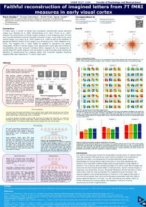
List of Figures 1.1 Comparison of the distribution of pixel values and wavelet coefficients . . . . . . . . . . . . . . . . . . . 1.2 Different stages of undersampling and reconstruction of the sparse signal. . . . . . . . . . . . . . . . . 1.3 Unit spheres ({x : xp = 1}) in R2 induced by different p norms . . . . . . . . . . . . . . . . . . . . . 1.4 Best p norm approximations of x ∈ R2 by a one dimensional subspace D. . . . . . . . . . . . . . . . . 1.5 A broad classification of CS Sparse Reconstruction Algorithms. . . . . . . . . . . . . . . . . . . . . . . . 1.6 The block diagram of Single-pixel Camera. . . . . . . 1.7 SAR image recovery using Notch filtering and sparsity based method. . . . . . . . . . . . . . . . . . . . 1.8 A context diagram of the Thesis contribution. . . . . 2.1 A pictorial demonstration of an underdetermined measurement system, Φ, acting on a signal x0 which has a sparse representation x in an orthonormal basis Ψ. 2.2 A pictorial demonstration of an underdetermined measurement system, A, acting on a K-sparse signal x. . 2.3 A schematic block diagram representing k th iteration of Orthogonal Matching Pursuit (OMP) algorithm. . 2.4 A schematic block diagram representing the k th iteration of Subspace Pursuit (SP) algorithm. . . . . . .

4 6 8 9 10 13 15 18

25 25 37 40

3.1 Schematic block diagram representing the Fusion Framework for Compressed Sensing . . . . . . . . . . . . . 49 3.2 Fusion of two participating algorithms: Gaussian sparse signals . . . . . . . . . . . . . . . . . . . . . . . . . . 63 3.3 Fusion of two participating algorithms: Rademacher sparse signals . . . . . . . . . . . . . . . . . . . . . . 63 xxv

List of Figures 3.4 Fusion of three participating algorithms: Gaussian sparse signal . . . . . . . . . . . . . . . . . . . . . . 64 3.5 Performance of FACS on Real Compressible signals . 66 4.1 Performance comparison of FACS and CoMACS . . . 88 4.2 Performance of the CoMACS and variants for Gaussian Sparse Signals (GSS) and Rademacher Sparse Signals (RSS) . . . . . . . . . . . . . . . . . . . . . . 90 4.3 Performance of CoMACS, 1 based CoMACS (CoMACS_L1) for Gaussian Sparse Signals . . . . . . . . . . . . . . 92 4.4 Performance of CoMACS, L1 based CoMACS (CoMACS_L1) for large dimensional problems . . . . . . 94 4.5 Performance of CoMACS based methods for ECG signals . . . . . . . . . . . . . . . . . . . . . . . . . . . 95 5.1 Progressive performance of pFACS for Rademacher sparse signals . . . . . . . . . . . . . . . . . . . . . . 108 5.2 Performance of pFACS for real-world ECG signals . . 111 6.1 Performance of MMV-FACS for Gaussian sparse signal matrices, varying the number of measurements (M) . . . . . . . . . . . . . . . . . . . . . . . . . . . 6.2 Performance of MMV-FACS for Rademacher sparse signal matrices, varying the number of measurements (M) . . . . . . . . . . . . . . . . . . . . . . . . . . . 6.3 Performance of MMV-FACS for Gaussian sparse signal matrices, varying the number of measurement vectors (L) . . . . . . . . . . . . . . . . . . . . . . . 6.4 Performance of MMV-FACS for Gaussian sparse signal matrices, varying SMNR . . . . . . . . . . . . . . 6.5 Performance of MMV-FACS for real compressible signals . . . . . . . . . . . . . . . . . . . . . . . . . . . 7.1 Progression of IFSRA(MP) over iterations for Gaussian sparse signal . . . . . . . . . . . . . . . . . . . . 7.2 Performance of IFSRA(MP) under measurement perturbations . . . . . . . . . . . . . . . . . . . . . . . . 7.3 Performance of IFSRA(CoSaMP) under measurement perturbations . . . . . . . . . . . . . . . . . . . . . . 7.4 Performance of IFSRA(BPDN) under measurement perturbations . . . . . . . . . . . . . . . . . . . . . . xxvi

136

137

138 139 140 153 167 167 168

List of Figures 7.5 Performance comparison of IFSRA(MP), IFSRA(CoSaMP), and IFSRA(BPDN) under measurement perturbations 169 7.6 Performance of IFSRA for ECG signals from MIT-BIH Arrhythmia Database . . . . . . . . . . . . . . . . . . 170

xxvii

List of Tables 3.1 Average number of correctly estimated atoms by OMP and SP, for GSS, in clean measurement case . . . . . 46 3.2 Performance of FACS on a highly coherent dictionary matrix: . . . . . . . . . . . . . . . . . . . . . . . . . . 67 4.1 Ratio of average number of true atoms in common support-set and average cardinality of common supportset, for GSS, in clean measurement case . . . . . . . 75 5.1 Comparison of average computation time (in seconds) by different fusion algorithms for Rademacher sparse signals (RSS) . . . . . . . . . . . . . . . . . . 110

xxix

To my grandparents

xxxi

CHAPTER

1

Introduction “The last thing that we find in making a book is to know what we must put first.” Blaise Pascal [1623-1662]

Signal processing community has been interested in sparse signal reconstruction for a long time. The vast activity in the years 1980 − 2000 on transforms and transform coding, particularly in wavelets and frame theory, significantly contributed to this field. The highly influential works in the mid-nineties [1–3] brought out the importance of treating sparse signal reconstruction as an individual research area. Inspired by this, a lot of extensive works on sparse signal modelling took place in the past decade. Donoho and Huo [4] established a theoretical connection, for the first time, between the sparsity seeking transforms and the 1 -norm measure. The seminal works by Donoho [5,6] and Candès et al. [7–9] ignited a burst of interest in sparse signal modelling by mathematicians (theorists and applied), statisticians, physicists, geophysicists, neuropsychologists, engineers from various fields, computer science theoreticians, and others. A large number of conferences, workshops, and special sessions have been organized in these topics in 1

Chapter 1

Introduction

recent years. Prestigious journals in the field have allocated special issues for sparse signal modelling and related topics. For example, IEEE-SPL EDICS recently added many entries related to sparse signal modelling. All of these are testimonials for the great attention received by this field. In this thesis, we deal with a special class of sparse signal modelling problems called Compressed Sensing (CS), which has received wide attention after the pioneering works of Donoho [5, 6] and Candès et al. [7–9]. CS combines sampling and compression of the signal of interest through a non-adaptive, under-sampled linear measurement setup. Though CS was introduced only in the last decade, it has been manifested as a revolution and still one of the most intensively researched topic in many areas like signal processing, sensor systems, and machine learning. Next, we briefly discuss an application where CS has already made life-altering impacts. One of the key advantages of CS is that it offloads the complexity from data acquisition to data reconstruction. In many applications, the data acquisition is critical as the acquisition time and other resources, including hardware, are very limited. For example, CS has already made life-altering impacts in Magnetic Resonance Imaging (MRI) , which is an essential tool of modern medical imaging. MRI plays a key role in investigating the anatomy and function of the body in both health and disease. High resolution MRI requires the patient to lie very still, even the heartbeat need to be stopped, during the measurement process and the imaging speed is often critical for the life of the patient in many MRI applications. Also, in many situations a slow MRI scan may not be feasible due to other reasons [10]. Hence, any significant speed improvement in MRI data acquisition will be life altering. However, the physical (gradient amplitude and slew-rate) and physiological (nerve stimulation) constraints fundamentally limit the speed of MRI data 2

Chapter 1

Introduction

acquisition [11]. It has been shown that, by exploiting the transform sparsity inherent in MR images, the data acquisition can be sped up by a factor of 7 [12] using the principles of CS.

1.1 Compressed Sensing and Sparse Signal Processing In CS setup, we assume that the signal-of-interest is sparse/compressible in some orthonormal basis and the task is to recover the signal from under-sampled measurements by exploiting the sparse/compressible nature of the signal. That is, in CS the signal x0 ∈ RN ×1 is modelled as a superposition of a few columns of a given matrix Ψ ∈ RN ×N . In other words, we have, x0 = Ψx where x is sparse. Consider a linear measurement setup b = Ax where A ∈ RM ×N represents the measurement system. For example, in MRI applications, A may be formed from a few rows of the DFT matrix and Ψ may be chosen as a wavelet basis matrix. In this thesis, we assume that Ψ is an identity matrix so that x itself is sparse. In CS, the strive is to reduce the number of measurements, M, without compromising on the reconstruction quality. In this thesis, we focus on the methods to improve the estimate of the sparse signal given A and b.

1.1.1

How Good is the Sparse Assumption?

In practice, we rarely meet exactly sparse signals. However, many signals we deal in applications are found to be sparse or compressible in some transform domain. For example, many images, especially natural images, are highly compressible in the wavelet domain. To elaborate more on this claim, consider the image shown 3

Chapter 1

Introduction

in Figure 1.1(a). This is an aerial view of the main building of Indian Institute of Science (IISc).

(a) Image: IISc main buiding (size: 456 x 636 x 3)

(b) Single-level 2D-Wavelet Decompostition (four subimages each having size 228 x 318 x 3)

0.08 0.5 Normalized Histogram

Normalized Histogram

0.07 0.06 0.05 0.04 0.03 0.02

0.3 0.2 0.1

0.01 0 0

0.4

100 200 Pixel Values

0 0

255

(c) Histogram of pixel values of the original image

100 200 Wavelet Coefficients

255

(d) Histogram of the wavelet coefficients

F IGURE 1.1: Comparison of the distribution of pixel values in an image and the coefficients of its single-level two-dimensional wavelet decomposition (Figure 1.1(a) courtesy:       ).

The single-level two-dimensional wavelet decomposition with respect to the Haar wavelet [13] of Figure 1.1(a) is shown in Figure 1.1(b). The wavelet decomposition was done independently on the three colour panes (red, green, and blue) of the original image. The upper left sub-image in Figure 1.1(b) shows the image reconstructed from the approximation coefficient matrix and the 4

Chapter 1

Introduction

other three sub-images are reconstructed from the details coefficients matrices of the single-level two-dimensional wavelet decomposition. The normalized histogram of the pixel values of the image shown in Figure 1.1(a) is given in Figure 1.1(c). Figure 1.1(d) shows the normalized histogram of the coefficients of the single-level twodimensional wavelet decomposition of the original image. It may be observed from Figure 1.1(c) and Figure 1.1(d) that the wavelet representation of this image is approximately sparse. That is, most of the wavelet coefficients of the image are close to zero. Sparsity is one of the key assumptions in CS and this is an example to show that sparse signals are ubiquitous in practice.

1.2 Sparse Reconstruction Algorithms In a CS setup, the number of measurements available may be significantly smaller than the dimension of the sparse signal. The reconstruction requires to solve a highly underdetermined system of equations which will result in an infinite number of solutions, in general [14]. However, using CS theory, it has been shown that robust signal reconstruction is possible by exploiting sparse nature of the signal [6–8, 15]. According to the celebrated Whittaker-Nyquist-KotelnikovShannon theorem [16–19], a signal can be reconstructed if the sampling rate is at least twice its bandwidth. If this criterion is not satisfied, aliasing occurs, and in general it is not possible to discern an unambiguous signal. To develop an intuition for reconstructing the signals from the undersampled data, consider the scenario presented in Figure 1.2 [20]. 5

Chapter 1

Introduction

F IGURE 1.2: Different stages of undersampling and reconstruction of the sparse signal. (a) Frequency spectrum of a sparse signal with 3 nonzero components (b) Signal in time-domain with two sampling criteria: uniform undersampling (lower red bubbles) and random undersampling (upper red dots) (c) Interference occurs due to random undersampling but the two strong components are above the interference level (d) Severe interference due to uniform undersampling makes signal reconstruction impossible (e) Thresholding (f) Reconstruction of the two strong components (h) The interference caused by the two strong components estimated (g) Subtraction and thresholding recovers the weak component (figure courtesy: [20]).

In this figure, we consider a signal which is sparse in the frequency domain. Figure 1.2(a) shows the frequency spectrum of a sparse signal with 3 non-zero elements. We use two sampling criteria: uniform undersampling (lower red bubbles) and random undersampling (upper red bubbles) to sample the signal as shown in Figure 1.2(b). The results of random under sampling and uniform undersampling are depicted in Figure 1.2(c) and Figure 1.2(d) respectively. It may be observed from Figure 1.2(d) that the uniform undersampling resulted in severe aliasing preventing signal reconstruction. However, though aliasing also occurs in the case of random undersampling as shown in Figure 1.2(c), the two strong signal components appear well above the interference level caused by aliasing. These two strong signal components are detected and identified using thresholding as shown in Figure 1.2(e) and Figure 1.2(f). The interference due to the two signal components are calculated and shown in Figure 1.2(h). This estimated interference 6

Chapter 1

Introduction

is subtracted from the aliased signal to get the signal shown in Figure 1.2(g). Another thresholding on the signal on Figure 1.2(g) recovers the remaining (weak) component of the sparse signal. Figure 1.2 shows that a random sampling strategy preserves the information of a sparse signal even in an undersampled data and using efficient reconstruction algorithms perfect (near-perfect) signal reconstruction is possible.

1.2.1

p Norm: Building the Intuition for Sparse Signal Reconstruction

In this section, we briefly discuss the role of p norm (p ∈ [0, ∞]) in CS which will help to build an intuition behind the principles of Sparse Reconstruction Algorithms (SRAs). ˆ denote an estimate of the signal x. Generally we use Let x p norm to measure the approximation error. For a signal x = [x1, x2, . . . , xN ]T , p norm is defined as ⎧ ⎪ ⎪ | (x)| , ⎪ ⎪ ⎪  p1 ⎪ N ⎨ p xp = |xi| , ⎪ ⎪ i=1 ⎪ ⎪ ⎪ ⎪ ⎩ max |xi |, i=1:N

p = 0; p ∈ (0, ∞);

(1.1)

p = ∞.

Note that p -norm satisfies all the properties of norm iff p ≥ 1. For p ∈ (0, 1), p norm is only a quasi-norm. The 0 norm is not even a quasi-norm. However, we can show that lim xpp = | (x)| = p→0

x0, which justifies the choice of the notation used. Different p norms have different properties as illustrated in Figure 1.3, and as 7

Chapter 1

Introduction

we describe next, the choice of p -norm plays a major role in sparse reconstruction problems.

(a) 1 -norm

(b) 2 -norm

(c) ∞ -norm

(d)  1 -norm 2

F IGURE 1.3: Unit spheres ({x : xp = 1}) in R2 induced by different p norms (p = 1, 2, ∞, 21 ) (figure courtesy: [21]) .

To illustrate the role of different p norms in sparse signal reconstruction, consider a sparse signal x ∈ R2 which has only one non-zero element. Consider the problem of finding an approximation for x, using a point in a one-dimensional affine space D. ˆ ∈ D which In p norm sense, this can be achieved by finding x ˆ p . Finding the closest approximation of x in D minimizes x − x using p norm may be viewed as growing an p sphere (more precisely, a circle in the R2 case) centered on x until it touches D. The intersecting point will be the closest point to x in the chosen p norm sense. This scenario for different p norms are illustrated in Figure 1.4. We may observe that p -norm intersects with D at different values for p = 1, 2, ∞. It may be observed from Figure 1.4 that the evenness of the distribution of error among the two coefficients are directly proportional to p. That is, a smaller p promotes sparsity. For example 1-norm intersects with D on the axis where 8

Chapter 1

Introduction

ˆ will be sparse as x is sparse. However, as it may x lies. Hence x be observed from Figure 1.4, 2 -norm and ∞ norm will not yield a sparse solution. A generalization of this behaviour may also be observed in higher dimensional problems and it plays an important role in sparse signal reconstruction problems. ˆ1 x

ˆ2 x D

x

(a) 1 -norm

(b) 2 -norm

ˆ1 x 2

ˆ∞ x D

x

D

x

D

x

(c) ∞ -norm

(d)  1 -norm 2

F IGURE 1.4: An illustration of the best p norm approximations, for p = 0, 1, 2, ∞, 12 , of x ∈ R2 by a one dimensional subspace D (figure courtesy: [21]).

For CS signal reconstruction, the optimal method is solving an 0 -minimization problem, which is Non-deterministic Polynomialtime hard (NP-hard). For practical implementations, many suboptimal algorithms are introduced in recent years which may be broadly categorized into four classes as shown in Figure 1.5.

9

Chapter 1

Introduction LASSO [37]

BPDN [36]

ISD [35]

DS [38]

LARS [39]

BP [2]

Convex Relaxation Methods

SBL [34]

Non Convex Minimization Methods

IRL1 [33]

FOCUSS [32]

CS Sparse

Modified BPDN [40]

Reconstruction

StOMP [31]

Algorithms FSA [22]

IHT [30]

Combinatorial Methods CP [23]

Greedy Pursuits CoSaMP [29]

MP [1]

HHS [24]

OMP [26, 27]

Sudocodes [25]

SP [28]

F IGURE 1.5: A broad classification of CS Sparse Reconstruction Algorithms.

Next, we briefly discuss each category. A more elaborated discussion on a few SRAs, relevant for the thesis, is given in Chapter 2.

1.2.2

Convex Relaxation Methods

Convex relaxation methods are so popular in CS literature that many consider it as a synonym for SRAs. This is mainly due to the fact that Convex Relaxation Methods (CRM) were the first to 10

Chapter 1

Introduction

provide elegant theoretical guarantees for sparse signal reconstruction in the CS framework. Another factor is the off-the-shelf availability of excellent toolboxes to solve convex problems efficiently and accurately. In convex relaxation methods, the 0 minimization problem is relaxed using an 1 minimization problem. Examples of popular CRM include Basis Pursuit (BP) [2] and Basis Pursuit De-Noising (BPDN) [36], modified BPDN [40], Least Absolute Shrinkage and Selection Operator (LASSO) [37,41], Least Angle Regression (LARS) [39], and Dantzig Selector (DS) [38]. The number of measurements required by CRM for exact signal reconstruction is small. However, CRM are computationally very expensive which make them less attractive for practical applications.

1.2.3

Greedy Pursuits

Greedy pursuits find the estimate of the sparse signal step by step, in an iterative fashion. They possess simple geometric interpretations and like CRM, many of them show elegant theoretical guarantees. The advantages in terms of computational complexity and memory requirements make them more attractive for applications. The popular greedy pursuits include Matching Pursuit (MP) [1], Orthogonal Matching Pursuit (OMP) [26, 27], Stage-wise Orthogonal Matching Pursuit (StOMP) [31], Subspace Pursuit (SP) [28], Compressive Sampling Matching Pursuit (CoSaMP) [29], and Iterative Hard Thresholding (IHT) [30].

11

Chapter 1

1.2.4

Introduction

Combinatorial Algorithms

Greedy pursuits provide computational advantage over CRM, both empirically and theoretically. Combinatorial methods are significantly fast and efficient than both CRM and greedy pursuits. However, these methods require specific pattern in the measurements which may not be feasible to realize in many applications. They reconstruct sparse signals following the principles of group testing [42]. The popular algorithms in this area include Heavy Hitters on Steroids (HHS) [24], Chaining Pursuits (CP) [23], Fourier Sampling Algorithm (FSA) [22], and Sudocodes [25].

1.2.5

Non Convex Minimization Algorithms

It has been shown that, instead of relaxing 0 minimization problem to an 1 minimization problem, we may also solve non convex relaxation problems for efficient sparse signal reconstruction. A popular method is to replace 0 minimization with q minimization problem where 0 < q < 1. Another strategy is to use a Bayesian framework which exploits the sparse nature of the signal. Examples of the popular work in this family are Iterative Re-weighted L1 (IRL1) [33], Iterative Support Detection (ISD) [35], and Sparse Bayesian Learning (SBL) [34, 43–46].

1.3 Applications of CS In many applications it is highly desirable to reduce the number of measurements without reducing the reconstruction quality since it gives several advantages like reduction in the number of sensors, simpler hardware design, faster acquisition time, and less power 12

Chapter 1

Introduction

consumption. Due to these potential advantages, though CS is a relatively new area, it has been successfully applied in many fields. In this section, we briefly discuss some of the applications.

1.3.1

Compressive Imaging

CS has far reaching implications in imaging as it reduces the number of measurements and hence cut down power consumption, storage space, hardware complexity, and acquisition time. The single pixel camera [47] developed by Rice university is one of the first applications built using CS principles. The block diagram of single pixel camera is given in Figure 1.6. Recently Huang et al. [48] proposed a lensless compressive imaging architecture for capturing images of visible and other spectra such as infrared, or millimeter waves.

F IGURE 1.6: The block diagram of Single-pixel Camera. (source:         )

CS has also found life altering applications in the field of medical imaging. It has been used to reduce the MRI scanning time [11, 20]. CS has also been successfully applied to seismic imaging [49].

13

Chapter 1

1.3.2

Introduction

Compressive RADAR/SONAR

Radio Detection and Ranging (RADAR) and Sound Navigation and Ranging (SONAR) are widely used in many civilian, military, and bio-medical applications. However, the resolution in these applications are limited by the classic time-frequency uncertainty principles. CS has been shown to produce promising results in images of RADAR/SONAR using relatively a smaller number of measurements than the conventional methods. Compressive RADAR eliminated the need of pulse compression matched filter at receiver and reduces A/D conversion bandwidth which simplifies the hardware design [50]. Sparse sampling has been applied to both time and frequency domain to enhance pulse compression technique in order to efficiently compress, restore and recover the RADAR data [51–53]. The optimization of waveforms for CS application in RADAR is discussed by He et al. [54] and Kyriakides et al. [55]. CS has also found applications in Passive coherent location (PCL) [56, 57], Synthetic Aperture RADAR (SAR) [58–60], through-the-wall RADAR [61], and SONAR and ground penetrating RADAR [62–64]. The advantage of using CS in SAR image recovery is shown in Figure 1.7. CS has also been widely used in many other applications like Compressive micorarrays [65], group testing [66], A/D converters [67,68], communication and networks. Examples include sparse channel estimation [69,70], spectrum sensing [71,72], ultra wideband systems [73], wireless sensor networks [74], network management [75], network data mining [76] and network security [77]. A more elaborated list of applications and references can be found at [78] and [79].

14

Chapter 1

Introduction

F IGURE 1.7: SAR image recovery of close targets using Notch filtering and sparsity based method.

1.4 Challenges/ Problems Identified Though many SRAs possess elegant theoretical guarantees for sparse signal recovery, it is well known that the performance of any sparse recovery algorithm depends on several factors like signal dimension, sparsity level of signal, and measurement noise power [8,80– 82]. Empirically, it has been also observed that the recovery performance varies significantly and depends on the underlying statistical distribution of the non-zero elements of the sparse signal [81, 82]. If this distribution is known a priori, we can employ the best recovery algorithm suitable for that type of signal and get the best sparse signal estimate. In many practical applications, we may not have this prior knowledge and hence, we cannot use the appropriate method to achieve the best performance. It can be also seen that every sparse recovery algorithm requires a minimum number of measurements (algorithm dependent) for sparse signal recovery and performs poorly in a very low dimension measurement scenario [81–84]. The reduction in number of measurements leads to reduction in the number of sensors and/or 15

Chapter 1

Introduction

reduction in the measurements time. Hence in many applications, it is highly desirable to have a reduced number of measurements. For example, in IR camera [85], the sensors are very costly. In medical applications like MRI, where we have to even stop the heartbeat of the patient during the measurements process to get a high resolution MRI, the reduction in measurement time is often critical for the life of the patient [11]. Though it is evident that the performance of the sparse recovery algorithms degrades in cases where only a limited number of measurements are available or the statistical distribution of the sparse signal is unknown, it is interesting to observe (empirically) that this degradation does not always imply a complete failure [81,82]. The estimate obtained by the algorithm will often contain partially correct information about the sparse signal. By exploiting the partial information about the target signal, it may be possible to get a better sparse signal estimate. In this thesis, we explore this possibility and propose novel methods to improve the performance of arbitrary sparse signal reconstruction algorithms.

1.5 Contributions In this thesis, we propose novel frameworks and algorithms to improve the performance of any arbitrary SRA. • We propose a fusion framework which fuses the estimates of multiple participating algorithms to result in a better sparse signal estimate. • We also propose an iterative framework which improves the performance of any arbitrary sparse signal reconstruction algorithm without modifying the underlying algorithm. 16

Chapter 1

Introduction

Fusion Framework To improve the sparse signal estimate, we propose a fusion framework where we employ multiple SRAs which are run in parallel, independently. The estimates obtained by these participating algorithms are fused efficiently to get a sparse signal estimate which is often better than the best estimate provided by the participating algorithms independently. We propose different schemes for fusion. The proposed schemes use the participating algorithm as a black box, and does not require any change in the underlying participating algorithm. We mathematically analyse the proposed schemes and verify the robustness against signal and measurement perturbations. We demonstrate the efficiency and effectiveness of the proposed methods in applications through extensive numerical experiments on both synthetic and real-world data.

Iterative Framework: In the iterative framework, we exploit the partial information about the sparse signal available in the estimate obtained by a given arbitrary SRA. We use this information in the subsequent iterations to improve the sparse signal reconstruction iteratively. The proposed iterative algorithm is also general in nature, which can incorporate any SRA as a participating algorithm. We derive convergence guarantees for the proposed algorithm, and demonstrate its advantage in applications using simulations.

17

Chapter 1

Introduction

A context diagram of the Thesis contribution is shown in Figure 1.8.

Reduced Number of Measurements [88, 89]

Optimize Projection Matrix [86, 87]

Projection Matrix Theory

Compressed Sensing Theory

Reconstruction Algorithms

Convex Relaxation [2, 36, 37, 39]

Greedy Pursuits [27–29, 90]

Non-Convex Methods [32–35]

Combinatorial Algorithms [22–25]

Sparse Signal Estimate

Sparse Signal Estimate

Sparse Signal Estimate

Sparse Signal Estimate

Contribution of the Thesis Improved Sparse Signal Estimate!

F IGURE 1.8: A context diagram of the Thesis contribution.

1.6 Organization of the Thesis In this section, we give an overview of the organization of the thesis and briefly discuss the contributions in each chapter. 18

Chapter 1

Introduction

Chapter 2 In Chapter 2, we briefly introduce CS and discuss a few desirable properties of the measurement system which are sufficient to guarantee signal reconstruction. We also illustrate a few popular SRAs widely used in subsequent chapters of this thesis. We also provide some existing theoretical results which will be useful while theoretically analysing the proposed methods.

Chapter 3 In Chapter 3, we explain the motivation behind this research and develop a framework to fuse the estimates of multiple participating algorithms. We also propose a fusion algorithm called Fusion of Algorithms for Compressed Sensing (FACS) and derive theoretical guarantees for performance improvement. Then we perform extensive numerical experiments using some of the well known SRAs in CS which confirms the effectiveness of the proposed scheme. The work described in this chapter has been published in IEEE Transactions of Signal Processing [91].

Chapter 4 We propose another fusion algorithm called Committee Machine Approach for Compressed Sensing (CoMACS) in Chapter 4. Variants of CoMACS are also proposed here to further enhance the sparse reconstruction quality. We also study the theoretical aspects of the proposed methods. We also show that the proposed algorithms produce better sparse signal estimates compared to the participating algorithms. The work summarized in this chapter has been published in IEEE Transactions on Signal Processing [92]. 19

Chapter 1

Introduction

Chapter 5 FACS and CoMACS are not latency friendly algorithms. For low latency applications, we propose a latency friendly fusion algorithm called progressive Fusion of Algorithms for Compressed Sensing (pFACS) in Chapter 5. We also discuss the theoretical guarantees of pFACS and show the efficacy of pFACS using extensive numerical experiments. This work has been published in Signal Processing [93].

Chapter 6 In Chapter 6, we extend the fusion framework and FACS to the Multiple Measurement Vector (MMV) problem. We theoretically analyse the proposed algorithm and derive sufficient conditions for improving the performance. Further, we corroborate the claim with the average case analysis. Using extensive simulations, we show that the proposed method provides significant performance improvement.

Chapter 7 In Chapter 7, we develop a novel iterative framework called Iterative Framework for Sparse Reconstruction Algorithms (IFSRA) which can be used to improve the performance of any arbitrary SRA. We theoretically analyse IFSRA and derive convergence guarantees. Using numerical experiments, we show that IFSRA improves performance of SRAs. This work that has been published in Signal Processing [94].

20

Chapter 1

Introduction

Chapter 8 In Chapter 8, we give the conclusions we have drawn from our research and suggest a few ideas for related future work.

1.7 Summary In this chapter, we briefly discussed the importance of sparse signal modelling, sparse signal processing and CS. The we discussed a few applications to motivate about the significance of compressed sensing and sparse signal processing. We also used a few examples to give the intuition behind the working principles of CS and sparse signal reconstruction. A few challenges identified in this field and the solutions offered in this thesis are also briefly discussed in the later part of this chapter.

21

CHAPTER

2

CS and Sparse Signal Reconstruction: Background “I may not agree with what you say, but I’ll defend to the death your right to say it.” Voltaire [1694-1778]

First, we briefly review Compressed Sensing (CS). Then we discuss some theoretical results and a few popular Sparse Reconstruction Algorithms (SRAs) in CS which are widely used in the subsequent chapters.

2.1 Signal Models With the seminal works of Donoho [5] and Candès et al. [8, 15], CS has emerged as a new framework for signal acquisition which allows large reduction in the cost of acquiring signals that have a sparse or compressible representation in some transform domain. Consider a standard measurement system that produces M linear 23

Chapter 2

CS and Sparse Signal Reconstruction: Background

measurements of the signal x0 ∈ RN ×1 which can be mathematically expressed as b = Φx0 + w,

(2.1)

where Φ ∈ RM ×N represents the measurement system, b ∈ RM ×1 represents the measurement vector, and w ∈ RM ×1 represents the additive measurement noise present in the system. Let the signal x0 have a K-sparse representation in some transform domain with orthonormal basis Ψ ∈ RN ×N . Let x ∈ RN ×1 denote the K-sparse representation of x0 such that x0 = Ψx.

(2.2)

Note that, x is a K-sparse signal. Mathematically, a signal is said to be K-sparse, if it has at most K non-zero elements (x0 ≤ K). Let T denote the support-set1 of x with |T | ≤ K. Combining (2.1) and (2.2), we get b = ΦΨx + w.

(2.3)

A pictorial representation of (2.3) is given in Figure 2.1. We can re-write (2.3) as b = Ax + w, where A = ΦΨ ∈ RM ×N . Unless otherwise stated, throughout this thesis, we assume Ψ = I so that A represents the measurement system. That is, in this thesis, we consider the standard CS measurement setup which acquires a K-sparse signal x ∈ RN ×1 using 1

Support-set of a vector is defined as the set of indices of non-zero elements of the vector.

24

Chapter 2

bM×1

CS and Sparse Signal Reconstruction: Background

ΦM×N

ΨN×N

xN×1 wM×1

=

+

K-sparse



 x0



F IGURE 2.1: A pictorial demonstration of an underdetermined measurement system, Φ, acting on a signal x0 which is has a sparse representation x in an orthonormal basis Ψ (original source: [95]).

M( N ) linear measurements via the following relation b = Ax + w,

(2.4)

where b ∈ RM ×1 denotes the measurement vector, A ∈ RM ×N denotes the measurement matrix, and w ∈ RM ×1 denote the additive measurement noise. The measurement matrix A is also called projection matrix in literature. A pictorial representation of (2.4) is shown in Figure 2.2.

bM×1

AM×N

=

xN×1

wM×1

+

K-sparse

F IGURE 2.2: A pictorial demonstration of an underdetermined measurement system, A, acting on a K-sparse signal x (original source: [95]).

25

Chapter 2

CS and Sparse Signal Reconstruction: Background

Note that (2.4) is an underdetermined system and solving x from (2.4) is an ill-posed problem, in general [14]. In the noiseless case (w = 0), (2.4) may be also viewed as dimensionality reduction of a high dimensional sparse vector. There are two main theoretical questions in CS : i) How should we design the measurement matrix A to ensure that it preserves the information in the signal x? ii) How can we reconstruct the original signal x from the measurements b?

2.2 Measurement System The measurement matrix A in (2.4) may be viewed as a dimensionality reduction operator which maps signals in RN ×1 to RM ×1 (M  N ). CS strives to reduce the measurements without compromising on the reconstruction quality. Hence, efficient design of the measurement system A involves two main tasks: i) To reduce the number of measurements as far as possible, ii) To preserve the information of the signal in the measurements. A few desirable properties for efficient designs of A are discussed below.

2.2.1

Null Space Property (NSP)

Let ΣK = {x ∈ RN ×1 : x0 ≤ K} denote the set of all K-sparse signals in the N -dimensional space. Let N (A) = {z : Az = 0} 26

Chapter 2

CS and Sparse Signal Reconstruction: Background

denote the null space of A. To recover all K-sparse signals from the measurements b, it is necessary and sufficient that, for any pair of distinct K-sparse vectors x1 and x2 , we must have, Ax1 = Ax2. Formally, A uniquely represents all x ∈ ΣK iff N (A) does not contain any 2K sparse vectors. This property is widely characterized by spark [96] which is defined as follows. Definition 2.1 (Spark [96]). Spark of matrix A is defined as the smallest number of linearly dependent columns of A. Theorem 2.1 (Corrollary 1 of [96]). For any vector b ∈ RM ×1, there exists at most one signal x ∈ ΣK such that b = Ax if and only if spark(A) > 2K. For A ∈ RM ×N (2 ≤ M < N ), we have, 2 ≤ spark(A) ≤ M + 1. Hence, as a consequence of Theorem 2.1, we have M ≥ 2K is a necessary condition for unique sparse signal recovery. Though for exact K-sparse signals spark provides a necessary and sufficient condition for sparse signal recovery, for approximately sparse signals (compressible signals) more restrictive conditions on null space, called Null Space Property (NSP) [97], is required. Definition 2.2. A matrix A satisfies the NSP of order K if there exist a C > 0 such that



zT c zT1 2 ≤ C √ 1 1 K holds for all z ∈ N (A) and for all T1 ⊂ {1, 2, 3, . . . , N } with |T1 | ≤ K. While NSP provides a necessary and sufficient condition for establishing convergent guarantees (typically upper bounds on reconstruction errors) for arbitrary signals, these guarantees do not 27

Chapter 2

CS and Sparse Signal Reconstruction: Background

cater for errors due to measurement noise or quantization. Candès et al. [7–9] introduced an isometric condition on the measurement matrix called Restricted Isometry Property (RIP). In this thesis, we extensively use RIP while theoretically analysing our proposed methods.

2.2.2

Restricted Isometry Property (RIP)

Definition 2.3. A matrix A satisfies RIP [7–9] if there exist a constant δ ∈ [0, 1) such that (1 − δ) x22 ≤ Ax22 ≤ (1 + δ) x22

(2.5)

holds for any K-sparse vector x. The Restricted Isometry Constant (RIC) δK ∈ [0, 1) is defined as the smallest constant for which RIP property holds for all K-sparse vectors. If A satisfies RIP of order 2K, then A approximately preserves the distance between any pair of K-sparse vectors. RIP may be viewed as a less general form of stable embedding property [98] of sparse vectors. Next we discuss a few results due to RIP, which will be widely used in the theoretical discussions of subsequent chapters of this thesis. Proposition 2.1. (Proposition 3.1 in [29]) Let A have RIC δr and let T denote a set of r indices or fewer. Then, for an arbitrary z, we have

 −1 1

H

z ≤ z2 ,

AT AT 2 1 − δr

1

z2 . and A†T z ≤ √ 2 1 − δr 28

(2.6) (2.7)

Chapter 2

CS and Sparse Signal Reconstruction: Background

Proposition 2.2. (Proposition 3.2 in [29]) Let A have RIC δr . Let T1 and T2 be two disjoint sets of indices of columns of A such that |T1 ∪ T2 | ≤ r. Then AH (2.8) T1 AT2 2 ≤ δr . Corollary 2.1. (Corollary 3.3 in [29]) Let A have RIC δr and let S denote a set of column indices from A. Let x be a sparse vector with support-set T such that r ≥ |T ∪ S|. Then we have AH S AS c xS c 2 ≤ δr xS c 2 .

(2.9)

Proposition 2.3. (Lemma 2 in [28]) Consider A ∈ RM ×N , and let T1 , T2 be two subsets of {1, 2, . . . , N } such that T1 ∩ T2 = ∅. Assume that δ|T1 |+|T2 | < 1, and let y ∈ span(AT1 ) and r = y − AT2 A†T2 y, then we have   δ|T1 |+|T2 | y2 ≤ r ≤ y2. (2.10) 1− 1 − δmax (|T1 |,|T2 |) Lemma 2.1. (Lemma 3 in [28]) Consider the measurement system b = Ax + w, where x ∈ RN is a K-sparse signal vector, w ∈ RM denote the additive measurement noise, and A ∈ RM ×N represent the sampling matrix with RIC δK . For an arbitrary set ˆ T1 = A†T1 b and x ˆ T1c = 0. T1 ⊂ {1, 2, . . . , N } with |T1 | ≤ K, define x Then, the following inequality holds. ˆ 2 ≤ x − x

1 1 + δ2K

w2 .

xTˆ1c + 2 1 − δ2K 1 − δ2K

Note that though the result in Lemma 3 of [28] contains only δ3K , the lemma is even valid for δ2K (see proof of Lemma 3 in [28] for more details).

29

Chapter 2

CS and Sparse Signal Reconstruction: Background

Lemma 2.2. (Lemma 15 in [24]) Let the measurement matrix A ∈ RM ×N have RIC δK . Then for an arbitrary x ∈ RN ×1, we have Ax2 ≤

   1 1 + δK x2 + √ x1 . K

2.2.2.1 Measurement bounds using RIP The following theorem gives a lower bound on the number of measurements (M) to achieve RIP. Theorem 2.2 (Theorem 3.5 of [99]). Let A ∈ RM ×N satisfies RIP of order 2K with RIC δ2K ∈ (0, 12 ]. Then M ≥ CK log(

N ), K

(2.11)

√ where C = 12 log( 24 + 1) ≈ 0.28.

2.2.3

Coherence

Though spark, NSP, and RIP provide theoretical guarantees for the recovery of sparse signals, verifying whether a given matrix satisfies these properties is a highly combinatorial problem which requires   extensive search over all N K sub-matrices. Unlike these properties, coherence [27, 96] of a matrix is easily computable which can also provide convergence guarantees for the recovery of sparse signals. Definition 2.4 (Coherence). The coherence of a matrix A ∈ RM ×N , denoted by μ(A), is defined as the largest absolute inner product between any pair of columns ai and aj (i = j) of A: μ(A) = max

1≤i
30

|ai , aj | ai 2aj 2

Chapter 2

CS and Sparse Signal Reconstruction: Background

 We have, for any matrix A ∈ RM ×N , MN(N−M −1) ≤ μ(A) ≤ 1. The lower bound is known as the Welch bound [100–102] which can be approximated by √1M for M  N . Under certain conditions coherence can be related to the spark, NSP, and RIP. For example, 1 . spark(A) ≥ 1 + μ(A)

2.2.4

Measurement Matrix Constructions

Though many schemes have been proposed to construct measurement matrix, the most optimal construction in terms of the number of measurements is provided by the random matrix constructions. It has been also shown that the random matrices will satisfy the RIP with high probability if the entries are chosen from a sub-Gaussian distribution [5, 15]. The linkage between the RIP property of random matrices and Johnson-Lindenstrauss (JL) lemma [103] was studied by Baraniuk et al. [104] and derived a simpler proof of the RIP for random matrices. The measurements obtained using random matrices are democratic, which in general contains equal information about the measured signal. Hence random measurement matrices are robust to the measurement noise up to a reasonable level. Examples of sub-Gaussian distributions include Gaussian and Bernoulli distributions. In this thesis, we use Gaussian random matrices as the measurement matrices in the numerical experiments. In practice, we may be interested in acquiring a signal which is sparse w.r.t. some orthonormal basis Φ. If A is a Gaussian random matrix, similar to A, AΦ will also satisfy RIP with high probability for sufficiently large M [104].

31

Chapter 2

CS and Sparse Signal Reconstruction: Background

2.3 Reconstruction Algorithms Let us assume that our measurements are noise-free such that (2.4) reduces to b = Ax.

(2.12)

Reconstructing x from a small number of measurements from (2.12) is an ill-posed problem and unique signal reconstruction is not possible, in general. However, for a K-sparse signal, unique signal reconstruction is possible by solving an optimization problem of the form min x0

subject to

Ax = b,

(2.13)

provided spark(A) > 2K. We rarely meet exactly sparse signals in practice. However, many signals found in real life are compressible or compressible in some transform domain. Also, in many applications, we need to cater for the noise present in the measurement system. In such situations, we rather solve a robust version of (2.13), given as min x0

subject to

x

Ax − b2 ≤ ,

(2.14)

where  represents the tolerance factor for signal and measurement contamination. It is interesting to note that (2.14) may be expressed in two alternate, but equivalent ways. An unconstrained alternative for (2.14) is given by min x0 + λAx − b2, x

32

(2.15)

Chapter 2

CS and Sparse Signal Reconstruction: Background

where λ represents a regularization parameter which controls the trade-off between the sparsity of the solution and its fidelity with the measurements. Another equivalent alternative can be written as min Ax − b2 x

subject to x0 ≤ K,

(2.16)

where we specify the desired level of sparsity, K. Solving these optimization problems require an extensive search through all possible sets of K columns of A. Unfortunately, this is a Non-deterministic Polynomial-time hard (NP-hard) problem [105]   which leaves N K possibilities. Hence this strategy is not feasible even for the modest values of N and K. Many sub-optimal algorithms and heuristics have been proposed over the past few years to solve this and closely related problems in signal processing and other areas. Next we provide a brief overview of the key reconstruction algorithms we have used in this thesis. Interested reader may refer Tropp and Wright [106], and Eldar and Kutyniok [21], and the references therein for a more thorough survey of CS reconstruction methods.

2.3.1

Convex Relaxation Methods

It may be observed that the difficulty in solving (2.13) and equivalent alternatives arises from the fact that the o -norm is a highly non-convex function. One of the popular approaches to make these problems tractable is to replace the 0 -norm with a convex relaxation function. By replacing 0-norm with the closest convex norm function, 1 -norm, we obtain (2.13) as min x1

subject to 33

Ax = b,

(2.17)

Chapter 2

CS and Sparse Signal Reconstruction: Background

and (2.14) as min x1 x

subject to

Ax − b2 ≤ .

(2.18)

In literature (2.17) is referred as Basis Pursuit (BP) and (2.18) is referred as Basis Pursuit De-Noising (BPDN) [2,36]. The 1 variant of (2.16), known as Least Absolute Shrinkage and Selection Operator (LASSO) [37, 41, 107], received wide attention in Statistics literature for variable selection in regression. Another popular convex relaxation method known as Dantzig Selector (DS) [38] solves min x1 x

subject to

Ax − b∞ ≤ .

(2.19)

Many efficient algorithms have been proposed in recent literature to solve these problems efficiently [108–115]. Many of these are iterative algorithms which are proven to solve the respective convex objective function.

2.3.2

Greedy Methods

Convex Relaxation Methods (CRM) are often used as synonymous with Sparse Signal Reconstruction (SSR) methods in CS. However, CRM are often very expensive in terms of computation and memory requirements and hence not suitable for large dimensional/realtime applications. Many of these methods are neither flexible nor easy to implement on hardware. An alternate strategy for approximating (2.14) is using greedy family of algorithms. Greedy algorithms have simple geometric interpretation, and like CRM, many of them possess elegant theoretical guarantees.

34

Chapter 2

CS and Sparse Signal Reconstruction: Background

Let A = [a1, a2 , . . . , aN ], where ai denotes the ith column (often called ‘atom’ in literature) of A. Using these notations, we can re-write (2.4) as b = Ax + w =



ai xi + w = AT xT + w.

(2.20)

i∈T

Popular greedy algorithms try to exploit the structure in (2.20) to estimate the sparse signal. Next, we discuss a few greedy algorithms which will be extensively used in later chapters of this Thesis.

2.3.3

Matching Pursuit (MP) [1, 116]

Matching Pursuit (MP) [1,116] is one of the early proposed greedy algorithms. MP algorithm is described in Algorithm 2.1. Qian and Chen [117] proposed a similar algorithm and applied it to the Gabor dictionary. Algorithm 2.1: Matching Pursuit (MP) [1, 116] Inputs: AM ×N , bM ×1, and K. ˆ 0 = 0 ∈ RN ×1 Initialization: k = 0, r0 = b, and x 1: repeat 2: k = k + 1; 3: ik = arg max|aTi rk−1|; i=1:N

xˆik = xˆik−1 + aTik rk−1; 5: rk = b − Aˆ xk ; 6: until (k ≥ K); ˆ=x ˆK ; 7: x ˆ. Output: x 4:

ˆ = 0 and the residual r0 = b. MP starts with initial solution x In each iteration the signal is approximated as xˆik = xˆik−1 + aTik rk−1 where aik denotes the atom of A which gives maximum correlation 35

Chapter 2

CS and Sparse Signal Reconstruction: Background

with the residual rk−1. Then MP regularizes the measurement vecˆ k , the current estimate of x, to get the new residual tor b using x rk .

2.3.4

Orthogonal Matching Pursuit (OMP) [26, 27]

The main disadvantage of MP is that the convergence of MP heavily relies on the orthogonality of the residual to the dictionary [1, 26]. As a result, although asymptotic convergence is guaranteed, MP could be sub-optimal even after any finite number of iterations [26]. Though many extensions have been proposed to MP, the most popular extension is Orthogonal Matching Pursuit (OMP) [26, 27]. Throughout the iterations, OMP maintains the full backward orthogonality of the residual which help OMP to provide a better convergence guarantee [26, 27]. To estimate a K-sparse signal, like MP, OMP works in a serial fashion and identifies one atom per iteration to estimate K support atoms in K iterations. In each iteration, OMP selects the atom which gives the highest correlation with the regularized measurement vector. The regularized measurement vector is obtained by subtracting the contribution of a partial estimate of the signal, obtained in the previous iteration, from the original measurement vector. In each iteration, the partial estimate of the signal x is obtained by projecting b orthogonally onto the columns of A associated with the current estimated support-set. A schematic block diagram illustrating the main steps involved in the k th iteration of OMP is shown in Figure 2.3. The main difference between MP and OMP is that, MP can repeatedly select the same atom whereas the Least-Squares (LS) step in OMP (Step 5 in Algorithm 2.2) ensures that an already selected atom 36

Chapter 2

A, rk−1

ˆ x

CS and Sparse Signal Reconstruction: Background Identification

Support Merger

Select the atom ik with max. projection on residue rk−1

Tˆk = ik ∪ Tˆk−1

Estimation ˆ Tˆ = A†ˆ b x k

Tk

ˆ Tˆ c = 0 x k

Check Halting Criteria: k ≥ K

rk = b − Aˆ x Residue Updation

F IGURE 2.3: A schematic block diagram representing k th iteration of OMP algorithm.

will not be selected again in later iterations. The OMP algorithm is summarized in Algorithm 2.2. Algorithm 2.2: Orthogonal Matching Pursuit (OMP) [26, 27] Inputs: AM ×N , bM ×1, and K. Initialization: k = 0, r0 = b, and Tˆ0 = ∅; 1: repeat 2: k = k + 1; 3: ik = arg max |aTi rk−1|; i=1:N, i∈ / Tˆk−1

Tˆk = ik ∪ Tˆk−1; 4: 5: rk = b − ATˆk A†Tˆ b; k 6: until (k ≥ K); ˆ = Tˆk ; 7: T ˆ Tˆ c = 0; ˆ Tˆ = A†Tˆ b, x 8: x ˆ and Tˆ . Outputs: x

ˆ ∈ RN ×1 x

It has been shown that, in a noiseless measurement case (w = 0) OMP recovers a K-sparse signal in exactly K iterations. This result has been shown for both the measurement matrices satisfying RIP [118] and the measurement matrices satisfying bounded coherence [90]. Both the results hold only when M ≥ K 2 log(N ). Many improvements have been suggested recently to improve the 37

Chapter 2

CS and Sparse Signal Reconstruction: Background

basic results using RIP [119, 120]. The convergence of OMP using RIP has also been extended for non-sparse signals and measurement perturbations cases [121, 122].

2.3.5

Subspace Pursuit (SP) [28]

An obvious drawback of MP and OMP is that both algorithms lack a backtracking mechanism to identify and remove the wrong atoms included in their estimated support-set. In each iteration, a forwardbackward algorithm can provide the inclusion of potential atoms and removal of outdated atoms in the estimated support-set. Subspace Pursuit (SP), proposed by Dai and Milenkovic [28], is a popular forward-backward greedy algorithm which works in a parallel way. For a K-sparse signal, in each iteration, SP identifies a Kdimensional subspace and tries to improve the estimated subspace in subsequent iterations. SP algorithm is given in Algorithm 2.3. Algorithm 2.3: Subspace Pursuit (SP) [28] Inputs: AM ×N , bM ×1, and K. Initialization: k = 0, r0 = b, Tˆ0 = ∅; 1: repeat 2: k = k + 1; 3: u = AT rk−1; 4: J =  (uK ); T˜ = J ∪ Tˆk−1; 5: 6: vT˜ = A†T˜ b, vT˜ c = 0; Tˆk =  (vK ); 7: 8: rk = b − ATˆk A†Tˆ b; k 9: until (rk 2 ≥ rk−1 2 ); ˆ = Tˆk−1; 10: T ˆ Tˆ = A†Tˆ b, x ˆ Tˆ c = 0; 11: x ˆ and Tˆ . Outputs: x

38

 K ≤ |T˜ | ≤ 2K

 v ∈ RN ×1

ˆ ∈ RN ×1 x

Chapter 2

CS and Sparse Signal Reconstruction: Background

Like MP and OMP, SP also relies on the matched filter to identify the potential atoms. SP iterates over the following three steps: i) Expansion: In k th iteration, SP identifies the K atoms of A which gives maximum correlation with the regularized measurement vector (also known as residue), rk−1, obtained during the (k − 1)th iteration. These atoms are added to the support-set estimated in the (k − 1)th iteration to get a larger set T˜ which has a maximum cardinality 2K. ii) Contraction: To retain only K atoms in the end of the k th iteration, SP projects the observation b onto the set T˜ to give a vector v. Now, the indices of the K largest magnitudes of v yield the estimate of the support-set, Tˆk , in the current iteration. iii) Regularization: Projecting b onto the submatrix formed by the columns of A listed in the estimated support-set Tˆk gives an estimate of the sparse signal. This sparse signal estimate is then used to regularize the measurement matrix to get the residual. A block diagram representing the main steps in the k th iteration of √ the SP algorithm is shown in Figure 2.4. For K ≤ O( N ), SP algorithm has a computational complexity O(MN log(K)) for both Gaussian Sparse Signals (GSS) and Rademacher Sparse Signals (RSS) [28], which is significantly less as compared to O(M 2 N 3/2), the computational complexity of 1 algorithms based on the interior point methods [123] in the same asymptotic region. Using RIP, SP is shown to have elegant theoretical guarantees for convergence under both signal and measurement perturbations [28, 124]. It has been shown that, for a clean measurement case (b = 39

Chapter 2

A, rk−1

ˆ , Tˆ x

CS and Sparse Signal Reconstruction: Background Expansion

J = set of K atoms with largest projection on residue rk−1

T˜ = J ∪ Tˆk−1

Check Halting Criteria

rk = b − Aˆ x

vT˜ = A†˜ b T

vT˜ c = 0

Tˆk =  (v) ˆ Tˆ c = 0. ˆ Tˆ = A†ˆ b; x x k

Regularization

Tk

k

Contraction

F IGURE 2.4: A schematic block diagram representing the k th iteration of SP algorithm.

Ax) where the measurement matrix A has RIC δ3K < 0.205, SP recovers any K-sparse vector in a finite number of iterations [28]. For a noisy measurement scenario, the performance bounds on reconstruction distortion have been derived, which hold true for δ3K < 0.083 [28].

2.3.6

Compressive Sampling Matching Pursuit (CoSaMP) [29]

Compressive Sampling Matching Pursuit (CoSaMP), proposed by Needell and Tropp [29], is one of the first greedy algorithms to show similar performance guarantees as shown by CRM. CoSaMP is very similar to SP as shown in Algorithm 2.4. The main difference is that CoSaMP selects 2K atoms from the matched filter whereas SP selects only K atoms. Another difference is that SP requires an additional LS step to compute the sparse signal estimate and the residual. CoSaMP produces a K-sparse approximation of the signal whose 2 approximation error is comparable with the K scaled 1 approximation error of the best -sparse approximation 2 40

Chapter 2

CS and Sparse Signal Reconstruction: Background

to the signal. The performance bounds on the reconstruction error provided by CoSaMP have been derived for δ4K < 0.1. Algorithm 2.4 : Compressive Sampling Matching Pursuit (CoSaMP) [29] Inputs: AM ×N , bM ×1, and K. ˆ 0 = 0, Tˆ0 = ∅; Initialization: k = 0, r0 = b, x 1: repeat 2: k = k + 1; 3: u = AT rk−1; 4: J =  (u2K ); T˜ = J ∪ Tˆk−1; 5:  K ≤ |T˜ | ≤ 2K 6: vT˜ = A†T˜ b, vT˜ c = 0;  v ∈ RN ×1 7: Tˆk =  (vK ); ˆ ˆ k = vTk ; x 8: 9: rk = b − Aˆ xk ; 10: until (rk 2 ≥ rk−1 2 ); ˆ = Tˆk−1; 11: T ˆ=x ˆ k−1; 12: x ˆ and Tˆ . Outputs: x Though CoSaMP is very similar to SP, Needell and Tropp [29] discuss many interesting properties of CoSaMP. This makes CoSaMP more appealing. For example, three gradient based methods are proposed in [29] to replace the computationally demanding LS step in CoSaMP. This modification has been also shown to retain a similar theoretical guarantee as provided by CoSaMP. Each iteration of CoSaMP requires only O(L) time, where L ≥ N denotes the maximum cost of a multiplication with A or AT . A typical value of L is given as O(N log N ), which is satisfied by a partial Fourier matrix. The storage requirement of CoSaMP is O(N ). We have briefly described CS and sparse signal reconstruction algorithms in this chapter. In the following chapters, we extensively use the theoretical results and algorithms discussed in this chapter. 41

CHAPTER

3

Fusion of Algorithms for Compressed Sensing “Make everything as simple as possible, but not simpler.” Albert Einstein [1879-1955]

Though many Sparse Reconstruction Algorithms (SRAs) possess elegant theoretical guarantees for sparse signal recovery, it is important to note that the mathematical analysis is usually borne out in the asymptotic regimes which seldom occur in applications. In practice, different SRAs provide different performance, which is highly dependent on the measurement scenario. For example, it is well known that the performance of any sparse recovery algorithm depends on several factors like signal dimension, sparsity level of signal, and measurement noise power [8, 80–82]. It has been also reported that the reconstruction performance varies significantly depending on the underlying statistical distribution of the non-zero elements of the sparse signal [81, 82]. Hence, if this distribution is known a priori, we can get the best sparse signal estimate using the best recovery algorithm suitable for that type of signal. In practice, 43

Chapter 3

Fusion of Algorithms for Compressed Sensing

we may not have this prior knowledge and thus, we cannot use the appropriate method. The number of measurements also plays a substantial role in sparse signal reconstruction as it can influence the information content of the signal captured by the measurement process. It has been observed that every sparse recovery algorithm requires a minimum number of measurements (algorithm dependent) for sparse signal recovery and performs poorly in a very low dimension measurement scenario [81–84]. On the other hand, the reduction in number of measurements is highly preferred in many applications [11, 85] as it helps to reduce many key parameters like the number of sensors, measurement time, noise power, and hardware complexity. Though it is evident that the performance of the sparse recovery algorithms degrades in the aforementioned cases, it is worthwhile to note (empirically) that this degradation does not always imply a complete failure [81]. That is, a SRA may yield an estimate with partially correct information about the sparse signal even in such disastrous situations. Naturally, we may expect that different SRAs, operating with different principles, will yield different information (correct) about the sparse signal. It may be possible to fuse these estimates to get a sparse signal estimate which is better than the best estimates of any of the SRAs used. In data fusion [125], we use data from multiple sensors (often operate according to different principles) and fuse these data in order to extract information which will be more efficient than if they were achieved by means of any of the sensor alone. We explore this possibility here and show that fusion can indeed give a better sparse signal estimate as compared to the estimates of the

44

Chapter 3

Fusion of Algorithms for Compressed Sensing

participating algorithms. This idea of fusion or mixing of multiple estimators to get a better estimate has been proposed recently in different contexts. For signal denoising, a random version of Orthogonal Matching Pursuit (OMP) was proposed by Elad and Yavneh [126] to get several signal representations and fusion was performed by plain averaging. Fusion of multiple estimators which use different dictionaries was discussed by Fadili et al. [127] and Starck et al. [128]. Recent Machine-learning and Statistics literature [129–131] also suggested fusion of a group of competing estimators using exponential weights, which often lead to an estimate better than the best in the group. We propose a general fusion framework which employs multiple sparse recovery algorithms and fuse the resultant estimates to obtain a better sparse signal estimate. We also propose different algorithms to fuse the estimates of the participating algorithms which are described in Chapter 3, Chapter 4, and Chapter 5 of this thesis. Next, we describe an exploratory experiment which shows the motivation of the proposed fusion framework and its significance in sparse recovery.

3.1 Exploratory Experiment Let us consider the standard Compressed Sensing (CS) measurement setup given in (2.4) for Gaussian Sparse Signals (GSS) with signal dimension N = 500 and sparsity level K = 20. For GSS, the non-zero values are generated from independently and identically distributed (i.i.d.) N (0, 1). We assume a clean measurement setup (i.e., w = 0). Let us use two sparse recovery algorithms viz. 45

Chapter 3

Fusion of Algorithms for Compressed Sensing

OMP [27] and Subspace Pursuit (SP) [28] for sparse signal recovery. Let T denote the actual support-set of x. Also, let Tˆ (OM P ) and Tˆ (SP ) denote the support-sets estimated by OMP and SP, respec(OM P ) (SP ) tively. Let Tˆtrue = T ∩ Tˆ (OM P ) and Tˆtrue = T ∩ Tˆ (SP ) represent the sets of correct (true) atoms estimated by OMP and SP respec(OM P ) tively. We have, |T | = |Tˆ (OM P ) | = |Tˆ (SP ) | = K, 0 ≤ |Tˆtrue | ≤ K, (SP ) and 0 ≤ |Tˆtrue | ≤ K. We define the fraction of measurements denoted by α as α  M/N, (3.1) and simulated the experiment for small values of α. In CS, the goal is to reduce the number of measurements and hence small values of α carry a special interest in CS [11, 85]. The results, computed by averaging over 10, 000 trials, are summarized in Table 3.1. The details of the simulations are explained in Section 3.5.1. α = M/N (OM P ) Avg|Tˆtrue |

(SP ) Avg|Tˆtrue | (OM P ) (SP ) Avg|Tˆtrue ∪ Tˆtrue |

0.10 0.11 0.12 0.13 0.14 5.6

6.7

8.1

10.1 12.6

5.8

7.9

10.5 13.2 15.6

7.9

9.9

12.4

15

17.1

TABLE 3.1: Average number of correctly estimated atoms by OMP and SP, for GSS, in clean measurement case, averaged over 10, 000 trials (N = 500, K = 20).

For α = 0.13 (M = 65) (refer Table 3.1), the average number of correctly estimated atoms by OMP is 10.1, and by SP is 13.2. Interestingly, the average number of true atoms in the set formed by the union of the support-sets estimated by OMP and SP is 15, closer to the true value of 20. A similar observation is also valid for other values of α. Note that the union-set always contains at least as many true atoms as in the support-set estimated by the best performing algorithm (SP in this case). 46

Chapter 3

Fusion of Algorithms for Compressed Sensing

From these observations it is evident that the union-set is richer in true information about the support-set, as compared to both OMP and SP. If we can pick all true atoms from the union-set, then we can have a better reconstruction than both OMP and SP. In our proposed fusion framework, we explore this possibility and focus only on the union-set for estimating the support atoms. The result in Table 3.1 confirms our intuition that the union-set is rich in necessary information. This leads to the possibility of estimating more true atoms from the union-set than the true atoms identified by OMP and SP algorithms individually. In the experiment, the union-set can have the highest cardinality as 2K = 40. The worst case exhaustive search for the K = 20 true atoms from     = 40 searches. Though the dimenthe union-set requires 2K K 20   40 sion of search space has reduced significantly from 500 20 to 20 , an exhaustive search is still not feasible. Hence, we need an efficient scheme to select K atoms from 2K atoms. Note that OMP and SP are merely two examples and can be replaced by any pair of CS reconstruction algorithms. Also we can fuse information from more than two CS SRAs. In that case, the union-set can have a higher cardinality than 2K and the problem of finding K indices from the union-set requires more searches. Therefore, in fusion, we must need to use a computationally simple, but efficient search strategy.

3.2 Proposed Fusion Framework We develop the fusion framework in order to fuse the information from two or more arbitrary CS reconstruction algorithms. Let us assume that we use P ≥ 2 different algorithms in parallel (independently) for signal reconstruction. We define an algorithmic function which symbolically represents the ith participating sparse 47

Chapter 3

Fusion of Algorithms for Compressed Sensing

recovery algorithm for estimating the support-set of a K-sparse signal x from (2.4), as [ˆ xi, Tˆi ] = alg (i) (A, b, K),

(3.2)

ˆ i and Tˆi respectively denote the signal and the supportwhere x set, estimated by the ith participating algorithm (i = 1, 2, . . . , P ) xi)| = K. Note that many sparse recovery where |Tˆi | = | (ˆ algorithms (for example, 1 -minimization methods and Bayesian methods) may not directly find the support-set or the estimated ˆ i as the signal may not be K-sparse. In such cases, we choose x best K-term approximation of the estimated signal and Tˆi as the set of indices corresponding to the K largest magnitudes of the estimated sparse signal. We define the joint support-set as the union of the estimated support-sets, denoted by Γ, as P

Γ = ∪ Tˆi . i=1

We hope that R  |Γ| is significantly lower than the signal dimension N , and most of the true atoms in T are included in Γ. Now, our goal is to identify all true atoms which are included in Γ. For this, we shall solve the following problem in the fusion framework

b = AΓ xΓ + w, ˜

(3.3)

˜ = w + AΓc xΓc . Note that where AΓ ∈ RM ×R , xΓ ∈ RR×1 , and w the problem dimension of (3.3) is significantly lower as compared to the problem dimension of (2.4). However, exhaustive search to solve (3.3) is still not feasible for applications, and hence we need to develop efficient schemes to identify the true atoms included in Γ. 48

Chapter 3

Fusion of Algorithms for Compressed Sensing

A schematic diagram of the fusion framework is shown in Figure 3.1. [ˆ x1 , Tˆ1 ] = alg (1) (A, b, K) [ˆ x2 , Tˆ2 ] = alg (2) (A, b, K)

Fusion

.. .

ˆ , Tˆ x

[ˆ xP , TˆP ] = alg (P ) (A, b, K)

Fusion Framework for Compressed Sensing F IGURE 3.1: Schematic block diagram representing the Fusion Framework for Compressed Sensing

We propose different schemes for fusion and evaluate their performances below as well as in later chapters.

3.3 FACS Scheme Next, we develop a novel fusion algorithm, which we refer to as Fusion of Algorithms for Compressed Sensing (FACS), to solve (3.3). In principle, we can use any sparse signal reconstruction algorithm to solve (3.3). For engineering simplicity as well as analytical tractability, we use a Least-Squares (LS) approach for the solution of (3.3). The LS approach is to use pseudo-inverse and the required assumption is that R ≤ M. Using the LS approach, the FACS scheme is shown in Algorithm 3.1. Let us discuss a few advantages and disadvantages of the Fusion of Algorithms for Compressed Sensing (FACS). The FACS is 49

Chapter 3

Fusion of Algorithms for Compressed Sensing

Algorithm 3.1 : Fusion of Algorithms for CS (FACS)   Inputs: A ∈ RM ×N , b ∈ RM ×1, K, and Tˆi

i=1:P

P

.

Assumption: | ∪ Tˆi | ≤ M. i=1

Initialization: v = 0 ∈ RN ×1. Fusion: 1:

P

Γ = ∪ Tˆi ; i=1

vΓ = A†Γ b, vΓc = 0; ˆ = supp(vK );  vK is the best K-term approximation of v 3: T ˆ (where x ˆ ˆ = A† b and x ˆ ˆ c = 0). Outputs: Tˆ and x 2:

Tˆ

T

T

powerful due to its scalability. Any CS reconstruction algorithm can be easily incorporated into an existing FACS scheme due to the strategy of parallel (or independent) execution of participating algorithms. A weak aspect of FACS is that it is blind to the information not captured in the joint support-set. Also FACS requires high computational complexity due to the execution of several participating algorithms. We explain theoretical studies of FACS in the next section.

3.4 Theoretical Studies of FACS Using Restricted Isometry Property (RIP), we analyse the FACS scheme shown in Algorithm 3.1 and derive a sufficient condition to get an improved performance over any participating algorithm. The performance analysis is characterized by a measure called Signal-to-Reconstruction-Error Ratio (SRER) [132, 133] defined as SRER 

x22 , ˆ 22 x − x

50

(3.4)

Chapter 3

Fusion of Algorithms for Compressed Sensing

ˆ denote the actual and reconstructed signal vector where x and x respectively. We start analysis with the poor condition that T  Γ, that means xΓc 2 = 0. In this poor condition, Theorem 3.1 provides a sufficient condition for improved reconstruction performance of FACS over each participating algorithm. Theorem 3.1. For the CS setup (2.4), let the sparse signal x have the support-set T such that |T | = K. In FACS scheme (Algorithm 3.1), we use P ≥ 2 independent algorithms in parallel. Let ˆ i and ith participating algorithm provides the reconstructed signal x ˆ ˆ the associated support-set Ti where |Ti | = K. In FACS scheme, we use the joint support-set Γ = ∪Pi=1 Tˆi where |Γ| = R ≤ M. Using Γ and LS estimation, the FACS scheme provides the reconstructed ˆ ˆ ˆ and signal x

the associated support-set T where |T | = K. Assume

that xTˆ c = 0, xΓc 2 = 0, and the CS measurement matrix A i 2 holds RIP with the Restricted Isometry Constant (RIC) δR+K . By x c  w defining ηi =

Γ

2 and ζ = xΓc 2 , we have the following results.

xTˆ c i

2

2

i) ∀i ∈ {1, 2, . . . , P }, 0 < ηi ≤ 1.

ith participating algorithm if ηi <



2

(1−δR+K ) (1+δR+K +3ζ)ηi 2 (1−δR+K ) 1+δR+K +3ζ .

ii) FACS provides at least SRER gain of

2

over the

iii) Let r = b − ATˆ A†Tˆ b and ri = b − ATˆi A†Tˆ b denote the residues i of FACS and the ith algorithm, respectively. Then r2 < ri 2 (1 − δR+K )(1 − 2δR+K ) . if ηi < (1 + δR+K )2 + 4ζ Proof: 1) We have, xΓc 2 > 0 and xTˆ c 2 > 0 (using the property of i norm). 51

Chapter 3 Hence ηi =

Fusion of Algorithms for Compressed Sensing c

xΓ  2

xTˆ c i

> 0.

2

The claim ηi ≤ 1 follows from the relation xΓc 2 ≤ xTˆ c 2 (∵ Γc ⊂ Tˆic , i = 1, 2, . . . , P ). i

2) To show the improvement in SRER, we first consider ˆ Tˆ 2 + xTˆ c 2. ˆ 2 ≤ xTˆ − x x − x

ˆ Tˆ c = 0) (∵ x

(3.5)

Then we have, ˆ Tˆ 2 = xTˆ − A†Tˆ b2 xTˆ − x

= xTˆ − A†Tˆ (Ax + w) 2 (∵ b = Ax + w)  †  = xTˆ − ATˆ ATˆ xTˆ + ATˆ c xTˆ c + w 2

= A†Tˆ ATˆ c xTˆ c + A†Tˆ w2 (∵ A†Tˆ ATˆ = I)



−1 H

† ≤ AH A A A c xT c + A ˆ w ˆ ˆ ˆ ˆ ˆ T T T T T 2

(a)

2

1 1 ≤ AH w2 ˆ ATˆ c xTˆ c 2 + √ T 1 − δR+K 1 − δR+K

δR+K

x ˆ c + √ 1 ≤ w2 . (3.6) T 2 1 − δR+K 1 − δR+K (∵ R + K ≥ 2K ≥ |T ∪ Tˆ | and using (2.9)) (a) follows from (2.6) & (2.7) and using |Tˆ | = K ≤ R + K, A has RIC δR+K . Substituting (3.6) in (3.5), we get 

δR+K

x ˆ c + √ 1 w2 T 2 1 − δR+K 1 − δR+K

1

x ˆ c + √ 1 = w2 . (3.7) 1 − δR+K T 2 1 − δR+K 

ˆ 2 ≤ x − x

1+

Next, we will find an upper bound for xTˆ c 2 . Let us define 52

Chapter 3

Fusion of Algorithms for Compressed Sensing

TˆΔ  Γ \ Tˆ . That is, TˆΔ is the set formed by the atoms in Γ which are discarded by Algorithm 3.1. Now, since Tˆ ⊂ Γ, we have Tˆ c = Γc ∪ TˆΔ and hence xTˆ c 2 ≤ xΓc 2 + xTˆΔ 2.

(3.8)

Let us consider





(vΓ )TˆΔ = xTˆΔ + (vΓ − xΓ )TˆΔ 2 2



≥ xTˆΔ − (vΓ − xΓ )TˆΔ

2

2

(using reverse triangle inequality)







⇒ xTˆΔ ≤ (vΓ )TˆΔ + (vΓ − xΓ )TˆΔ 2 2 2



≤ (vΓ )TˆΔ + vΓ − xΓ 2 . 2

(3.9)

Note that (vΓ )Tˆ contains the K-elements of vΓ with highest magnitudes. Hence, using |Tˆ | = |T | = K, we can write (vΓ)Tˆ 22 ≥ (vΓ)T 22 and hence (vΓ)T 22 − (vΓ )Tˆ 22 ≤ 0. Now we have

2

2



(vΓ)TˆΔ = (vΓ)TˆΔ + (vΓ )Tˆ 22 − (vΓ )Tˆ 22 2

2

= (vΓ )22 − (vΓ)Tˆ 22

2 = (vΓ)Γ\T 2 + (vΓ)T 22 − (vΓ)Tˆ 22

2

≤ (vΓ)Γ\T 2 ,

and hence we have





(vΓ)TˆΔ ≤ (vΓ )Γ\T 2 2

= (vΓ )Γ\T − xΓ\T 2

= (vΓ − xΓ )Γ\T

(∵ xΓ\T = 0)

2

≤ (vΓ − xΓ )2 .

53

(3.10)

Chapter 3

Fusion of Algorithms for Compressed Sensing

Substituting (3.10) in (3.9), we get





xTˆΔ ≤ 2 (vΓ − xΓ )2 .

(3.11)

2

Then we have



(vΓ − xΓ )2 = A†Γ b − xΓ 2



† = AΓ (AΓ xΓ + AΓc xΓc + w) − xΓ (∵ b = Ax + w) 2





≤ A†Γ AΓc xΓc + A†Γw (∵ A†Γ AΓ = I) 2 2



−1 H



AΓ AΓc xΓc + A†Γ w = AH Γ AΓ 2 † AΓ )

2

(using definition of

1 1

AH

w2 ≤ Γ A Γc xΓc 2 + √ 1 − δR 1 − δR (using (2.6)) & (2.7) δR+K 1 ≤ xΓc 2 + √ w2 (using (2.9)) 1 − δR 1 − δR 1 δR+K xΓc 2 + w2 (3.12) ≤ 1 − δR+K 1 − δR+K (∵ δR ≤ δR+K , 0 ≤ 1 − δR ≤ 1) Now, using (3.11), and (3.12) in (3.8), we get  xTˆ c 2 ≤ =

1+

2δR+K 1 − δR+K

 xΓc 2 +

2 w2 1 − δR+K

1 + δR+K 2 w2 xΓc 2 + . 1 − δR+K 1 − δR+K

(3.13)

Using (3.13) in (3.7), we get   1 + δR+K 1 2 ˆ 2 ≤ x − x w2 xΓc 2 + √ + 1 − δR+K (1 − δR+K )2 (1 − δR+K )2 1 + δR+K 3 c ≤ w2 (3.14) 2 xΓ 2 + (1 − δR+K ) (1 − δR+K )2 54

Chapter 3

Fusion of Algorithms for Compressed Sensing

(∵ 0 ≤ 1 − δR+K ≤ 1)

1 + δR+K + 3ζ

c x = η

i ˆ Ti 2 (1 − δR+K )2 xΓc 2 w2

and ηi = (using ζ =

c ) xΓc 2

xTˆi 2

1 + δR+K + 3ζ

ˆ i )Tˆic = ηi (x − x (∵ (ˆ xi)Tˆi c = 0) 2 (1 − δR+K )2 1 + δR+K + 3ζ ˆ i)2 . ηi (x − x (3.15) ≤ (1 − δR+K )2 Finally, we derive SRER for FACS as, SRER|FACS =

x22 ˆ 22 x − x



2 (1 − δR+K )2 (1 + δR+K + 3ζ)ηi 2  (1 − δR+K )2 = SRER|ith algorithm × . (1 + δR+K + 3ζ)ηi x2 ≥ × ˆ i 2 x − x

algorithm if ηi <

2

(1−δR+K ) . 1+δR+K +3ζ

Note that



2

(1−δR+K ) (1+δR+K +3ζ)ηi 2 (1−δR+K ) < 1. 1+δR+K +3ζ

Hence FACS provides at least SRER gain of

3) We have,



r2 = b − ATˆ A†Tˆ b 2



= (Ax + w) − ATˆ A†Tˆ (Ax + w) 2



† = (ATˆ c xTˆ c − ATˆ ATˆ ATˆ c xTˆ c ) + (w − ATˆ A†Tˆ w)

2





≤ ATˆ c xTˆ c − ATˆ A†Tˆ ATˆ c xTˆ c + w − ATˆ A†Tˆ w 2 2

≤ ATˆ c xTˆ c 2 + w2 (using (2.10))



= A(T \Tˆ ) x(T \Tˆ ) + w2 (∵ T = supp(x)) 2

55

2

over ith

Chapter 3

Fusion of Algorithms for Compressed Sensing



(using (2.5) and |T \ Tˆ | ≤ K) 1 + δK xTˆ c 2 + w2 

(∵ δK ≤ δR+K ) ≤ 1 + δR+K xTˆ c 2 + w2 



(∵ 1 + δR+K > 1) ≤ (1 + δR+K ) xTˆ c 2 + w2   2(1 + δR+K ) (1 + δR+K )2 c xΓ 2 + + 1 w2 (using (3.13)) ≤ 1 − δR+K 1 − δR+K   3 + δR+K (1 + δR+K )2 xΓc 2 . +ζ (3.16) = 1 − δR+K 1 − δR+K ≤

Now consider



ri2 = b − ATˆi A†Tˆ b i 2



= (Ax + w) − ATˆi A†Tˆ (Ax + w) i

2



≥ ATˆic xTˆi c − ATˆi A†Tˆ ATˆi c xTˆic − w − ATˆi A†Tˆ w 2

i

i

2

(using triangular inequality)



= A(T \Tˆi) x(T \Tˆi ) − ATˆi A†Tˆ A(T \Tˆi) x(T \Tˆi ) i 2



† (∵ T = supp(x)) − w − ATˆi ATˆ w  i 2 

δ2K

≥ 1−

A(T \Tˆi ) x(T \Tˆi) − w2 1 − δK 2 (using (2.10), |T \ Tˆi | ≤ K)  

δ2K

≥ 1− 1 − δK x(T \Tˆi ) − w2 1 − δK 2 ˆ (using |T \ Ti | ≤ K, and (2.5))   

2  δ2K

1 − δK ≥ 1−

x(T \Tˆi) − w2 (∵ 1 − δK < 1) 1 − δK 2

c = (1 − δK − δ2K ) xTˆi − w2 2

1 ≥ (1 − 2δR+K ) xΓc 2 − ζxΓc 2 (∵ 1 − 2δR+K < 1 − δK − δ2K ) ηi   1 = (1 − 2δR+K ) − ζ xΓc 2 . (3.17) ηi From (3.16) and (3.17) we can see that r2 < ri 2 , if 56

Chapter 3 

Fusion of Algorithms for Compressed Sensing

   1 R+K < (1 − 2δ + ζ 3+δ ) − ζ R+K 1−δR+K ηi (1 − δR+K )(1 − 2δR+K ) or ηi < . (1 + δR+K )2 + 4ζ (1+δR+K )2 1−δR+K



the poor case when

that Theorem 3.1 on page 51 considers

Note



c x = 0 and x  = 0. When x = 0, the support-set is al Tˆic

Tˆic Γ 2 2

2

ready correctly estimated by ith algorithm and further performance



improvement is not possible in the FACS. Note that xTˆ c = 0 i 2 implies xΓc 2 = 0. Hence we consider

the general case

only

xΓc 2 = 0 in Proposition 3.1. Note that xTˆ c = 0 and xΓc 2 = 0 i 2 together imply T ⊂ Γ and T = Γ. Proposition 3.1. Assume that all the conditions in Theorem 3.1 on page 51 hold except xΓc 2 = 0. The assumption is that xΓc 2 = 0. Then, in the clean measurement case (w = 0), FACS estimates the support-set correctly, in turn providing exact reconstruction. Proof: From Algorithm 3.1 on page 50 (step 2), we get vΓ = A†Γ b = A†Γ(AΓ xΓ + w) = xΓ +

A†Γ w

= xΓ + eΓ .

(∵ T ⊂ Γ) (3.18)

where e ∈ RN ×1 with eΓ = A†Γ w and eΓc = 0. e denote the “error” due to the projection of measurement noise w onto the space spanned by the columns of A whose indices are listed in Γ. Note that if w = 0, then e = 0 and v = x (∵ T ⊂ Γ). Therefore FACS estimates the support-set correctly from v.  It may be noted that FACS is not guaranteed to give performance improvement in all the cases. In fact, in principle, a performance degradation is also possible with FACS. It should be noted that a similar performance degradation is also possible in the celebrated data fusion framework. However, our extensive numerical experiments (refer Section 3.5) show that FACS outperforms 57

Chapter 3

Fusion of Algorithms for Compressed Sensing

even the best participating algorithms in most of the cases. From (3.18), we can see that FACS will pick up all the correct atoms iff min |xi + ei | > max |ei | where xi and ei denote the ith element of x i∈T

i∈Γ\T

and e respectively.

3.4.1

Extension to Arbitrary Signals

We analyse the performance of FACS for arbitrary signals in this section. The signals are either not at all sparse signals or sparse signals with the sparsity level more than K. These kind of signal models are motivated from practical scenarios: for example, many signals are compressible in nature [80]. Theorem 3.2. (Performance for arbitrary signals): For the standard CS measurement setup (2.4), let the signal x ∈ RN ×1 be an arbitrary signal. In FACS scheme (Algorithm 3.1), we use P ≥ 2 independent algorithms in parallel. Let the ith participating algorithm ˆ i and the associated support-set provide the reconstructed signal x ˆ ˆ Ti where |Ti | = K. In FACS scheme, we use the joint support-set P Γ = ∪ Tˆi where |Γ| = R ≤ M. Using Γ and LS estimation, FACS i=1

ˆ and the assoscheme provides the reconstructed K-sparse signal x ciated support-set Tˆ where |Tˆ | = K. The assumption is that the CS measurement matrix A holds RIP with the RIC δR+K . i) Upper bound of reconstruction error: We have,



ˆ 2 ≤ c1 x − xK 2 + c2 x − xK 1 + c3 xΓc 2 + νw2 , x − x   2  3 − δR+K , c = 1 + ν 1 + δ , where ν = 1 R+K 2 √ (1 − δR+K ) ν 1 + δR+K 1 + δR+K , and c3 = . c2 = √ (1 − δR+K )2 R+K

58

Chapter 3

Fusion of Algorithms for Compressed Sensing



ii) SRER gain: Assuming xTˆ c = 0, and xΓc 2 = 0, define ηi = i 2 √

w2 1 + 3 1 + δR+K xΓc 2

x − xK +

, ζ = and ξ = 2

xΓc 2 3 xΓc 

xTˆic 2

 1 + δR+K x − xK 1 . FACS provides at least an SRER gain R+K xΓc  2  (1 − δR+K )2 of over ith participating algorithm (1 + δR+K + 3ξ + 3ζ)ηi (1 − δR+K )2 . if ηi < 1 + δR+K + 3ξ + 3ζ Proof: The proof is given in Appendix 3.A.



For xΓc 2 = 0 (i.e., if x is a sparse signal and the associated support-set ⊂ Γ), we can comment on the tightness of the upper bound of the reconstruction error shown in Therorem 3.2 on the facing page. Note that, for xΓc 2 = 0, if the signal x is K-sparse



(i.e., x − xK 2 = x − xK 1 = 0) and the measurement noise w = 0, then we get the exact reconstruction.

3.5 Numerical Experiments and Results We conducted simulations to evaluate the proposed FACS using OMP, SP, and Basis Pursuit (BP)/ Basis Pursuit De-Noising (BPDN) as the participant algorithms. These three algorithms work with different principles. We compared FACS vis-a-vis the participating algorithms. In the following sections, simulation setups and results are discussed.

59

Chapter 3

3.5.1

Fusion of Algorithms for Compressed Sensing

Synthetic Sparse Signals

To evaluate the performance of FACS in numerical experiments, we use a measure called Average Signal-to-Reconstruction-Error Ratio (ASRER) which is defined as n  n  trials trials   2 2 ˆ j 2 , ASRER = xj 2 / xj − x (3.19) j=1

j=1

ˆ j respectively denote the actual and reconstructed where xj and x sparse signal in the j th trial, and ntrials denotes the total number of trials. Note that ASRER is not defined as the average of the SRER defined in (3.4). This is intentionally chosen as ASRER defined in this fashion will be very large, biasing the average of the SRER, whenever the estimation error is close to zero. In the presence of a measurement noise in (2.4), it is impossible to achieve perfect CS reconstruction. On the other hand, for the clean measurement case, perfect CS reconstruction is possible if the fraction of measurements, α (defined in (3.1)), exceeds a certain threshold. In the spirit of using CS for practical applications with a low number of measurements at clean and noisy conditions, we are mainly interested in a lower range of α where performances of the contesting methods can be fairly compared. Using α, the main steps of the simulation are as follows: i) Fix K, N and choose an α so that the number of measurements M is an integer. ii) Generate elements of AM ×N independently from N (0, M1 ) and normalize each column norm to unity.

60

Chapter 3

Fusion of Algorithms for Compressed Sensing

iii) Choose K locations uniformly over the set {1, 2, . . . , N } and fill these non-zero values of x based on the choice of signal characteristics: (a) Gaussian Sparse Signals (GSS): non-zero values are independently chosen from N (0, 1). (b) Rademacher Sparse Signals (RSS): non-zero values are set to +1 or -1 with probability 12 . They are also known as constant amplitude random sign signals. Set remaining N − K locations of x as zeros. iv) For noisy case, the additive noise w is a Gaussian random vector whose elements are independently chosen from N (0, σw2 ), and for a clean measurement case, w is set to zero. v) Calculate the measurement vector b = Ax + w. vi) Apply the reconstruction methods independently. vii) Repeat steps iii-v T times. T indicates the number of times x is independently generated, for a realization of A. viii) Repeat steps ii-vi S times. S indicates the number of times A is independently generated. ix) Calculate ASRER using (3.19). x) Repeat steps ii-viii for a new α.   Considering the measurement noise w ∼ N 0, σw2 IM , for noisy measurement simulations, we define the Signal-to-Measurement-Noise Ratio (SMNR) as SMNR =

E{x22} , E{w22} 61

(3.20)

Chapter 3

Fusion of Algorithms for Compressed Sensing

where E{w22} = σw2 M. We conducted the experiments with N = 500, K = 20, S = 100, and T = 100. That means, we used sparse signals with dimension 500 and sparsity level 20. This 4% level of sparsity is intentionally chosen as it closely resembles many real application scenarios. For example, it is empirically observed that most of the energy of any natural image in the wavelet domain is concentrated within 2% − 4% of the coefficients [80]. We used 100 realizations of A (i.e., S = 100) and for each realization of A, we randomly generated 100 sparse signal vectors (i.e., T = 100).

Experiment 1 In the first experiment, we show the robustness of the FACS scheme for signals with arbitrary statistics. We use OMP and SP as the participant algorithms in FACS and the corresponding FACS scheme is denoted as FACS(OMP,SP). For GSS, in both clean and noisy measurement (SMNR = 20 dB) cases, the SRER results are shown in Figure 3.2(a) and Figure 3.2(b), respectively. It can be observed that for all values of α, FACS(OMP,SP) performed better than both OMP and SP. In the clean measurement case, at α = 0.18, FACS(OMP,SP) gave 10 dB improvement over SP and 6.5 dB improvement over OMP. In the noisy measurement case, at α = 0.18, FACS(OMP,SP) showed 5 dB improvement over SP and 2.5 dB improvement over OMP. Next, for Rademacher sparse signals in both clean and noisy measurement (SMNR = 20 dB) cases, the SRER results are shown in Figure 3.3(a) and Figure 3.3(b). We observe that FACS(OMP,SP) performed better than the participating algorithms.

62

Chapter 3

Fusion of Algorithms for Compressed Sensing

40

Gaussian Sparse Signals Clean Measurement Case

Gaussian Sparse Signals Noisy Measurement Case SMNR=20dB

20

20

ASRER (in dB)

ASRER (in dB)

30 OMP SP FACS(OMP,SP)

10

0 0.1

OMP SP FACS(OMP,SP)

15

10

5

0.12

0.14

0.16

0.18

Fraction of Measurements (α)

0 0.1

0.2

0.12

0.14

0.16

0.18

Fraction of Measurements (α)

0.2

(b) GSS: Noisy Measurement Case (SMNR = 20 dB)

(a) GSS: Clean Measurement Case

F IGURE 3.2: Fusion of two participating algorithms: Performance of FACS(OMP,SP) for GSS (N = 500, K = 20). 50

30

25

OMP SP FACS(OMP,SP)

ASRER (in dB)

ASRER (in dB)

40

30 Rademacher Sparse Signals

Rademacher Sparse Signals Clean Measurement Case

20

10

0 0.18

Noisy Measurement Case SMNR=20dB OMP SP FACS(OMP,SP)

20 15 10 5

0.2

0.22

0.24

0 0.18

0.26

Fraction of Measurements (α)

(a) Signal Recovery (Clean Measurement Case)

0.2

0.22

0.24

0.26

0.28

Fraction of Measurements (α)

(b) Signal Recovery (SMNR = 20dB)

F IGURE 3.3: Fusion of two participating algorithms: Performance of FACS(OMP,SP) for RSS (N = 500, K = 20).

Experiment 2 Now, we verify the scalability of FACS using another CS reconstruction algorithm in the existing FACS(OMP,SP). The new algorithm is either BP or BPDN, according to either clean or noisy measurement case. Henceforth, for BP/ BPDN, we use the notation BP. The software code of BP was taken from the 1-magic toolbox [110]. 63

Chapter 3

Fusion of Algorithms for Compressed Sensing

60

40

Gaussian Sparse Signals Clean Measurement Case

20

BP FACS(OMP,SP) FACS(OMP,SP,BP)

15

ASRER (in dB)

ASRER (in dB)

50

30 20

10

5 10 0 0.1

0 0.1

0.12 0.14 0.16 0.18 0.2 Fraction of Measurements (α)

(a) Clean Measurement Case (w = 0)

Gaussian Sparse Signals Noisy Measurement Case SMNR=20dB

BP FACS(OMP,SP) FACS(OMP,SP,BP)

0.12 0.14 0.16 0.18 0.2 Fraction of Measurements (α)

(b) Noisy Measurement Case: SMNR = 20dB

F IGURE 3.4: Fusion of three participating algorithms: Performance of FACS(OMP,SP,BP) for the Gaussian sparse signal (N = 500, K = 20).

BP does not provide an estimate of the support-set, but provides an estimate of sparse signal directly. Also, BP is not guaranteed to provide a K-sparse signal estimate. Hence, to use BP as the participant algorithm in FACS, we use the approach by Chatterjee et al. [83] where the support-set was formed by the indices corresponding to the K highest amplitude entries in the estimated sparse signal of BP. The new K-sparse signal estimate of BP is found by orthogonally projecting b onto the range space of the columns of A indexed by the estimated support-set. When the sparsity level K is known a priori, such an approach has been shown to improve the performance of BP [83, 134, 135]. The inclusion of BP leads to the new FACS which is denoted as FACS(OMP,SP,BP). For GSS, in both clean and noisy measurement (SMNR = 20 dB) cases, the SRER results are shown in Figure 3.4(a) and Figure 3.4(b). It may be also noted from Figure 3.4 that, for smaller values of α (0.1 ≤ α ≤ 0.12), FACS(OMP,SP,BP) gave a less ASRER than the participating algorithm BP. This an example which shows that fusion always need not result in a better ASRER. However, for all other values of α, FACS(OMP,SP,BP) resulted in a better ASRER compared to BP. 64

Chapter 3

Fusion of Algorithms for Compressed Sensing

More importantly, it is also observed that the FACS(OMP,SP,BP) performs better than the FACS(OMP,SP). Similar performance improvement was also noticed for the RSS, but we do not report the results for brevity.

3.5.1.1 Reproducible Research In the spirit of reproducible research [136,137], we provide necessary Matlab codes publicly downloadable at  

  

  . The code reproduces the simulation results shown in Figure 3.2, Figure 3.3, and Figure 3.4.

3.5.2

Real Compressible Signals

Most of the signals we often meet in applications are not exactly sparse. However, many of them including natural signals are found to be compressible which can be well approximated by their sparse versions. In this section, we evaluate the efficacy of FACS for realworld compressible signals.

Experiment 3 We conducted experiments on real-world ECG signals selected from MIT-BIH Arrhythmia Database [138]. ECG signals are compressible and have a good structure for sparse decompositions. We used a similar simulation setup used by Carrillo et al. [139, 140]. As earlier, here also we used OMP, SP, and BP as the participating algorithms. Similar to the synthetic sparse signal simulation setup, we used Gaussian measurement matrices with appropriate sizes to 65

Chapter 3

Fusion of Algorithms for Compressed Sensing

vary the number of measurements, M, from 256 to 480 with an increment of 32. We assumed a sparsity level 128 and the reconstruction results are shown in Figure 3.5. 30

ASRER (in dB)

25 20 OMP BP SP FACS(OMP,SP) FACS(OMP,SP,BP)

15 10 5

ECG signals from MIT−BIH Database

0 256 288 320 352 384 416 448 480 Number of Measurements

F IGURE 3.5: Real Compressible signals: Performance of FACS (Signalto-Reconstruction-Error Ratio (SRER) vs. Number of Measurements) for ECG signals selected from MIT-BIH Arrhythmia Database [138, 141].

As in the case of synthetic signals, for real-world ECG signals also FACS(OMP,SP) resulted in a better SRER as compared to both the participating algorithms OMP and SP. For example, at M = 288, FACS(OMP,SP) gave 5.8 dB and 6.8 dB SRER improvement over OMP and SP respectively. By using BP as the third participating algorithm, FACS(OMP,SP,BP) further improved the SRER by 1.8 dB than FACS(OMP,SP) for M = 288. Also Note that, except for M = 256, FACS(OMP,SP,BP) resulted in a better ASRER than BP. A similar trend can be observed for other values of M in Figure 3.5, showing the advantage of using FACS in real-life applications.

3.5.3

Highly Coherent Dictionary

In many applications like RADAR and SONAR [52,142], and Directionof-Arrival (DOA) estimation [143], the measurement matrix (also 66

Chapter 3

Fusion of Algorithms for Compressed Sensing

known as dictionary matrix) is often highly coherent. Sparse signal recovery has found wide applications in such cases. Next, we evaluate the performance of the proposed FACS in such a situation where the matrix is highly coherent.

Experiment 4 A comparison result of twelve typical sparse signal recovery algorithms with a highly coherent dictionary matrix, which is a simplified real-world lead-field matrix in EEG source localization, was reported by Zhang [144]. The maximum coherence of the columns of the dictionary matrix was 0.9983. T-MSBL [46] and FBMP [145] were reported as the best and second best algorithms in terms of failure rate [146] and Mean-Square Error (MSE) [144]. We repeated the same experiment and used FACS with T-MSBL and FBMP as the participating algorithms. The results averaged over 1, 000 trials are shown in Table 3.2. It can be seen that, in terms of both failure rate and MSE, FACS resulted in a better performance than the best reported algorithm, T-MSBL. Algorithm Average failure rate Average MSE FBMP [145] 0.2200 0.2528 T-MSBL [46] 0.0980 0.0991 FACS(T-MSBL,FBMP) 0.0630 0.0920 TABLE 3.2: Performance of FACS, averaged over 1, 000 trials, on a highly coherent dictionary matrix: a simplified real-world matrix in EEG source localization [144].

3.6 Summary It is shown that a judicious fusion of outputs obtained from several algorithms leads to a better compressed sensing reconstruction 67

Chapter 3

Fusion of Algorithms for Compressed Sensing

performance. The fusion in algorithmic level results in seamless scalability and robustness. While it is possible to engineer several sophisticated fusion strategies, we use a simple LS based approach. The approach is not only theoretically tractable, but provides significant performance improvement in practice. Naturally we can expect that the use of a sophisticated fusion strategy will provide further performance improvement.

3.6.1

Relevant Publications

• Sooraj K. Ambat, Saikat Chatterjee, and K.V.S. Hari, “Fusion of Algorithms for Compressed Sensing,” IEEE Trans. Signal Process., vol. 61, no. 14, pp. 3699–3704, Jul. 2013. • Sooraj K Ambat, Saikat Chatterjee, and K.V.S. Hari, “Fusion of Algorithms for Compressed Sensing,” in 2013 IEEE International Conference on Acoustics, Speech and Signal Processing (ICASSP), May 2013, pp. 5860–5864. • Sooraj K. Ambat, Saikat Chatterjee, and K.V.S. Hari, “Fusion of Greedy Pursuits for Compressed Sensing Signal Reconstruction,” in 20th European Signal Processing Conference 2012 (EUSIPCO 2012), Bucharest, Romania, Aug. 2012.

3.A Proof of Theorem 3.2 on page 58 (Extension to Arbitrary Signals) i) We have

ˆ ) 2 ˆ 2 = (x − xK ) + (xK − x x − x



ˆ ≤ x − xK + xK − x 2

68

2

(3.21)

Chapter 3

Fusion of Algorithms for Compressed Sensing

Now, consider b = Ax + w = AxK + A(x − xK ) + w

(3.22)

Note that (3.22) can be viewed as a standard CS measurement system with xK as the K-sparse signal and A(x − xK ) + w as the measurement perturbations. Hence, using Lemma 2.1 on page 29, we get

K

x − x ˆ 2 ≤



1

(xK ) ˆ c + 1 + δ2K A(x − xK ) + w T 2 2 1 − δ2K 1 − δ2K

1 1 + δ 2K

(xK ) ˆ c + A(x − xK ) 2 ≤ T 2 1 − δ2K 1 − δ2K 1 + δ2K + w2 1 − δ2K

K

1

(x ) ˆ c + 1 + δR+K A(x − xK ) ≤ T 2 2 1 − δR+K 1 − δR+K 1 + δR+K + w2 . (3.23) 1 − δR+K

We have, using (3.13)

1 + δR+K 2

(xK )Γc +

A(x − xK ) + w 2 2 1 − δR+K 1 − δR+K

  1 + δR+K 2

A(x − xK ) + w . ≤ xΓc 2 + 2 2 1 − δR+K 1 − δR+K (3.24)

K (∵ (x )Γc 2 ≤ xΓc 2 )

(xK )Tˆ c 2 ≤

(3.25) Using Lemma 2.2 on page 29, we obtain,   





x − xK

A(x − xK ) ≤ 1 + δR+K x − xK + √ 1 2 1 2 R+K (3.26) 69

Chapter 3

Fusion of Algorithms for Compressed Sensing

Substituting (3.24) and (3.26) in (3.23), we get √ 2

K

(3 − δR+K ) 1 + δR+K

x − x

x − xK ˆ 2≤ 2 2 (1 − δR+K ) √ 2

(3 − δR+K ) 1 + δR+K

x − xK √ + 1 2 (1 − δR+K ) R + K 2 3 − δR+K 1 + δR+K + xΓc 2 + w2 2 (1 − δR+K ) (1 − δR+K )2 √ 

ν 1 + δR+K

x − xK = ν 1 + δR+K x − xK 2 + √ 1 R+K 1 + δR+K + xΓc 2 + νw2 (3.27) (1 − δR+K )2 2 3 − δR+K . (1 − δR+K )2 Substituting (3.27) in (3.21), we get

where ν =

√  

ν 1 + δR+K K

x − xK

ˆ 2 ≤ 1 + ν 1 + δR+K x − x 2 + √ x − x 1 R+K 1 + δR+K + xΓc 2 + νw2 (1 − δR+K )2



= c1 x − xK + c2 x − xK + c3 xΓc  + νw . 

2

1

2

2

(3.28) (using definition of c1 , c2 and c3 ) ii) Using the definition of ξ, ζ, and ν in (3.28), we obtain 1 + δR+K + 3ξ + 3ζ xΓc 2 (1 − δR+K )2

1 + δR+K + 3ξ + 3ζ

c x = η (using definition of ηi)

i ˆ Ti 2 (1 − δR+K )2

1 + δR+K + 3ξ + 3ζ

ˆ η ) (∵ (ˆ xi)Tˆi c = 0) = (x − x

c ˆ i i T i (1 − δR+K )2 2

ˆ 2 ≤ x − x

70

Chapter 3

Fusion of Algorithms for Compressed Sensing

Now, we have SRER for FACS in case of arbitrary signals SRER|FACS =

x22 ˆ 22 x − x

2 (1 − δR+K )2 (1 + δR+K + 3ξ + 3ζ)ηi 2  (1 − δR+K )2 = SRER|ith algorithm × . (1 + δR+K + 3ξ + 3ζ)ηi ≥

x2 × ˆ i 2 x − x



Hence FACS provides at least an SRER gain of  2 (1 − δR+K )2 over ith participating algorithm 1 + δR+K + 3ξ + 3ζ (1 − δR+K )2 . if ηi < 1 + δR+K + 3ξ + 3ζ (1 − δR+K )2 < 1. Note that 1 + δR+K + 3ξ + 3ζ

71



CHAPTER

4

A Committee Machine Approach for Sparse Signal Reconstruction “Alone we can do so little; together we can do so much.” Helen Keller [1980-1968]

Though Fusion of Algorithms for Compressed Sensing (FACS) improves the sparse signal recovery, as compared to the participating algorithms, it is completely blind about the true atoms which are not included in the joint support-set, Γ. To address this problem, we propose novel fusion schemes in this chapter. To fuse estimates of two participating algorithms we propose an algorithm which we referred to as Committee Machine Approach for Compressed Sensing (CoMACS). We also propose two variations of CoMACS to further improve sparse signal recovery.

73

Chapter 4

A Committee Machine Approach

4.1 CoMACS: Algorithm To develop CoMACS, let us assume that we use two participating algorithms independently for signal reconstruction from the Compressed Sensing (CS) measurement setup (2.4). We follow the notations used in Chapter 3. Let alg(i) provide the reconstructed signal ˆ i and the associated support-set be Tˆi , where |Tˆi | = K (i = 1, 2). x We have, Γ = Tˆ1 ∪ Tˆ2 and R = |Γ|. Let us denote the intersection of the estimated support-sets, called common support-set, as Λ = Tˆ1 ∩ Tˆ2 and let S  |Λ| . We have, 0 ≤ S ≤ K ≤ R ≤ 2K. As discussed in Section 3.1, we decided to estimate the support atoms only from the joint support-set Γ, which reduces (2.4) to a comparatively lower dimensional problem (3.3). Note that the two participating algorithms used here play the role of ‘experts’ in a committee machine approach [147]. In a committee, a natural strategy is to accept the part where both the ‘experts’ agree. We follow this simple rule in our work and include the intersection set, Λ, in our estimated support-set. Notice that the intersection set, Λ, has at least the ‘higher accuracy’ as of the intersection of subsets of both the sets with same cardinality. The ratio of the number of true atoms included in Λ and the number of atoms in Λ is a measure of the efficacy of the strategy. The results given in Table 4.1 are taken from the exploratory experiment discussed in Section 3.1, which also justifies this strategy. For example, for α = 0.13, on an average, 92% elements of Tˆ (OMP ) ∩ Tˆ (SP ) are true atoms. Hence, we have Λ ⊂ Tˆ , by choice where Tˆ denote the support-set estimated by our proposed method. The decision to include Λ in Tˆ further reduces the dimension  R−S  R to K−S . That is, we need to estimate of the problem from K only K − S atoms from (3.3) to complete the estimated support-set 74

Chapter 4

A Committee Machine Approach

α = M/N 0.10 0.11 0.12 0.13 0.14 ( OMP ) ( SP ) Avg|T ∩ Tˆ ∩ Tˆ | 0.72 0.79 0.86 0.92 0.96 ( OMP ) ( SP ) Avg|Tˆ ∩ Tˆ | TABLE 4.1: Ratio of average number of true atoms in common supportset and average cardinality of common support-set, for Gaussian Sparse Signals (GSS), in clean measurement case, averaged over 10, 000 trials (N = 500, K = 20) (refer Section 3.1 for the details of the experiment).

using the same number of measurements M which gives a better sparsity-measurement trade-off as compared to the problems given in (2.4) and (3.3). To devise a simple strategy, let us assume that R ≤ M, which is reasonable in many practical situations. Using this assumption, we have an overdetermined system in (3.3). We propose a least-squares based method, which is simple yet powerful, to estimate K − S atoms from (3.3). The algorithm is summarized in Algorithm 4.1. We refer to this algorithm as Committee Machine Approach for Compressed Sensing (CoMACS). The term Committee Machine is borrowed from Neural Network literature [147]. In a Committee Machine, a complex estimation task is solved by a number of experts. The combination of these experts constitutes a Committee Machine, which fuses the estimates obtained by the experts to get an estimate which is likely to be superior to that attained by any one of the experts, acting alone. It may be noted that the nomenclature ‘Committee Machines’ we used here is by and large superficial and our proposed method has no direct connection with it. A variation of CoMACS was first proposed in [148].

When Λ = ∅, CoMACS estimates all the K atoms using Least-Squares (LS) (step 4 in Algorithm 4.1). If S = K, i.e., when both the algorithms agree on all K atoms, CoMACS finds Λ as the estimated support-set. 75

Chapter 4

A Committee Machine Approach

Algorithm 4.1 : Committee Machine Approach for Compressed Sensing (CoMACS) Inputs: AM ×N , bM ×1, K, Tˆ1 , and Tˆ2 . Ensure: |Tˆ1 ∪ Tˆ2 | ≤ M ˆ = 0 ∈ RN ; Initialization: v = 0 ∈ RN , x ˆ1 ∩ Tˆ2 ; 1: Λ = T  0 ≤ |Λ| ≤ K ˆ ˆ 2: Γ = T1 ∪ T2 ;  K ≤ |Γ| ≤ 2K † 3: vΓ = AΓ b, vΓc = 0;  v ∈ RN ×1 ˜ 4: T = indices corresponding to the (K − |Λ|) largest magnitude entries in v which are not in Λ; ˆ = T˜ ∪ Λ; 5: T ˆ Tˆ = vTˆ , x ˆ Tˆ c = 0; ˆ ∈ RN ×1 6: x x ˆ and Tˆ . Outputs: x Note that, in principle, we can apply any CS reconstruction algorithm (for example, 1 -minimization methods) to identify K atoms from Γ. We explore this option empirically in Section 4.3.1 on page 91 and compare the performance with the proposed methods.

4.1.1

Theoretical Analysis for CoMACS

In this section, we theoretically analyse CoMACS (Algorithm 4.1) using Restricted Isometry Property (RIP). We will consider the analysis for two cases: (a) x is exactly sparse, and (b) x is not exactly sparse. The second case shows the robust nature of CoMACS. The performance analysis is characterized by Signal-to-Reconstruction-Error Ratio (SRER).

4.1.1.1 Sparse Signals Here, we consider signals which are exactly sparse and derive sufficient conditions for performance improvement of CoMACS, in 76

Chapter 4

A Committee Machine Approach

terms of SRER. The results are summarized in Theorem 4.1. For this, we also use the results from Proposition 4.1 on page 79. Theorem 4.1. For the CoMACS framework discussed in Section 4.1, assume that xTˆ c 2 = 0, xΓc 2 = 0, and the CS measurement mai trix A holds RIP with the Restricted Isometry Constant (RIC) δR+K . xΓc 2 xΛc 2 w2 By defining ηi = ,ζ= , and υ = , we have the xΓc 2 xTˆ c 2 xΓc 2 i following results. i) 0 < ηi ≤ 1, ∀i = 1, 2. ii) CoMACS provides a minimum SRER gain of 2  1 − δR+K over alg(i) (3 + 3ζ + 2υ(1 − δR+K ))ηi 1 − δR+K . if ηi < 3 + 3ζ + 2υ(1 − δR+K ) i) Using properties of norm, we have xΓc 2 > 0 and xΓc 2 xTˆ c 2 > 0. Hence we have, ηi = > 0. i xTˆ c 2 i The claim ηi ≤ 1 follows from the following relation xΓc 2 ≤ xTˆ c 2 (∵ Γc ⊂ Tˆic , i = 1, 2).

Proof.

i

ii) We have, ˆ 2 ≤ x − v2 + v − x ˆ 2 . x − x

(4.1)

From Algorithm 4.1, we have,  K−|Λ| ˆ ˆ = vT = vΛ + v − vΛ , x

(4.2)

where v and Tˆ are defined in Step 3 and Step 5 of Algorithm 4.1 respectively. Using this, we get,

 K−|Λ|

ˆ 2 = v − vΛ − v − vΛ v − x

2

77

Chapter 4

A Committee Machine Approach

≤ v − v Λ 2



≤ v − xΛ 2 + xΛ − vΛ 2

≤ 2 v − xΛ 2

c = 2 v − x + xΛ 2

c ≤ 2v − x + 2 xΛ 2

2

= 2x − v2 + 2xΛc 2 .

(4.3)

The first inequality follows from the fact that, for any vector

s ∈ RN ×1 and any positive integer N1 ≤ N , s − sN1 2 ≤ s2 . Substituting (4.3) in (4.1), we get ˆ 2 ≤ 3x − v2 + 2xΛc 2 x − x 3(xΓc 2 + w2) + 2υxΓc 2 (4.4) 1 − δR+K (b) 3 + 3ζ + 2υ(1 − δR+K ) = ηi xTˆic 2 1 − δR+K (c) 3 + 3ζ + 2υ(1 − δ R+K ) ˆ i )Tˆi c  ≤ ηi(x − x 2 1 − δR+K 3 + 3ζ + 2υ(1 − δR+K ) ˆ i 2 . ≤ ηi x − x (4.5) 1 − δR+K (a)

≤

(a) follows by using Proposition 4.1 and definition of υ, (b) follows by using the definition of ζ and ηi , and finally (c) follows from the fact (ˆ xi)Tˆ c = 0. i Now using (4.5), we have SRER for CoMACS given by SRER|CoMACS =

x22 ˆ 22 x − x 

2 1 − δR+K (3 + 3ζ + 2υ(1 − δR+K ))ηi  2 1 − δR+K = SRER|alg(i) × . (3 + 3ζ + 2υ(1 − δR+K ))ηi x22 ≥ × ˆ i22 x − x

78

Chapter 4

A Committee Machine Approach 

Proposition 4.1. Assume that the conditions in Theorem 4.1 holds. Let Γ ⊂ {1, 2, . . . , N } with R = |Γ| ≤ M and vΓ = A†Γ b with vΓc = 0. Then we have, x − v2 ≤

1 1 xΓc 2 + w2. 1 − δR+K 1 − δR+K

Proof. Proof is presented in Appendix 4.A on page 97.



Theorem 4.1 provides sufficient conditions for CoMACS to improve the sparse recovery performance. It may be noted that the theoretical conditions are, in general, ‘pessimistic’ worst case conditions. As we will see in Section 4.3, CoMACS performs better than Orthogonal Matching Pursuit (OMP) and Subspace Pursuit (SP) algorithms especially in lower measurement cases.

4.1.1.2 Extension to Arbitrary Signals In Theorem 4.1, we assumed that the signal under consideration is K-sparse. This condition is not always met in practice and when x is not strictly sparse, the exact signal reconstruction is not possible. We consider the case of arbitrary signals and analyse the properties of the estimates obtained using CoMACS. We present an upper bound on reconstruction error and derive sufficient conditions for SRER gain in Theorem 4.2. Theorem 4.2. (Performance for arbitrary signals) Consider the measurement setup (2.4) for an arbitrary signal x ∈ RN ×1 with the CoMACS framework described in Section 4.1. Assuming that the measurement matrix A satisfies RIP with RIC δR+K , we have the following results: 79

Chapter 4

A Committee Machine Approach

ˆ 2 ≤ √ i) Upper bound on reconstruction error: x − x c1 x − xK 2 + 3 1 + δR+K c2 x − xK 1 + c3 xΓc 2 + c4 w2, where c1 = , 1 − δR+K √ 3 1 + δR+K 3 + 2υ(1 − δR+K ) √ , and c4 = , c3 = c2 = 1 − δR+K (1 − δR+K ) R + K 3 , 1 − δR+K ii) SRER gain: Assuming xTˆ c  = 0, and xΓc 2 = 0, define i 2 xΓc 2 w2 xΛc 2 ,ζ= ,υ= and ηi = xTˆ c  xΓc 2 xΓc 2 √ i 2   2 1 + δR+K 1 K K ξ= x − x 2 + √ x − x 1 , CoMACS xΓc 2 R+K will result in a minimum SRER gain of (1 − δR+K )2 as compared to alg(i) if ηi < (3ξ + 3 + 2υ(1 − δR+K ) + 3ζ)2ηi2 1 − δR+K . (3ξ + 3 + 2υ(1 − δR+K ) + 3ζ) Proof. The proof is presented in Appendix 4.B on page 98.



From Theorem 4.2 on the previous page we can see that, for a K-sparse signal, if xΓc 2 = 0 we get a perfect signal reconstruction using CoMACS in a clean measurement case. This shows the tightness of CoMACS for a K-sparse signal. It may be observed that the computational and memory requirements of CoMACS are mainly due to the participating algorithms. The computational complexity of CoMACS is slightly more than the added computational complexity of the individual participating algorithms. The main additional computation required by CoMACS is in finding the LS solution (Step 3 in Algorithm 4.1 on page 76).

80

Chapter 4

4.1.2

A Committee Machine Approach

CoMACS for Multiple Participating Algorithms

Now, we consider extension of CoMACS for more than two participating algorithms. Let there be P participating algorithms emˆ i and Tˆi ployed to estimate the sparse signal x from (2.4). Let x respectively denote the sparse signal and support-set estimated by the ith participating algorithm, alg(i) (i = 1, 2, . . . , P ). We propose a stage-wise fusion strategy for fusing the participating algorithms using CoMACS which we referred to as Stage-wise CoMACS (StCoMACS). In the first stage of StCoMACS, we fuse the estimates of alg(1) and alg(2) using CoMACS. The resultant fused estimate is then fused with the estimate of alg(3) in the second stage. The procedure continues till the fusion of all P participating algorithms completes in P − 1 stages. Let StCoMACS(j) denote the j th stage of StCoMACS, ˜ j and T˜j denote the sparse signal and support-set estimated and let x by StCoMACS(j) (j = 1, 2, . . . , P − 1). In StCoMACS(j) the estimates of StCoMACS(j − 1) and alg(j+1) are fused using CoMACS. The StCoMACS algorithm for P participating algorithms is given in Algorithm 4.2. The algorithmic function CoMACS(A, b, K, Tˆ1, Tˆ2) used in Algorithm 4.2 calls Algorithm 4.1 on page 76 with respective inputs. Algorithm 4.2 : Stage-wise CoMACS (StCoMACS)   Inputs: AM ×N , bM ×1, K, and Tˆi . i=1:P

˜0 = Tˆ1 ; 1: T 2: for j = 1 : P − 1 do 3: [˜ xj , T˜j ] = CoMACS(A, b, K, T˜j−1, Tˆj+1); 4: end for ˆ=x ˜ P −1 and Tˆ = T˜P −1. Outputs: x Next, we extend Theorem 4.2 for StCoMACS. 81

StCoMACS(j)

Chapter 4

A Committee Machine Approach

Proposition 4.2. Assume that P (≥ 2) participating algorithms are employed independently to reconstruct an arbitrary signal x ˆ i and Tˆi respectively denote the sparse signal from (2.4). Let x and support-set estimated by the ith participating algorithm, alg(i) (i = 1, 2, . . . , P ). Let StCoMACS(j) denote StCoMACS algorithm with the first j + 1 algorithms as participating algorithms. Let ˆ 1 and T˜0 = Tˆ0, and let x ˜ j and T˜j respectively denote the es˜0 = x x timate of sparse signal and support-set obtained by StCoMACS(j), (j = 1, 2, . . . , P − 1). Let the measurement matrix A have RIC

xΓ c j

2 , ζj = δR+K . Let Γj = T˜j−1 ∪ Tˆj+1, Λj = T˜j−1 ∩ Tˆj+1, ηj =

xTˆj+1 c 2 √  2 1 + δR+K 1 w2 K K

, ξj = x − x 2 + √ x − x 1 , and

xΓ c xΓj c 2 R+K j 2 xΛcj 2 υj = . Then, StCoMACS(j) provides at least SRER gain of xΓj c 2 (1 − δR+K )2 as compared to alg(j+1) if ηj < (3ξj + 3 + 2υj (1 − δR+K ) + 3ζj )2ηj2 1 − δR+K . (3ξj + 3 + 2υj (1 − δR+K ) + 3ζj ) Proof: To prove this, we use the fact that in j th stage, StCoMACS uses CoMACS to fuse the estimated support-sets T˜j−1 and Tˆj+1 . Since |T˜j−1| = |Tˆj+1| = K, we have |Γj | = |T˜j−1 ∪ Tˆj+1| ≤ 2K. Now, ˜ j−1, ˆ1 = x the result follows from Theorem 4.2 by setting P = 2, x ˆ2 = x ˆ j+1, Tˆ1 = T˜j−1, and Tˆ2 = Tˆj+1 . x  For P participating algorithms, StCoMACS can be employed in different ways. Empirically we found that the order in which 2 we fuse the participating algorithms is not important (the average sparse recovery performance in all cases gave similar results). P 

82

Chapter 4

A Committee Machine Approach

Limitations of CoMACS Though CoMACS can effectively fuse the estimates of multiple participating algorithms, it has mainly two limitations. • It can be observed that the performance of CoMACS crucially depends on the ‘quality’ of the joint support-set Γ. CoMACS is totally blind about the true atoms which are not included in Γ and hence it cannot identify those atoms. • The common support-set Λ may contain some wrong atoms. Inclusion of Λ in final estimated support-set leads to inclusion of those wrong atoms. Hence CoMACS is also blind to wrong atoms collected in Λ. To alleviate these limitations and improve the performance we develop a new scheme in the next section.

4.2 Iterative CoMACS Based on the approach of partial support recovery [33, 35, 40, 139, 140, 149], the new scheme uses CoMACS iteratively. We refer the scheme as Iterative CoMACS (ICoMACS). • Include potential atoms outside Γ: It has been shown that the sparsity-measurement trade-off of existing sparse recovery algorithms can be improved by incorporating partial knowledge about the support set [40, 139, 140, 149]. Even in the absence of such partial knowledge, extending the partial support recovery principles, iterative schemes are shown to improve the sparsity-measurement trade-off [33, 35]. In such 83

Chapter 4

A Committee Machine Approach

schemes, the information extracted from the sparse signal estimate of the previous iteration is used in the current iteration to improve the sparse signal estimate. We use a similar strategy in ICoMACS to identify the true atoms not included in Γ . We start with CoMACS in the first iteration. In the subsequent iteration, the common supportset estimated in the previous iteration is used as a partially known support-set. In ICoMACS also, we continue to rely on the atoms in the common support-set (i.e, we agree with the common decision of the ‘committee’) and include all the atoms in common support-set in the estimated support-set. Now, we need to identify only a reduced dimensional subspace. For this, the participating algorithms are run again using this partially known support-set and the results are fused using CoMACS. • Discard outdated atoms in Λ: The decision to include Λ in the estimated support-set of CoMACS evolved from a natural engineering intuition. This is an ad-hoc scheme. In the worst case, Λ may not contain any true atoms. Considering this worst case scenario, we need to incorporate a sanity check for the atoms in Λ to discard the outdated atoms. We use a LS based scheme to remove the outdated atoms from Λ. These two procedures continue as long as the 2 -norm of the residue decreases. A few of the other popular halting criteria includes: (i) stop algorithm after a fixed number of iterations, and (ii) stop when 2 -norm of the residue is less than a pre-fixed threshold. We summarize ICoMACS in Algorithm 4.3. In the (k+1)th iteration of ICoMACS we use the common supportset estimated in k th iteration, Λk , as a partially known support-set. Let Sk  |Λk |, (0 ≤ Sk ≤ K). In a clean measurement case (w = 0), 84

Chapter 4

A Committee Machine Approach

Algorithm 4.3 : Iterative CoMACS (ICoMACS) Inputs: AM ×N , bM ×1, and K. Initialization: k = S0 = 0, A0 = A, r0 = e0 = b, Λ0 = ∅; 1: repeat 2: k = k + 1; T¯ (1) = alg(1) (Ak−1, ek−1, K); 3:  |T¯ (1) | = K (1) ¯ 4: Υ1 = {indices of atoms of A listed in T } ∪ Λk−1 ; 5: uΥ1 = A†Υ1 b, uΥc1 = 0; (1) (1) Tˆk =  (uK ); 6:  |Tˆk | = K (2) (2) T¯ = alg (Ak−1, ek−1, K); 7:  |T¯ (2) | = K 8: Υ2 = {indices of atoms of A listed in T¯ (2) } ∪ Λk−1 ; 9: vΥ2 = A†Υ2 b, vΥc2 = 0; (2) (2) 10:  |Tˆk | = K Tˆk =  (vK ); (1) (2) 11: [ˆ xk , Tˆk ] = CoMACS(A, b, K, Tˆk , Tˆk ); (1) (2) 12: Λk = Tˆ ∩ Tˆ ;  0 ≤ |Λk | ≤ K k

k

Uk = (I − AΛk A†Λk ); 14: Ak = Uk AΛck ; 15: ek = Uk b; 16: Sk = |Λk |; 17: rk = b − Aˆ xk ; 18: until (rk 2 ≥ rk−1 2 ); ˆ=x ˆ k−1. Outputs: Tˆ = Tˆk−1 and x 13:

we have, b = Ax = AΛck xΛck + AΛk xΛk .

(4.6)

Given Λk (the partially known support-set), the aim is to identify the remaining K − Sk non-zero locations of xΛck from (4.6). This can be re-stated as a problem of estimating the support-set of a (K − Sk ) sparse vector xΛck satisfying (Uk AΛck )xΛck = Uk b,

(4.7)

where Uk is the matrix of the orthogonal projection from RM onto R(AΛk )⊥ defined as Uk  I − AΛk A†Λk [150]. In a CS setup, it 85

Chapter 4

A Committee Machine Approach

reasonable to assume that AΛk is full column rank. Then we have Uk = I − AΛk A†Λk = I − AΛk (ATΛk AΛk )−1ATΛk .

(4.8)

(4.7) may be easily verified as follows. We have, Uk AΛck xΛck = (I − AΛk A†Λk )AΛck xΛck (post-multiplying (4.8) with AΛck xΛck ) = b − AΛk A†Λk AΛck xΛck − AΛk xΛk = b − AΛk A†Λk b = Uk b = ek ,

where ek is defined as in Algorithm 4.3.

It has been shown recently that many sparse recovery algorithms can identify more true atoms in the presence of a partially known support-set [33,35,40,139,140,149]. Hence using the partially known support-set Λk , the participating algorithms can identify more number of true atoms in (k+1)th iteration. Then, the joint (1) (2) support-set, Γk+1 = Tˆk+1 ∪ Tˆk+1, will contain more number of true atoms than the earlier iterations. This procedure will eventually lead to a better sparse signal estimate by CoMACS in the (k + 1)th iteration of ICoMACS. Note that, in the worst case, Λk may not contain any true atoms and in such cases all K true atoms need to be identified by the participating algorithm, in the (k + 1)th iteration. Hence, in the (k + 1)th iteration, we use the participating algorithms to identify K atoms. If Λk contains at least one true atom, the K atoms estimated by the participating algorithm will contain at least one wrong atom. We use LS method to identify the potential atoms from the support-set newly estimated by the participating algorithm and discard the false atoms from Λk . Hence, in the (k + 1)th iteration, ICoMACS may include more potential atoms 86

Chapter 4

A Committee Machine Approach

(1) (2) (1) (2) in the union-set Tˆk+1 ∪ Tˆk+1 as compared to Tˆk ∪ Tˆk and discard outdated atoms from Λk . Proceeding in this iterative manner ICoMACS results in a better reconstruction performance than the non-iterative CoMACS. Also we mention that a straight forward iterative extension of StCoMACS is possible to develop in a similar manner.

4.3 Numerical Experiments and Results The sparse reconstruction performance is evaluated using Average Signal-to-Reconstruction-Error Ratio (ASRER), defined in (3.19). To compare the computational requirement by each method, we calculated the average computation time where computation time was calculated using the function ‘cputime’ available in Matlab. To avoid Matlab favouring methods using multiple computational threads, we used the option ‘singleCompThread’ in Matlab. This will limit Matlab to a single computational thread. The specifications of the Desktop machine used to run the simulations are as follows. Matlab version: R2010b (64-bit), Operating System: Ubuntu 13.04 (64-bit), Processor: Intel(R) Core(TM) i7-2600K CPU @ 3.40GHz, and RAM: 16 GB. CoMACS and ICoMACS with OMP and SP as the participating algorithms are denoted respectively by CoMACS(OMP, SP) and ICoMACS(OMP, SP). We used Basis Pursuit (BP)/Basis Pursuit De-Noising (BPDN) [36] as the the third participating algorithm for StCoMACS denoted by StCoMACS(OMP, SP, BP). For BP, we used the function ‘SolveBP’ available in SparseLab [151]. In StCoMACS(OMP, SP, BP), the estimates of OMP and SP are fused first. The resultant estimate is then fused with the estimate of BP. For brevity, we often

87

Chapter 4

A Committee Machine Approach

drop the name of the participating algorithms and simply use CoMACS, ICoMACS, and StCoMACS. We show simulation results for synthetic as well as real signals.

4.3.1

Synthetic Sparse Signals

For evaluating the performance of the proposed methods, we use the simulation setup and performance measures described in Section 3.5.1 on page 60. We performed Monte-Carlo simulations with following parameters: N = 500, K = 20, S = 100, and T = 100. That is, we generated measurement matrix A 100 times and for each realization of A, we generated sparse signals with ambient dimension 500 and sparsity level K = 20, 100 times. 22 20 18

Gaussian Sparse Signals Noisy Measurement Case (SMNR = 20 dB)

25

20 ASRER (in dB)

ASRER (in dB)

16

Rademacher Sparse Signals Noisy Measurement Case (SMNR = 20 dB)

14 12 10 8

15

10

6 4 2 0.1

OMP SP FACS(OMP,SP) CoMACS(OMP,SP)

0.12 0.14 0.16 0.18 Fraction of Measurements (α)

(a) Average SRER: GSS, SMNR = 20 dB

5

0 0.18

0.2

OMP SP FACS(OMP,SP) CoMACS(OMP,SP)

0.20 0.22 0.24 0.26 0.28 Fraction of Measurements (α)

0.3

(b) Average SRER: RSS, SMNR = 20 dB

F IGURE 4.1: Performance comparison of FACS and CoMACS, in terms of Average Signal-to-Reconstruction-Error-Ratio (ASRER) , averaged over 10, 000 trials, for Gaussian Sparse Signals ( GSS) and Rademacher Sparse Signals (RSS) in noisy measurement case (N = 500, K = 20, SMNR = 20 dB).

88

Chapter 4

A Committee Machine Approach

Experiment 1 First, we compare the performance of FACS and CoMACS for GSS and RSS in the presence of measurement noise. The results are shown in Figure 4.1. It may be observed that FACS and CoMACS resulted in a comparable performance in terms of ASRER. We observed a similar behaviour in the rest of the experiments in this chapter and hence for brevity, we have not shown the results for FACS further.

Experiment 2 In this experiment we evaluate the performance of the proposed methods CoMACS, ICoMACS, and StCoMACS for GSS and RSS. Gaussian Sparse Signals (GSS): The performance of the proposed methods in terms of ASRER and computation time for GSS, in the presence of measurement noise (SMNR = 20 dB), are shown in Figure 4.2(a) and Figure 4.2(b), respectively. It can be observed that CoMACS gave a significant ASRER improvement as compared to both OMP and SP and ICoMACS further improved the ASRER. For example, at α = 0.16, CoMACS resulted in 2.5 dB and 4.7 dB ASRER improvement respectively over OMP and SP which is further improved by 1.7 dB using ICoMACS. Fusing the third participating algorithm, BP, StCoMACS also resulted in further improvement in ASRER as compared to CoMACS, showing the scalability using StCoMACS. At α = 0.16, StCoMACS showed an ASRER improvement by 1.7 dB as compared to CoMACS. The improvement in ASRER is gained at the price of higher computational complexity which is shown in Figure 4.2(b). For α = 0.16, CoMACS took 3 additional milliseconds as compared to both OMP and SP, and ICoMACS further took 12.8 milliseconds. StCoMACS used 0.24 seconds 89

Chapter 4

A Committee Machine Approach

Gaussian Sparse Signals (GSS) Noisy Measurement Case SMNR = 20 dB

ASRER (in dB)

15

10

OMP SP CoMACS(OMP,SP) ICoMACS(OMP,SP) BP StCoMACS(OMP,SP,BP)

5

0 0.1

0.12 0.14 0.16 0.18 Fraction of Measurements (α)

Average Computation Time (in Sec)

0.045 20

Gaussian Sparse Signals (GSS) Noisy Measurement Case SMNR = 20 dB

0.035 0.03 0.025 0.02

OMP SP CoMACS(OMP,SP) ICoMACS(OMP,SP) BP StCoMACS(OMP,SP,BP)

0.015 0.01 0.005 0 0.1

0.2

(a) Average SRER: GSS, SMNR = 20 dB

0.12 0.14 0.16 0.18 Fraction of Measurements (α)

0.2

(b) Average Computation Time: GSS, SMNR = 20 dB

0.045

Rademacher Sparse Signals (RSS) Noisy Measurement Case SMNR = 20 dB 25

20 15 10 OMP SP CoMACS(OMP,SP) ICoMACS(OMP,SP) BP StCoMACS(OMP,SP,BP)

5 0 0.18

0.2 0.22 0.24 0.26 0.28 Fraction of Measurements (α)

Average Computation Time (in Sec)

30

ASRER (in dB)

0.04

0.04 0.035 0.03 0.025 0.02

(c) Average SRER: RSS, SMNR = 20 dB

OMP SP CoMACS(OMP,SP) ICoMACS(OMP,SP) BP StCoMACS(OMP,SP,BP)

0.015 0.01 0.005 0

0.3

Rademacher Sparse Signals (RSS) Noisy Measurement Case SMNR = 20 dB

0.18

0.2 0.22 0.24 0.26 0.28 Fraction of Measurements (α)

0.3

(d) Average Computation Time: RSS, SMNR = 20 dB

F IGURE 4.2: Performance of the proposed CoMACS and variants in terms of Average Signal-to-Reconstruction-Error Ratio (ASRER) and Average Computation Time, averaged over 10, 000 trials, for Gaussian Sparse Signals (GSS) and Rademacher Sparse Signals (RSS) in noisy measurement case (N = 500, K = 20, SMNR = 20 dB).

more as compared to CoMACS. It may be also noted that, for lower values of α (0.10, 0.11, 0.12), StCoMACS(OMP,SP,BP) showed a less ASRER than the participating algorithm BP. It may be also noted that, for α = 0.1, ICoMACS(OMP,SP) showed a lesser ASRER than CoMACS(OMP,SP). These exceptional cases show that the fusion strategies may not always give improvement in ASRER. However, from our extensive numerical experiments, we have observed that 90

Chapter 4

A Committee Machine Approach

in majority of the cases the fusion strategies improve ASRER significantly. Rademacher Sparse Signal (RSS): The simulation results for RSS with SMNR = 20 dB are given in Figure 4.2(c) and Figure 4.2(d). For RSS also, the proposed method showed ASRER improvement over OMP and SP (refer Figure 4.2(c)). For example, at α = 0.23, CoMACS showed ASRER improvement of 10.5 dB and 1.6 dB as compared to OMP and SP, respectively. For this ASRER improvement, CoMACS took only 3 milliseconds additionally, as compared to both OMP and SP. ICoMACS showed 3.1 dB further improvement in ASRER over CoMACS by using additional 10 milliseconds. StCoMACS used 28 milliseconds additionally and showed 7.3 dB improvement over CoMACS. It may be observed from Figure 4.2(b) and Figure 4.2(d) that the additional computational overhead for StCoMACS, as compared to CoMACS, is mainly due to the computationally intensive participating algorithm BP. It may be also observed from Figure 4.2 that OMP gave a better ASRER than SP for GSS and vice-versa for RSS. Hence if the a priori knowledge of the underlying statistical distribution is not available in advance, we cannot get the best sparse recovery performance. Note that CoMACS(OMP, SP) resulted in a better ASRER than both OMP and SP for both GSS and RSS, which clearly shows the advantage of using CoMACS in situations where the underlying statistical distribution is not known a priori.

Experiment 3 As we mentioned in Section 4.1 on page 74, in principle, we can use any sparse recovery algorithm for estimating K non-zero elements 91

Chapter 4

A Committee Machine Approach

from Γ. In this experiment, we explore this option empirically and compare the performance with our proposed least-squared based CoMACS. We use BP as an alternate method for estimating correct atoms from Γ, which we denote by CoMACS_L1(OMP, SP). That is in CoMACS, we solve the following problem using BP.  vΓ =

min y1

y∈R|Γ|×1

 s.t. AΓ y − b2 ≤  ,

and set vΓc = 0 where v ∈ RN ×1. Using this settings, we choose ˆ = vK and Tˆ =  (vK ). estimated support-set x We used the function ‘SolveBP’ available in SparseLab [151] for CoMACS_L1 implementation. We compare the performance of these algorithms with our proposed LS based CoMACS which we denote by CoMACS. The results in a clean measurement case for GSS is given in Figure 4.3(a) and Figure 4.3(b). −1

80

ASRER (in dB)

70 60 50

Average Computation Time (in Sec, log Scale)

90 Gaussian Sparse Signals (GSS) Clean Measurement Case OMP SP CoMACS(OMP,SP) ICoMACS(OMP,SP) CoMACS_L1(OMP,SP) ICoMACS_L1(OMP,SP)

40 30 20 10 0.1

0.12 0.14 0.16 0.18 Fraction of Measurements (α)

0.2

10

Gaussian Sparse Signals (GSS) Clean Measurement Case

−2

10

0.1

(a) Average SRER: GSS, Clean Measurement

0.12 0.14 0.16 0.18 Fraction of Measurements (α)

0.2

(b) Computation Time: GSS, Clean Measurement

F IGURE 4.3: Performance of CoMACS, 1 based CoMACS (CoMACS_L1) in terms of Average Signal-to-Reconstruction-Error-Ratio (ASRER) and Average Computation Time, averaged over 10, 000 trials, for Gaussian Sparse Signals ( GSS) in clean measurement case (N = 500, K = 20).

92

Chapter 4

A Committee Machine Approach

From Figure 4.3(a) it can be seen that CoMACS_L1 and ICoMACS_L1 gave a similar ASRER as CoMACS and ICoMACS respectively. But Figure 4.3(b) reveals that CoMACS_L1 and ICoMACS_L1 took more than twice the computation time, on an average, as compared to CoMACS and ICoMACS respectively. A similar result was also observed for RSS and also for noisy measurement cases which are not shown here for brevity. For reproducible codes to repeat these experiments, please refer Section 4.3.1.2. This experiment shows that the proposed strategies (CoMACS and ICoMACS) provide a better trade-off between computation and performance, when compared to the alternate strategy of 1 approach.

4.3.1.1 Large Dimensional Problems To compare the performance of the proposed methods with the alternate 1 strategies for large dimensional problems, we repeated the above experiment for GSS in clean measurement case with N = 50, 000 and K = 2, 000. As the experiment was very time consuming, we conducted only 500 trials. In each trial, both A and x were newly generated. Here also, CoMACS(OMP, SP) and CoMACS_L1(OMP, SP) gave a similar ASRER, which is better than the ASRER of both OMP and SP. For brevity, we have not presented the ASRER results. The average computation time taken by each method is shown in Figure 4.4. Here, CoMACS has only a marginal advantage over CoMACS_L1 in terms of average computation time. But ICoMACS again showed computational advantage over ICoMACS_L1. For example, at α = 0.16, on an average ICoMACS(OMP, SP) took only 5.1 hours whereas ICoMACS_L1(OMP, SP) took 10 hours for sparse signal reconstruction. Note that, in addition to the computational advantage, proposed CoMACS provides theoretical guarantees. 93

Chapter 4

A Committee Machine Approach Average Computation Time (in Sec, log Scale)

5

10

Gaussian Sparse Signals (GSS) Clean Measurement Case Large Dimensional Probelms

4

10

OMP SP CoMACS(OMP,SP) ICoMACS(OMP,SP) CoMACS_L1(OMP,SP) ICoMACS_L1(OMP,SP) 3

10

0.1

0.12 0.14 0.16 0.18 Fraction of Measurements (α)

0.2

F IGURE 4.4: Performance of CoMACS, L1 based CoMACS (CoMACS_L1) in terms of Average Computation Time, averaged over 500 trials, for Gaussian Sparse Signals (GSS) of large dimension in clean measurement case (N = 50, 000, K = 2, 000).

4.3.1.2 Reproducible Research We have also done simulations for other values of SMNR s which showed a similar performance advantage for the proposed methods (CoMACS, ICoMACS, and StCoMACS) in terms of ASRER. In the spirit of reproducible research [136, 137], we provide necessary Matlab codes publicly available. It is downloadable freely at  

  

  . The code may be used to reproduce the results shown in Figure 4.2, Figure 4.3, and Figure 4.4.

4.3.2

Real Compressible Signals

To evaluate the performance of the proposed schemes on compressible signals (which are not sparse) and real-world applications, we also conducted experiments on real-world signals. We used ECG signals due to their good structure for sparse decomposition. We use a similar setup as explained in [139,140] for this purpose. The 94

Chapter 4

A Committee Machine Approach

experiments were carried out over 10-minute long leads extracted from records 100, 101, 102, 103, 107, 109, 111, 115, 117, 118, and 119 from the MIT-BIH Arrhythmia Database [138, 141]. We used cosine modulated filter banks to determine a sparse representation of the signal [152]. 1024 samples of ECG data were processed to determine the sparse signal approximation, setting the number of channels to 16. Here also, we used OMP, SP, and BP as the participating algorithms. We assumed a sparsity level 128, and the reconstruction results and computation time averaged over 20 trials are respectively shown in Figure 4.5(a) and Figure 4.5(b). As in Section 4.3.1, we used Gaussian measurement matrices with appropriate dimensions to vary the fraction of measurements, α, from 0.25 to 0.49 with an increment of 0.03. 30

Average Computation Time (in Sec)

300

ASRER (in dB)

25

20

OMP SP CoMACS(OMP,SP) ICoMACS(OMP,SP) BP StCoMACS(OMP,SP,BP)

15

10

5

250

200

150

100

ECG Signals from MIT−BIH Arrhythmia Database

50

ECG Signals from MIT−BIH Arrhythmia Database

0 0.25 0.28 0.31 0.34 0.37 0.4 0.43 0.46 0.49

0 0.25 0.28 0.31 0.34 0.37 0.4 0.43 0.46 0.49

Fraction of Measurements (α)

Fraction of Measurements (α)

(a) Average SRER

(b) Average Computation Time

F IGURE 4.5: Performance of the proposed methods in terms of Average Signal-to-Reconstruction-Error-Ratio (ASRER) and Average Computation Time for ECG Signals, averaged over 20 trials, selected from MITBIH Arrhythmia Database [138, 141] (N = 1024, K = 128).

From Figure 4.5(a), it can be seen that as in the case of synthetic sparse signals, here also the proposed schemes resulted in a better reconstructed signal as compared to the participating algorithms. For example, for α = 0.31 (M = 317), CoMACS(OMP,SP) gave 4.4 dB and 7.6 dB improvement over OMP and SP respectively. 95

Chapter 4

A Committee Machine Approach

ICoMACS(OMP,SP) and StCoMACS(OMP,SP,BP) further improved ASRER respectively by 3.4 dB and 2.1 dB over CoMACS(OMP,SP). The improved ASRER of the proposed methods comes with the cost of additional computational complexity as depicted in Figure 4.5(b). An exception can be found at α = 0.25, where StCoMACS(OMP,SP,BP) resulted in a lesser ASRER than the participating algorithm BP.

4.4 Summary We introduced a framework to fuse the estimates of multiple sparse recovery algorithms and proposed different methods for fusion. The proposed methods are general in nature and can accommodate any sparse signal reconstruction algorithm as a participating algorithm. We derived performance guarantees for the proposed methods using RIP. Using OMP, SP, and BP as the participating algorithms, we conducted numerical experiments with synthetic data (both continuous and discrete amplitudes) and real ECG signals. The simulation results showed the robustness of the proposed schemes for different types of signals under measurement perturbations and its efficacy in real-world applications.

4.4.1

Relevant Publications

• Sooraj K. Ambat, Saikat Chatterjee, and K.V.S. Hari, “A Committee Machine Approach for Compressed Sensing Signal Reconstruction,” IEEE Trans. Signal Process., vol. 62, no. 7, pp. 1705–1717, Apr. 2014.

96

Chapter 4

A Committee Machine Approach

• Sooraj K. Ambat, Saikat Chatterjee, and K.V.S. Hari, “Fusion of Greedy Pursuits for Compressed Sensing Signal Reconstruction,” in 20th European Signal Processing Conference 2012 (EUSIPCO 2012), Bucharest, Romania, Aug. 2012.

4.A Proof of Proposition 4.1 We have, x − v2 ≤ xΓ − vΓ 2 + xΓc 2

(∵ vΓc = 0).

(4.9)

Consider xΓ − vΓ 2 = xΓ − A†Γ (Ax + w) 2 = xΓ − = ≤

A†Γ (AΓ xΓ

(using definition of b)

+ AΓc xΓc + w) 2

A†Γ (AΓc xΓc + w) 2 (∵  −1 H A Γ A Γc xΓc  2  AH Γ AΓ

A†Γ AΓ = I)



+ A†Γ w 2

(using definition of A†Γ) 1 1 ≤ AH w2 Γ A Γc xΓc  2 + √ 1 − δR 1 − δR (using (2.6), (2.7)) δR+K 1 ≤ xΓc 2 + w2 1 − δR+K 1 − δR+K

(4.10)

(using (2.9), δR ≤ δR+K )

Substituting (4.10) in (4.9), we get x − v2 ≤

1 1 xΓc 2 + w2. 1 − δR+K 1 − δR+K

97



Chapter 4

A Committee Machine Approach

4.B Proof of Theorem 4.2 (Analysis of Signal and Measurement Perturbations) i) Consider b = Ax + w = AxK + A(x − xK ) + w ˜ = AxK + w

(4.11)

˜ = A(x − xK ) + w. Observe (4.11) as a standard CS where w measurement setup for a K-sparse signal given in (2.4) with ˜ = w. Hence using (4.4), we get w 3 ˜ 2) + 2υxΓc 2 (xΓc 2 + w 1 − δR+K ˜ 2 3 + 2υ(1 − δR+K ) 3w = xΓc 2 + 1 − δR+K 1 − δR+K

ˆ 2 ≤ x − x

(4.12)

We have,

˜ 2 = A(x − xK ) + w 2 w

≤ A(x − xK ) 2 + w2  

≤ 1 + δR+K x − xK 2 +



x − xK 1 √ + w2 R+K (4.13)

(using Lemma 2.2) Substituting (4.13) in (4.12), we get  √

3 1 + δR+K

x − xK + ˆ 2 ≤ x − x 2 1 − δR+K

98



x − xK 1 √ R+K

Chapter 4

A Committee Machine Approach 3 + 2υ(1 − δR+K ) 3 xΓc 2 + w2 1 − δR+K 1 − δR+K (4.14)



= c1 x − xK 2 + c2 x − xK 1 + c3 xΓc 2 + c4 w2 . +

ii) Using definition of ξ and ζ in (4.14), we have, 3ξ + 3 + 2υ(1 − δR+K ) + 3ζ xΓc 2 1 − δR+K

3ξ + 3 + 2υ(1 − δR+K ) + 3ζ = ηi xTic 2 1 − δR+K

3ξ + 3 + 2υ(1 − δR+K ) + 3ζ ˆ i )Tic 2 = ηi (x − x 1 − δR+K 3ξ + 3 + 2υ(1 − δR+K ) + 3ζ ˆ i)2 ≤ ηi(x − x 1 − δR+K

ˆ 2 ≤ x − x

Hence, we get, SRER for CoMACS in case of arbitrary signals x22 ˆ 22 x − x (1 − δR+K )2 x22 ≥ . 2 ˆ i2 (3ξ + 3 + 2υ(1 − δR+K ) + 3ζ)2ηi2 x − x 

SRER|CoMACS =

99

CHAPTER

5

Progressive Fusion for Low Latency Applications “It does not matter how slowly you go as long as you do not stop.” Confucius [551-479 BC]

In the previous chapters we developed a fusion framework where a set of algorithms participates. The participating algorithms provide estimates of the sparse signal independently and then the estimates are fused to achieve a final better estimate. Fusion of Algorithms for Compressed Sensing (FACS) discussed in Chapter 3 work in a batch mode which require availability of all the estimates of participating algorithms before performing the fusion. It is known that sparse signal reconstruction algorithms have varying complexity leading to varying latency for providing estimates. The total latency requirement of existing fusion strategies is decided by the participating algorithm that has the highest computational complexity. For example, a convex relaxation based algorithm requires more complexity (in turn a high latency) than a greedy algorithm, in general. In many applications with a low latency requirement, it 101

Chapter 5

Progressive Fusion for Low Latency Applications

is desirable to achieve a progressive improvement of reconstruction quality (or estimation quality). For example, image coding schemes with progressive improvement of quality are used in internet based image browsing applications [153]; the image coding schemes satisfy a low latency requirement for a good viewing experience. Considering a low latency requirement, we develop a progressive fusion strategy for sparse signal reconstruction in a standard Compressed Sensing (CS) setup. In this progressive fusion strategy, the fusion is performed according to a rule: estimates of low latency algorithms are fused first and then the estimates of high latency algorithms are progressively fused. Naturally the reconstruction satisfies a low latency requirement with the aspect of quality improvement in progression. Our proposed scheme is referred to as progressive Fusion of Algorithms for Compressed Sensing (pFACS). For the pFACS, we theoretically characterize the progressive fusion strategy for reconstruction quality improvement by similar tools developed in Chapter 3 and show its advantages by simulations.

5.1 Progressive Fusion of Algorithms for Compressed Sensing (pFACS) In this section, we develop low latency pFACS based on our earlier method FACS [91,154] developed in Chapter 3. FACS has a high latency requirement. FACS uses a set of Sparse Reconstruction Algorithms (SRAs) independently and fuses their estimates to improve the sparse signal reconstruction performance. The fusion strategy is based on a Least-Squares (LS) approach. Let us assume that P SRAs are independently used to recover the K-sparse signal x in ˆ i and the CS setup (2.4). For the ith participating algorithm, let x 102

Chapter 5

Progressive Fusion for Low Latency Applications

Tˆi denote the estimated sparse signal and the estimated supportset, respectively. We denote the ith participating algorithm by alg(i) . We also assume that ˆ xi 0 = |Tˆi | = K (i = 1, 2, . . . , P ). FACS estimates the support-set from Γ  ∪Pi=1Tˆi , where Γ is the union of the support-sets {Tˆi } estimated by the P participating algorithms (see Chapter 3 for more details on this choice). We assume that R  |Γ| ≤ M.

5.1.1

Proposed Progressive FACS (pFACS)

Without loss of generality, let us assume that the participating algorithms are ordered in ascending order of their computational requirement (latency requirement). i.e., among the P participating algorithms, alg(1) is the least computationally demanding, alg(2) is the second least computationally demanding, and so on and alg(P ) is the most computationally demanding. Similar to FACS, here also we employ P participating algorithms independently, in parallel. But in pFACS, we will not wait for all participating algorithms to terminate. As soon as the estimate of alg(2) is available, we fuse the estimates of alg(1) and alg(2) using FACS. The resultant fused estimate is then fused with estimate of alg(3) (depending on availability), and so on till the fusion of estimate of alg(P ). Therefore, in pFACS, fusion is done progressively in P − 1 stages. We denote the ith stage of pFACS by pFACS(i). For pFACS( i) (i = 1, 2, . . . , P − 1), ˜ i and T˜i denote the estimated sparse signal and support-set relet x spectively. In pFACS(i + 1), the estimates of pFACS(i) and alg(i+1) are fused using FACS. Note that at each stage pFACS always fuses only two estimates using FACS. pFACS algorithm is given in Algorithm 5.1.

103

Chapter 5

Progressive Fusion for Low Latency Applications

Algorithm 5.1 : progressive Fusion of Algorithms for Compressed Sensing (pFACS)   Inputs: A ∈ RM ×N , b ∈ RM ×1, K, and Tˆi . i=1:P

T˜0 = Tˆ1 ; 2: for j = 1 : P − 1 do 3: (˜ xj , T˜j ) = FACS(A, b, K, T˜j−1, Tˆj+1); 4: end for ˆ=x ˜ P −1 and Tˆ = T˜P −1. Outputs: x 1:

5.1.2

 realizes pFACS(j)

Theoretical Analysis of pFACS

Next, we theoretically analyse pFACS (Algorithm 5.1) using Restricted Isometry Property (RIP) of the measurement matrix A. The performance analysis is characterized by Signal-to-Reconstruction-Error Ratio (SRER). Proposition 5.1 provides a sufficient condition for pFACS to provide SRER improvement over alg(i) in the (i − 1)th stage of fusion (i = 2, . . . , P ). Proposition 5.1. Assume that we have employed P (≥ 2) participating algorithms independently to reconstruct the K-sparse sigˆ i and Tˆi respectively denote the sparse nal x from (2.4). Let x signal and support-set estimated by alg(i) (i = 1, 2, . . . , P ). Let pFACS(j) denote the pFACS algorithm with the least computationally demanding j + 1 algorithms as participating algorithms. Let ˜0 = x ˆ 1 and T˜0 = Tˆ0, and let x ˜ j and T˜j respectively denote the esx timate of sparse signal and support-set obtained by pFACS(j), (j = 1, 2, . . . , P − 1). Let the CS measurement matrix A hold RIP with the Restricted Isometry Constant (RIC) δ 3K . Let Γj = T˜j−1 ∪ Tˆj+1 ,



(j = 1, 2, . . . , P − 1). Assuming xTˆ c = 0, xΓj c 2 = 0, define ηj =

xΓ c 

j 2

x ˆ c

Tj+1

j+1

and ζj =

w2 xΓj c 

2

. Then, pFACS(j) provides at 2

2 2  2 (1−δ3K ) over the alg(j+1) if ηj < least SRER gain of (1+δ 3K +3ζj )ηj (j = 1, 2, . . . , P − 1).

104

2

(1−δ3K ) , 1+δ3K +3ζj

Chapter 5

Progressive Fusion for Low Latency Applications

Proof. To prove this, we use the fact that in j th stage, pFACS uses FACS to fuse the estimated support-sets T˜j−1 and Tˆj+1. Since |T˜j−1 | = |Tˆj+1| = K, we have |Γj | = |T˜j−1 ∪ Tˆj+1| ≤ 2K. Now, the result ˆ1 = x ˜ j−1, x ˆ2 = x ˆ j+1, follows from Theorem 3.1 by setting P = 2, x Tˆ1 = T˜j−1 , and Tˆ2 = Tˆj+1. 

5.1.3

On Latency of pFACS

To discuss the advantage of pFACS over FACS in terms of latency, we consider two popular family of algorithms, greedy pursuit algorithms and convex relaxation algorithms, widely used for sparse signal reconstruction in CS. In general, the average reconstruction performances are in decreasing trends for convex and greedy algorithms. However, the computational cost is also in a decreasing trend for the mentioned order of algorithms. In this work, we consider four popular sparse signal reconstruction algorithms viz. Matching Pursuit (MP), Orthogonal Matching Pursuit (OMP), Subspace Pursuit (SP), and Basis Pursuit De-Noising (BPDN) as participating algorithms to discuss the advantage of pFACS over FACS in terms of low latency. The algorithms are listed in the ascending order of their computational complexity. We use pFACS(MP,OMP), pFACS(MP,OMP,SP), and pFACS(MP,OMP,SP,BPDN) respectively to denote pFACS with the participating algorithms listed in the brackets, fused progressively in the order of their appearance in the list. The computational complexities, in general, for MP, SP, OMP and BPDN are O(KMN ), O(K(MN + K 2 + KM)), O(K(MN + K 2M)), and O(N 3 ) respectively [83]. The computational complexity of FACS with these algorithms as the participating algorithms will be at least O(N 3 ). Note that the computational complexities of pFACS(MP,OMP) and pFACS(MP,OMP,SP) are a little more than O(K(MN +K 2 +KM)) and O(K(MN +K 2M)) respectively which 105

Chapter 5

Progressive Fusion for Low Latency Applications

are significantly smaller as compared to the computational complexity of FACS, for large values of N .

5.1.4

pFACS vis-a-vis FACS

In this section, we provide a list of remarks on pros-and-cons of pFACS vis-a-vis FACS as follows: • In pFACS, fused estimates are available in a progressive manner. pFACS provides successive refinements of the estimates and give quick interim results during the fusion process. • In many applications, it is possible to measure the reconstruction quality of the estimated signal (for example, using Peak Signal-to-Noise Ratio (PSNR) in image processing applications). In such applications, we can stop pFACS at any interim stage, as soon as the required reconstruction quality is met. • pFACS gives flexible control over whole fusion process and provides a flexible mechanism to trade reconstruction quality and latency. • Since the interim results are available and the quality can be assessed in many applications, we can, on the fly, change participating algorithms in pFACS. FACS operates in a batch mode where we have to fix the participating algorithms in advance. • pFACS can handle any number of participating algorithms whereas FACS requires |Γ| ≤ M which in turn limits the number of participating algorithms. 106

Chapter 5

Progressive Fusion for Low Latency Applications

• As compared to FACS, pFACS demands the measurement matrix A to have a smaller RIC δ3K which is independent of the number of participating algorithms. • On the down side, pFACS requires to solve P − 1 LS problems whereas FACS requires solution for only one LS problem. Using the simulations explained in Section 5.2 we show that pFACS and FACS give a similar sparse reconstruction performance in terms of SRER in an average sense.

5.2 Numerical Experiments and Results We evaluated the performance of pFACS using synthetic signals and real-world signals. We used MP, OMP, SP, and BPDN as the participating algorithms. MP, OMP, and SP codes were realized in Matlab and for BPDN, we used 1 -magic toolbox [110]. Note that BPDN will not directly estimate the support-set. We choose the indices corresponding to the K-largest magnitudes of the signal estimate as the estimated support-set of BPDN. The sparse reconstruction performance is evaluated using Average Signal-to-Reconstruction-Error Ratio (ASRER), defined in (3.19).

5.2.1

Experiment 1 (Synthetic Signals)

To evaluate the performance of pFACS we conducted simulations using RSS with signal dimension N = 500 and sparsity level K = 20. We followed the simulation setup described in Section 3.5.1   on page 60. We consider measurement noise w ∼ N 0, σw2 IM . The simulations were carried out for small values of α, defined in 107

Chapter 5

Progressive Fusion for Low Latency Applications

20

30

ASRER (in dB)

15

MP OMP pFACS(MP,OMP)

10

ASRER (in dB)

25

pFACS(MP,OMP) SP pFACS(MP,OMP,SP)

20 15 10

5 5 0 0.17 0.19 0.21 0.23 0.25 0.27 0.29 Fraction of Measurements (α)

0 0.18 0.2 0.22 0.24 0.26 0.28 0.3 Fraction of Measurements (α) (b) pFACS(MP,OMP,SP)

30

30

25

25 ASRER (in dB)

ASRER (in dB)

(a) pFACS(MP,OMP)

20 15 10 5 0

pFACS(MP,OMP,SP) BPDN pFACS(MP,OMP,SP,BPDN)

20 15 10

pFACS(MP,OMP,SP,BPDN) FACS(MP,OMP,SP,BPDN) Oracle Estimate

5 0

0.18 0.2 0.22 0.24 0.26 0.28 0.3 Fraction of Measurements (α) (c) pFACS(MP,OMP,SP,BPDN)

0.18 0.2 0.22 0.24 0.26 0.28 0.3 Fraction of Measurements (α)

(d) Comparison with FACS and Oracle Estimate

F IGURE 5.1: Progressive performance of pFACS in terms of ASRER for Rademacher Sparse Signals (RSS) (N = 500, K = 20, and Signal-to-Measurement-Noise Ratio (SMNR) = 20 dB).

(7.28). To benchmark the performance, we also use an oracle estimator in the simulations. The oracle estimator assumes knowledge about the true support-set and with help of least-squares, estimates the non-zero magnitudes of the sparse signal. Figure 5.1 shows the simulation results for RSS with SMNR = 20 dB averaged over 10, 000 trails. Figure 5.1(a)-(d) show the progressive improvement in ASRER resulted by employing pFACS. For example, at α = 0.24, pFACS(MP,OMP), pFACS(MP,OMP,SP), 108

Chapter 5

Progressive Fusion for Low Latency Applications

and pFACS(MP,OMP,SP,BPDN) showed 4.6 dB, 16.4 dB, and 22.8 dB SRER improvement respectively over MP. It may be noted from Figure 5.1(c) that, pFACS(MP,OMP,SP,BPDN) showed a lesser ASRER as compared to the participating algorithm BPDN for smaller values of α (0.17, 0.18) . Except for these values, pFACS provided ASRER improvement over all the participating algorithms. It may be also observed that, FACS provided a similar ASRER as that given by pFACS(MP,OMP,SP,BPDN). Note that, pFACS always need to deal only with at most 2K atoms whereas FACS need to deal with at most P K atoms to estimate the K true atoms. This gives pFACS as slight advantage over FACS in numerical computations. This advantage is visible in Figure 5.1(d). To evaluate the computational advantage of pFACS over FACS, we also show the average computation time taken by different algorithms, in Table 5.1. The computation time was measured using the function ‘cputime’ available in Matlab. The specifications of the Desktop machine used to run the simulations are given below. Matlab version: R2010b (64-bit), Operating System: Ubuntu 13.04 (64-bit), Processor: Intel(R) Core(TM) i7-2600K CPU @ 3.40GHz, and RAM: 16 GB. To avoid Matlab favouring methods using multiple computational threads, we used the option ‘singleCompThread’ in Matlab. This option forces Matlab to use only single thread for computation. It can be observed that pFACS(MP,OMP) and pFACS(MP,OMP,SP) provided quick interim estimates as compared to the fusion algorithm FACS(MP,OMP,SP,BPDN), which is a highly desirable behaviour for low latency applications. For example, at α = 0.30 (refer Figure 5.1 and Table 5.1), pFACS scheme was able to produce the first output (pFACS(MP,OMP)) in 0.036 seconds giving 10.5 dB SRER gain over MP, the next output (pFACS(MP,OMP,SP)) was provided in another 0.035 seconds which showed a SRER gain 109

Chapter 5

Progressive Fusion for Low Latency Applications

Fraction of Measurements (α) MP pFACS(MP,OMP) pFACS(MP,OMP,SP) pFACS(MP,OMP,SP,BPDN) FACS(MP,OMP,SP,BPDN)

0.18 0.005 0.032 0.057 4.311 4.299

0.22 0.005 0.033 0.060 4.835 4.822

0.26 0.005 0.035 0.061 5.595 5.581

0.30 0.005 0.036 0.061 6.045 6.031

TABLE 5.1: Comparison of average computation time (in seconds) by different algorithms for Rademacher Sparse Signals (RSS) (N = 500, K = 20) with SMNR = 20 dB, averaged over 10, 000 trials.

of 10.6 dB as compared to the first output (pFACS(MP,OMP)). Note that pFACS(MP,OMP,SP) gave a similar ASRER as that provided by FACS(MP,OMP,SP,BPDN) saving 5.91 seconds.

5.2.1.1 Reproducible Research In the spirit of reproducible research, we provide the Matlab codes at  

  

  , which reproduces the results shown in Figure 5.1.

5.2.2

Experiment 2 (Real-World Compressible Signals)

To evaluate the performance of pFACS on real-world applications, we also conducted experiments on ECG signals from MIT-BIH Arrhythmia Database [138]. ECG signals are compressible and have good structure for sparse decomposition. We used the same simulation setup as used in [139] and [140]. We assumed a sparsity level, K = 128, and the reconstruction results are shown in Figure 5.2. Similar to the synthetic sparse signal 110

Chapter 5

Progressive Fusion for Low Latency Applications 30

ASRER (in dB)

25 20 15 10 5

MP pFACS(MP,OMP) pFACS(MP,OMP,SP) pFACS(MP,OMP,SP,BP) FACS(MP,OMP,SP,BP)

0 256 288 320 352 384 416 448 480 Number of Measurements

F IGURE 5.2: Performance of pFACS in terms ASRER for real-world ECG signals (N = 1024 and K = 128) from MIT-BIH Arrhythmia database [138]

simulation case, we used a Gaussian measurement matrix with appropriate sizes to vary the number of measurements, M, from 256 to 480 with an increment of 32. From Figure 5.2, it can be observed that pFACS progressively improved SRER for ECG signals also. For example, for M = 320, pFACS(MP,OMP) and pFACS(MP,OMP,SP) respectively gave 12.7 dB and 16.1 dB ASRER improvement over MP. pFACS(MP,OMP,SP) and pFACS(MP,OMP,SP,BPDN) resulted in a similar ASRER as given by FACS(MP,OMP,SP,BPDN).

5.3 Summary In this chapter, we proposed a progressive scheme for fusion of sparse signal reconstruction algorithms viz. pFACS, which is suitable for low latency applications while enjoying the advantages of an earlier proposed fusion algorithm called FACS. For large dimensional problems, pFACS produces quick interim estimates by fusing the least computationally complex participating algorithms. 111

Chapter 5

Progressive Fusion for Low Latency Applications

We theoretically analysed the performance of pFACS and showed that pFACS requires a smaller RIC for the measurement matrix, as compared to FACS. Using numerical experiments we showed that pFACS improves the sparse signal reconstruction progressively.

5.3.1

Relevant Publication

• Sooraj K. Ambat, Saikat Chatterjee, and K.V.S. Hari, “Progressive Fusion of Reconstruction Algorithms for Low Latency Applications in Compressed Sensing,” Signal Processing, vol. 97, pp. 146 – 151, Apr. 2014.

112

CHAPTER

6

Fusion of Algorithms for Multiple Measurement Vectors “There is no harm in repeating a good thing.” Plato [428-348 BC]

The problem discussed so far in the previous chapters, described in (2.4), involves only a single measurement vector. This problem is known as the Single Measurement Vector (SMV) problem. A natural extension of the SMV problem is the Multiple Measurement Vector (MMV) problem where a set of L measurements are given: b(l) = Ax(l) ,

l = 1, 2, 3, . . . , L

(6.1)

The vectors {x(l) }Ll=1 are assumed to have a common sparse supportset. The problem is to estimate x(l) (l = 1, 2, . . . , L) from (6.1). When L = 1, this problem reduces to (2.4), the SMV problem. Instead of recovering the L signals individually, the attempt in the MMV problem is to simultaneously recover all the L signals. MMV

113

Chapter 6 Fusion of Algorithms for Multiple Measurement Vectors problem arises in many applications such as the neuromagnetic inverse problem in Magnetoencephalography (a modality for imaging the brain) [32, 155], array processing [156], non-parametric spectrum analysis of time series [157], and equalization of sparse communication channels [158]. Recently many algorithms have been proposed to recover signal vectors with a common sparse support. Some among them are algorithms based on diversity minimization methods like 2,1 minimization [159], and M-FOCUSS [160], greedy methods like MOMP and M-ORMP [160], and Bayesian methods like MSBL [146] and T-MSBL [46]. The ReMBo algorithm [161] linearly combines the multiple measurement vectors into a single measurement vector and then solves the resultant single measurement vector problem. In this chapter, we extend the fusion framework developed in earlier chapters for MMV problem. Like the SMV problem, several MMV reconstruction algorithms participate and combine their estimates to determine the final signal estimate. We refer to this scheme as Multiple Measurement Vector Fusion of Algorithms for Compressed Sensing (MMV-FACS). We theoretically analyse this fusion based scheme and derive sufficient condition for achieving a better reconstruction performance than any individual participating algorithm. We derive an upper bound on the reconstruction error by MMV-FACS. Also we analyse the average-case performance of MMV-FACS. By numerical experiments we show that fusion of viable algorithms leads to improved reconstruction performance for the MMV problem.

114

Chapter 6 Fusion of Algorithms for Multiple Measurement Vectors

6.1 Problem Formulation The MMV problem involves solving the following L under-determined systems of linear equations b(l) = Ax(l) + w(l) ,

l = 1, 2, 3, . . . , L

(6.2)

where A ∈ RM ×N (M  N ) represents the measurement matrix, b(l) ∈ RM ×1 represents the lth measurement vector, and x(l) ∈ RN ×1 denote the corresponding K-sparse source vector. That is, |supp(x(l))| ≤ K and x(l) share a common support-set for l = 1, 2, . . . , L. w(l) ∈ RM ×1 represents the additive measurement noise. We can rewrite (6.2) as B = AX + W

(6.3)

where X = [x(1) , x(2) , . . . , x(L) ], W = [w(1) , w(2), . . . , w(L) ], and B = [b(1), b(2) , . . . , b(L)]. For a matrix X, we define

 (X) =

L 

 (xi ).

i=1

X is a K jointly sparse matrix. That is, | (X)| ≤ K. There are at most K rows in X that contain non-zero elements. Like in the SMV case, here also we assume that K < M and K is known a priori.

115

Chapter 6 Fusion of Algorithms for Multiple Measurement Vectors

6.2 Fusion of Algorithms for Multiple Measurement Vector Problem Let P ≥ 2 denote the number of different participating algorithms employed to estimate the sparse signal. Let Tˆi denote the supportset estimated by the ith participating algorithm and let T denote the true-support-set. Denote the union of the estimated supportP sets as Γ, i.e., Γ  ∪ Tˆi , assume that R  |Γ| ≤ M. Since we are i=1

estimating the support atoms only from Γ, we need to only solve the following problem which is lower dimensional as compared to the original problem (6.3): ˜ B = AΓ XΓ,: + W,

(6.4)

where AΓ denotes the sub-matrix formed by the columns of A whose indices are listed in Γ, XΓ,: denotes the submatrix formed by ˜ = W+AΓc XΓc,: . the rows of X whose indices are listed in Γ, and W The matrix equation (6.4) represents a system of L linear equations which are over-determined in nature. We use the method of Least-Squares (LS) to find an approximate solution to the overdetermined system of equations in (6.4). Let VΓ, : denote the LS solution of (6.4). We choose the support-set estimate of MMV-FACS as the support of VK , i.e., indices of those rows having the largest 2 norm. Once the non-zero rows are identified, solving the resultant overdetermined solution using LS we can estimate the non-zero ˆ MMV-FACS is summarized in Algorithm 6.1. entries of X.

Remark: An alternate approach for solving an MMV problem is to stack all the columns of B to get a single measurement vector. Then (6.3) 116

Chapter 6 Fusion of Algorithms for Multiple Measurement Vectors Algorithm 6.1 : MMV-FACS   Inputs: A ∈ RM ×N , B ∈ RM ×L , K, and Tˆi

i=1:P

P

.

Assumption: | ∪ Tˆi | ≤ M. i=1

Initialization: V = 0 ∈ RN ×1. Fusion: 1:

P

Γ = ∪ Tˆi ; i=1

VΓ, : = A†ΓB, VΓc, : = 0; ˆ = supp(VK ); 3: T ˆ (where X ˆ ˆ = A† B and X ˆ ˆ c = 0) Outputs: Tˆ and X T ,: T ,: Tˆ , : 2:

in a noiseless case becomes ⎡ A ⎡ ⎤ ⎢ b1 ⎢ A ⎢ ⎥ ⎢ ⎢ b2 ⎥ ⎢ ... ⎢ ⎥ ⎢ = ⎢ ... ⎥ ⎢ ⎢ ⎣ ⎦ ⎢ A ⎣ bL

⎤

0

0

M L×1

⎡

⎤ x1 ⎢ ⎥ ⎢ x2 ⎥ ⎢ ⎥ ⎢ ... ⎥ ⎣ ⎦

⎥ ⎥ ⎥ ⎥ ⎥ ⎥ ⎥ ⎥ ⎦

A

xL

,

N L×1

M L×N L

where bi and xi (i = 1, 2, . . . , L) denote the ith column of B and X respectively. Now, we have the following SMV problem. ⎡ ⎢ ⎢ ⎢ ⎢ ⎣

b1 b2 .. . bN L

⎡

⎤ ⎥ ⎥ ⎥ ⎥ ⎦ M L×1

⎢ ⎢ ⎢ ⎢ =⎢ ⎢ ⎢ ⎢ ⎣

⎤

A A

0

...

0 A A

⎥ ⎥ ⎥ ⎥ ⎥ ⎥ ⎥ ⎥ ⎦

⎡ ⎢ ⎢ ⎢ ⎢ ⎣

x1 x2 .. . xN L

⎤ ⎥ ⎥ ⎥ ⎥ ⎦

(6.5) N L×1

M L×N L

In principle, we can solve (6.5) using Fusion of Algorithms for Compressed Sensing (FACS) with sparsity level LK. Note that, after stacking X column-wise, we lost the joint sparsity constraint 117

Chapter 6 Fusion of Algorithms for Multiple Measurement Vectors imposed on X in the MMV problem in (6.3). The LK non-zero elements estimated from (6.5) using FACS can be from more than K different rows of X. In the worst case, the estimate of FACS may include non-zero elements from min(LK, M) different rows of X. Then we will end up with an estimate of X with LK non-zero rows, which is highly undesirable. Hence stacking the columns of the observation matrix B and solving it using FACS is not advisable. Note that Step 3 in Algorithm 6.1 ensures that MMV-FACS estimates only K non-zero rows of X.

6.3 Theoretical Studies of MMV-FACS In this section, we will theoretically analyse the performance of MMV-FACS. We consider the general case for an arbitrary signal matrix. We also study the average case performance of MMV-FACS subsequently. The performance analysis is characterized by Signal-to-Reconstruction-Error Ratio (SRER) extended for MMV which is defined as X2F (6.6) SRER 

2 ,

ˆ

X − X

F

ˆ denote the actual and reconstructed signal matrix where X and X respectively. Lemma 6.1. Suppose that A satisfies the relation, for some constant δR+K ∈ (0, 1), AXF ≤

 1 + δR+K XF ,

where X0 ≤ R + K and δR+K ∈ (0, 1). Here X0 denotes the number of non-zero rows of the matrix X. Then, for every matrix 118

Chapter 6 Fusion of Algorithms for Multiple Measurement Vectors X,

' &  1 X2,1 AXF ≤ 1 + δR+K XF + √ R+K

Proof : Proof is given in Appendix 6.A on page 140.

Lemma 6.2. Consider A ∈ RM ×N and let T1 & T2 be two subsets of {1, 2, . . . N } such that T1 ∩ T2 = ∅. Assume that δ|T1 |+|T2 | ≤ 1 and let Y be any matrix, such that span(Y) ∈ span(AT1 ) and R = Y − AT2 A†T2 Y. Then we have  1−

δ|T1 |+|T2 | 1 − δ|T1 |+|T2 |

 Y2 ≤ R2 ≤ Y2 .

Proof : Proof is given in Appendix 6.B on page 142.

6.3.1

Performance Analysis for Arbitrary Signals under Measurement Perturbations

We analyse the performance of MMV-FACS for arbitrary signals and give an upper bound on the reconstruction error in Theorem 6.1. We also derive a sufficient condition to get an improved performance of MMV-FACS scheme over any given participating algorithm. Theorem 6.1. Let X be an arbitrary signal with T =  (XK ). Consider the MMV-FACS setup discussed in Section 6.2 on page 116, and assume that the measurement matrix A satisfies Restricted Isometry Property (RIP) with Restricted Isometry Constant (RIC) δR+K . We have the following results: 119

Chapter 6 Fusion of Algorithms for Multiple Measurement Vectors i) Upper bound on reconstruction error: We have,





ˆ

X − X

≤ C1 X − XK F + C2 X − XK 2,1 + C3 XΓc, : F F

+ ν WF √   √ ν 1 + δR+K 1 + ν 1 + δR+K , C2 = √ , C3 = R+K 1 + δR+K 3 − δR+K , and ν = . (1 − δR+K )2 (1 − δR+K )2

where C1 =

ii) SRER

gain:

For XTˆ c, : = 0 and XΓc , : F = 0, MMV-FACS provides at i F least SRER gain of  2 (1 − δR+K )2 over the ith participating algorithm (1 + δR+K + 3ζ + 3ξ)ηi if XΓc, : F (1 − δR+K )2 WF

,ζ = , where ηi = , ηi <

(1 + δR+K + 3ζ + 3ξ) X Γc , :  F

XTˆic, : F and



√ K  X − XK F  √ 1 + δR+K X − X 2,1 + √ . ξ = 3 1 + δR+K + 1 3 XΓc, : F XΓc, : F R+K Proof: i) We have,





ˆ ˆ

≤ X − XK F + XK − X

X − X F

F

(6.7)

Consider,





K ˆ

K ˆˆ ˆ

X − X ≤ (XK )Tˆ , : − X T , : + (X )Tˆ c , : − XTˆ c , : F F F



K

K ˆ ˆ ≤ (X )Tˆ , : − XTˆ , : + (X )Tˆ c , : (∵ XTˆ c , : = 0) F

F

(6.8)

120

Chapter 6 Fusion of Algorithms for Multiple Measurement Vectors ˆ ˆ = A† B (from Algorithm 6.1) and A† A ˆ = Using the relations X T ,: Tˆ Tˆ T I, we get

K ˆˆ

(X )Tˆ , : − X T , : F

= (XK )Tˆ , : − A†Tˆ B F



= (XK )Tˆ , : − A†Tˆ (AX + W) (∵ B = AX + W) F

 

= (XK )Tˆ , : − A†Tˆ AXK + A(X − XK ) + W F

 

= (XK )Tˆ , : − A†Tˆ ATˆ (XK )Tˆ , : + ATˆ c (XK )Tˆ c, : + A(X − XK ) + W F

†

† † K K = ATˆ ATˆ c (X )Tˆ c, : + ATˆ A(X − X ) + ATˆ W F



−1 H

†

H

K ≤ ATˆ ATˆ ATˆ ATˆ c (X )Tˆ c , : + ATˆ A(X − XK ) + A†Tˆ W F

F

F

(6.9) Let x(i) denote the ith column of matrix X and w(i) denote the ith column of matrix W, i = 1, 2, . . . L. Now from Proposition 2.1 on page 28 and Corollary 2.1 on page 29 we obtain the following relations.

(i)

w

† (i) 2 (6.10)

ATˆ w ≤ √ 2 1 − δR+K

 (i) 

 

A x − (x(i) )K

† (i) (i) K 2 √

ATˆ A x − (x ) ≤ 2 1 − δR+K

   −1 H

H ATˆ ATˆ c (x(i) )K c ≤

ATˆ ATˆ ˆ T

121

2

(6.11)

  δR+K

(x(i) )K ˆ c T 1 − δR+K 2 (6.12)

Chapter 6 Fusion of Algorithms for Multiple Measurement Vectors Consider (6.10), we get

(i) 2

w

† (i) 2 2

ATˆ w ≤ 2 1 − δR+K

∀ i = 1, 2, . . . L

Summing the above equation over i = 1, 2, . . . L, we obtain L



† (i) 2

ATˆ w ≤ i=1

2

L

 1

(i) 2

w 2 1 − δR+K i=1

1

† 2 W2F

ATˆ W ≤ 1 − δR+K F

1

† WF .

ATˆ W ≤ √ F 1 − δR+K

(6.13)

Similarly, summing the relations in (6.11) and (6.12), we obtain

 

A X − XK 

†  K F √ (6.14)

ATˆ A X − X ≤ F 1 − δR+K



−1 H

H

ATˆ ATˆ c (XK )Tˆ c , : ≤

ATˆ ATˆ F

δR+K

K

(X )Tˆ c , : 1 − δR+K F

(6.15)

Substituting (6.13),(6.14) and (6.15) in (6.9), we get

 



A X − XK δR+K WF

K

K

F ˆ √ +√

(X )Tˆ , : − XTˆ , : ≤

(X )Tˆ c , : + F 1 − δR+K F 1 − δR+K 1 − δR+K

δR+K

K

≤

(X )Tˆ c , : 1 − δR+K F     1

A X − XK + W + F F 1 − δR+K (6.16) Substituting (6.16) in (6.8), we get

K ˆ

X − X ≤ F



  1 1

K

A(X − XK ) + W

(X )Tˆ c , : + F F F 1 − δR+K 1 − δR+K (6.17) 122

Chapter 6 Fusion of Algorithms for Multiple Measurement Vectors



Next, we will find an upper bound for (XK )Tˆ c, : . F Define TˆΔ  Γ \ Tˆ . That is, TˆΔ is the set formed by the atoms in Γ which are discarded by Algorithm 6.1. Since Tˆ ⊂ Γ, we have Tˆ c = Γc ∪ TˆΔ and hence we obtain







K

(X )Tˆ c, : ≤ (XK )Γc, : F + (XK )TˆΔ, : F

F

(6.18)

We also have,



 

K



(X )TˆΔ, : ≤ (VΓ, : )TˆΔ, : + VΓ, : − (XK )Γ, : TˆΔ , : F F

F

≤ (VΓ, : )TˆΔ, : + VΓ, : − (XK )Γ, : F (6.19) F

Note that (VΓ, :)Tˆ , : contains the K-rows of VΓ, : with highest row 2 -norm. Therefore, using |Tˆ | = |T | = K, we get





(VΓ, :)TˆΔ , : ≤ (VΓ, :)Γ\T , : F F

= VΓ\T , : − (XK )Γ\T , : F

  ≤ VΓ, : − (XK )Γ, : .



∵ (XK )Γ\T , : = 0

F



(6.20)

Substituting (6.20) in (6.19), we get

 

K

(X )TˆΔ , : ≤ 2 VΓ, : − (XK )Γ, : F . F

(6.21)

Now, consider

VΓ, : − (XK )Γ, : F



† = AΓ B − (XK )Γ, : F



= A†Γ (AX + W) − (XK )Γ, : F

 

† K K = AΓ AX + A(X − X ) + W − (XK )Γ, : F

 

† K K K = AΓ AΓ (X )Γ, : + AΓc (X )Γc, : + A(X − X ) + W − (XK )Γ, :

F

123

Chapter 6 Fusion of Algorithms for Multiple Measurement Vectors



= A†Γ AΓc (XK )Γc, : + A†Γ A(X − XK ) + A†ΓW (∵ A†Γ AΓ = I) F







≤ A†Γ AΓc (XK )Γc, : + A†Γ A(X − XK ) + A†ΓW . F

F

F

(6.22) Using (6.13), (6.14) and (6.15) in (6.22), we get

A(X − XK )



WF F

VΓ, : − (XK )Γ, : ≤ δR+K (XK )Γc, : + √ +√ F F 1 − δR+K 1 − δR+K

1 − δR+K

A(X − XK )

δR+K W F F

(XK )Γc, : + ≤ + . F 1 − δR+K 1 − δR+K 1 − δR+K (6.23) (∵ 0 < 1 − δR+K < 1) Using (6.21) and (6.23) in (6.18), we get



  2 1 + δR+K

K

(XK )Γc, : +

A(X − XK ) + W .

(X )Tˆ c , : ≤ F F F 1 − δR+K 1 − δR+K F (6.24) (i)

Let x1 denote the ith column of matrix XK . The, we have,

2

(i) 2

(i)

Ax1 ≤ (1 + δR+K ) x1 2

(∵ A satisfies RIP)

2

L L

2 

(i) 2 

(i) (1 + δR+K ) x1

Ax1 ≤ i=1

2

i=1



AXK 2 ≤ (1 + δR+K ) XK 2 F F

2

(6.25)

Using Lemma 6.1 and (6.25), we get & ' 



  1

X − XK

A(X − XK ) ≤ 1 + δR+K X − XK + √ F F 2,1 R+K (6.26) 124

Chapter 6 Fusion of Algorithms for Multiple Measurement Vectors Substituting (6.24) in (6.17), we get

1 + δR+K

K ˆ

(XK )Γc, :

X − X ≤ F (1 − δR+K )2 F

) 3 − δR+K (

A(X − XK ) + W + F F 2 (1 − δR+K )

√ K

ν 1 + δ 

R+K X − X 2,1 √ ≤ ν 1 + δR+K X − XK F + R+K 1 + δR+K XΓc, : F + ν WF , (using (6.26)) + (1 − δR+K )2 (6.27) 3 − δR+K . (1 − δR+K )2 Substituting (6.27) in (6.7) and using the definitions of C1, C2, and C3, we get where ν =





ˆ

X − X

≤ C1 X − XK F + C2 X − XK 2,1 + C3 XΓc , : F + ν WF . F

(6.28) ii) Using (6.28) and the definitions of ξ and ηi, we get

1 + δR+K + 3ζ + 3ξ

ˆ XΓc, : F

≤

X − X F (1 − δR+K )2

1 + δR+K + 3ζ + 3ξ

ˆ i) ˆ c = ηi (X − X Ti , : 2 (1 − δR+K ) F

1 + δR+K + 3ζ + 3ξ

ˆ i ) ηi (X − X ≤

. (1 − δR+K )2 F

ˆ i) ˆ c = 0) (∵ (X T ,: i

Hence, we obtain the relation for SRER for MMV-FACS, in case of arbitrary signals, as X2F SRER|MMV-FACS =

2

ˆ

X − X

F

125

Chapter 6 Fusion of Algorithms for Multiple Measurement Vectors 

X2F

≥

2 ×

ˆ i

X − X

(1 − δR+K )2 (1 + δR+K + 3ζ + 3ξ)ηi

2

F

 Hence MMV-FACS provides at least SRER gain of (1 − δR+K )2 . (1 + δR+K + 3ζ + 3ξ) 2 (1 − δR+K ) Note that < 1. (1 + δR+K + 3ζ + 3ξ)

(1 − δR+K )2 (1 + δR+K + 3ζ + 3ξ)ηi

over ith algorithm if ηi <

6.3.2



Exactly K-sparse Matrix

Theorem 6.1 considered the case when X is an arbitrary matrix. If X is a K-sparse matrix then we have X = XK and ξ = 0. Thus, it follows from Theorem 6.1 that, MMV-FACS provides at 2  (1 − δR+K )2 over ith participating alleast SRER gain of (1 + δR+K + 3ζ)ηi (1 − δR+K )2 . Thus, the improvement in the gorithm if ηi < (1 + δR+K + 3ζ) SRER gain provided by MMV-FACS over the ith Algorithm for a Ksparse  matrix is greater than 2 that of an arbitrary matrix by a factor 3ξ of 1 + . (1 + δR+K + 3ζ)

the case when

The second part of Theorem 6.1 considers



c

XTˆic , : = 0 and XΓ , : F = 0. If XTˆic , : = 0, then Tˆi  T . F F

Also, XΓc, : F = 0 implies T ⊆ Γ. Suppose XTˆ c , : = 0, then i

F

the support-set is correctly estimated by ith algorithm and further performance improvement is not possible by MMV-FACS. Hence we consider the case where XΓc, : F = 0, and derive the condition for exact reconstruction by MMV-FACS in the following proposition.

126

2

Chapter 6 Fusion of Algorithms for Multiple Measurement Vectors Proposition 6.1. Assume that XΓc, : F = 0 and all other conditions in Theorem 6.1 hold good. Then, in clean measurement case (W = 0), MMV-FACS estimates the support-set correctly and provides exact reconstruction. Proof : We have X Γc , : = 0 ⇒ T ⊂ Γ

(6.29)

B = AT XTˆ , : + W

(6.30)

From Algorithm 6.1, we have V ∈ RN ×L where VΓc, : = 0, and VΓ, : = A†Γ B = A†Γ (AT XTˆ , : + W)

(using (6.30))

= A†Γ (AΓXΓ, : + W)

(using (6.29))

= XΓ, : +

A†Γ W.

If W = 0, then VΓ, : = XΓ, : and V = X (∵ T ⊂ Γ). Thus MMV– FACS estimates the support-set correctly from V.  In practice, the original signal is not known and hence it is not possible to evaluate the performance w.r.t. the true signal. Hence in applications, the decrease in energy of the residual is often treated as a measure of performance improvement. Proposition 6.2 gives a sufficient condition for decrease in the energy of the residual matrix obtained by MMV-FACS over the ith participating algorithm. Proposition 6.2. For a K-sparse matrix X, let R = B − ATˆ A†Tˆ B and Ri = B − ATˆi A†Tˆ B represent the residue matrix of MMV-FACS i √ 1 + δR+K th and i Algorithm respectively. Assume that (1 + δR+K + 1 − δR+K   1 − 2δR+K √ − ζ is satisfied then we have, RF ≤ Ri F . 3ζ) ≤ ηi 1 − δR+K 127

Chapter 6 Fusion of Algorithms for Multiple Measurement Vectors Proof. We have,



RF = B − ATˆ A†Tˆ B F



(∵ B = AX + W) = AX + W − ATˆ A†Tˆ (AX + W) F 



= ATˆ XTˆ , : + ATˆ c XTˆ c , : + W − ATˆ A†Tˆ ATˆ XTˆ , : + ATˆ c XTˆ c , : + W F



† † † = ATˆ c XTˆ c, : − ATˆ ATˆ ATˆ c XTˆ c , : + W − ATˆ ATˆ W (∵ ATˆ ATˆ = I) F





≤ ATˆ c XTˆ c , : − ATˆ A†Tˆ ATˆ c XTˆ c , : + W − ATˆ A†Tˆ W F F



≤ ATˆ c XTˆ c , : + WF (Using Lemma 6.2) F

= AT \Tˆ XT \Tˆ , : + WF (∵ T = supp(X))

F   

∵ |T \ Tˆ | ≤ K & δK ≤ δR+K . ≤ 1 + δR+K XTˆ c, : + WF F

Using (6.24) we have,  1 + δR+K 2 XΓc, : F + WF + WF RF ≤ 1 + δR+K 1 − δR+K 1 − δR+K √   1 + δR+K 1 − δR+K ≤ ζ XΓc, : F 1 + δR+K + 2ζ + √ 1 − δR+K 1 + δR+K √ 1 + δR+K ≤ (1 + δR+K + 3ζ) XΓc , : F . (6.31) 1 − δR+K 



Now, consider



Ri F = B − ATˆi A†Tˆ B i F



= AX + W − ATˆi A†Tˆ (AX + W) (∵ B = AX + W) i F

 

= ATˆi XTˆi , : + ATˆ c XTˆ c, : + W − ATˆi A†Tˆ ATˆi XTˆi, : + ATˆ c XTˆ c , : + W i i i i i F



= ATˆ c XTˆ c , : + W − ATˆi A†Tˆ ATˆ c XTˆ c , : − ATˆi A†Tˆ W i i i i F

i

i



† ≥ ATˆ c XTˆ c , : − ATˆi ATˆ ATˆ c XTˆ c , : − W − ATˆi A†Tˆ W i i i i F

i

(Using reverse triangle inequality) 128

i

F

Chapter 6 Fusion of Algorithms for Multiple Measurement Vectors





= AT \Tˆi XT \Tˆi, : − ATˆi A†Tˆ AT \Tˆi XT \Tˆi, : − W − ATˆi A†Tˆ W i i F F  

δR+K

≥ 1−

AT \Tˆi XT \Tˆi, : − WF F 1 − δR+K (Using Lemma 6.2 & δ2K ≤ δR+K )

1 − 2δR+K 

≥ 1 − δR+K XTˆ c , : − WF i 1 − δR+K F (∵ |T \ Tˆ | ≤ K & δK ≤ δR+K )   1 − 2δR+K √ = − ζ XΓc, : F . ηi 1 − δR+K

(6.32)

From (6.31) and (6.32) we get a sufficient condition for RF ≤ Ri F as √   1 + δR+K 1 − 2δR+K √ (1 + δR+K + 3ζ) ≤ −ζ . 1 − δR+K ηi 1 − δR+K

(6.33)

Thus, if (6.33) is satisfied, MMV-FACS produces a smaller residual matrix (in the Frobenius norm sense) than that of the ith participating algorithm. 

6.3.3

Average Case Analysis

Intuitively, we expect multiple measurement vector problem to perform better than the single measurement vector case. However, if each measurement vector is the same, i.e., in the worst case, we have x(i) = c, ∀ i = 1, . . . , L, then we do not have any additional information on X than that provided by a single measurement vector x(1) . So far we have carried out only the worst case analysis, i.e., conditions under which the algorithm is able to recover any joint sparse matrix X. This approach does not provide insight into the superiority of sparse signal reconstruction with multiple measurement vectors compared to the single measurement vector case. 129

Chapter 6 Fusion of Algorithms for Multiple Measurement Vectors To notice a performance gain with multiple measurement vectors, next we proceed with an average case analysis. Here we impose a probability model on the K sparse X as suggested by Remi et al. [162]. In particular, on the support-set T , we impose that XT , : = ΣΦ, where Σ is a K × K diagonal matrix with positive diagonal entries and Φ is a K × L random matrix with independently and identically distributed (i.i.d.) Gaussian entries. Our goal is to show that, under this signal model, the typical behavior of MMV– FACS is better than in the worst case. Theorem 6.2. Consider the MMV-FACS setup discussed in Section 6.2. Assume a Gaussian signal model, i.e., XT , : = ΣΦ, where Σ is a K × K diagonal matrix with positive diagonal entries and Φ is a K × L random matrix with i.i.d. Gaussian entries. Let ei denote a th |Γ| × 1 vector

with a ‘1’ in the i coordinate

and ‘0’ elsewhere. Let

T †

T † η = min ei AΓ W + max ej AΓW and i∈(T ∩Γ)

2

2

j∈(Γ\T )



η



min eTi A†Γ AT Σ − max eTj A†Γ AT Σ − 2 j∈(Γ\T ) 2 i∈(T ∩Γ) C (L)



2 γ= .

T †

T †

min ei AΓ AT Σ + max ej AΓ AT Σ i∈(T ∩Γ)

2

j∈(Γ\T )

2

where C2(L) = E Z2 with Z = (Z1, . . . , ZL) being a vector

of in-

dependent standard normal variables. Assume that min eTi A†Γ AT Σ − i∈(T ∩Γ) 2

η

T † . Let Θ denote the event that MMV– max ej AΓ AT Σ > C2(L) j∈(Γ\T ) 2 FACS picks all correct indices from the union-set Γ. Then, we have, P (Θ) ≥ 1 − K exp(−2A2(L)γ 2),  where A2 (L) = tion.

¨ L+1 ) Γ( 2 ¨ L) Γ( 2

2 ≈

L ¨ , Γ(·) denotes the Gamma func2

130

Chapter 6 Fusion of Algorithms for Multiple Measurement Vectors Proof. We have, 



T †

T † P (Θ) = P min ei AΓB > max ej AΓ B i∈(T ∩Γ) 2 j∈(Γ\T ) 2 





T †

T †

=P min ei AΓ (AT XT , : + W) > max ej AΓ(AT XT , : + W) i∈(T ∩Γ) 2 j∈(Γ\T ) 2 

 



>P min eTi A†Γ AT XT , : − eTi A†Γ W i∈(T ∩Γ) 2 2







≥ max eTj A†ΓAT XT , : + eTj A†ΓW 2

2

j∈(Γ\T )

(Using reverse triangle inequality and triangle inequality respectively)







= P min eTi A†ΓAT XT , : − max eTj A†Γ AT XT , : 2 2 j∈(Γ\T ) i∈(T ∩Γ)





T †

T † > min ei AΓ W + max ej AΓ W 2 2 i∈(T ∩Γ) j∈(Γ\T )  





=P min eTi A†Γ AT XT , : − max eTj A†ΓAT XT , : > η i∈(T ∩Γ) 2 j∈(Γ\T ) 2  





=1−P min eTi A†ΓAT XT , : − max eTj A†Γ AT XT , : ≤ η 2 2 i∈(T ∩Γ) j∈(Γ\T )  



≥1−P min eTi A†ΓAT XT , : ≤ C i∈(T ∩Γ) 2  

T †

− P max ej AΓAT XT , : ≥ C − η . (6.34) j∈(Γ\T )

2

 Now, let us derive an upper bound for P





min eTi A†ΓAT XT , : ≤ C . 2

i∈(T ∩Γ)

Influenced by the concentration of measure results in [162], we set



C = (1 − 1 )C2(L) min eTi A†ΓAT Σ , i∈(T ∩Γ)

2

(6.35)

where 0 < 1 < 1. Using (5.5) in [162], we get,  P





min eTi A†Γ AT XT , : ≤ C ≤ |T | exp(−A2(L)21).

i∈(T ∩Γ)

2

131

(6.36)

Chapter 6 Fusion of Algorithms for Multiple Measurement Vectors To bound the second probability, consider 





T † P max ej AΓ AT ΣΦ ≥ C − η j∈(Γ\T ) 2

⎞

⎛

C2(L) max eTj A†Γ AT Σ

j∈(Γ\T ) 2 ⎜



⎟ = P ⎝ max eTj A†Γ AT ΣΦ ≥ (C − η) ⎠.

2 j∈(Γ\T ) C2(L) max eTj A†Γ AT Σ j∈(Γ\T )

2

Let 1 + 2 =

C −η



C2 (L) max eTj A†ΓAT Σ j∈(Γ\T )

(6.37)

2

Using equation (5.3) in [162]  P





T †

T † max ej AΓ AT ΣΦ ≥ (1 + 2 )C2(L) max ej AΓAT Σ 2 j∈(Γ\T ) 2 j∈(Γ\T )   2 ≤ |T | exp −A2(L)2 . (6.38)

For the above inequality to hold, it is required that 2 > 0. By setting 2 = 1 , and using (6.35) and (6.37), we get



(1 − 1 )C2(L) mini∈(T ∩Γ) eTi A†Γ AT Σ − η 2

1 = − 1.

C2 (L) max eTj A†ΓAT Σ j∈(Γ\T )

2

Now, solving for , we get



η



min eTi A†Γ AT Σ − max eTj A†Γ AT Σ − i∈(T ∩Γ) 2 j∈(Γ\T ) 2 C2 (L)



. 1 =



min eTi A†Γ AT Σ + max eTj A†Γ AT Σ i∈(T ∩Γ)

2

j∈(Γ\T )

2

Clearly 1 < 1 and by the assumption in the theorem 1 > 0. Hence we have 0 < 1 < 1. Also, note that γ = 1 . Substituting (6.36) and 132

Chapter 6 Fusion of Algorithms for Multiple Measurement Vectors (6.38) in (6.34), we get P (Θ) ≥ 1 − K exp(−2A2(L)γ 2).  L Since A2(L) ≈ , the probability that MMV-FACS selects all correct 2 indices from the union set increases as L increases. Thus, more than one measurement vector improves the performance.

6.4 Numerical Experiments and Results We conducted numerical experiments using synthetic data and real signals to evaluate the performance of MMV-FACS. The performance is evaluated using Average Signal-to-Reconstruction-Error Ratio (ASRER) which is defined as 0ntrials

2 j=1 Xj F ASRER = 0

2 , ntrials ˆ j − X X

j j=1

(6.39)

F

ˆ j denote the actual and reconstructed jointly sparse where Xj and X signal matrix in the j th trial respectively, and ntrials denotes the total number of trials.

6.4.1

Synthetic Sparse Signals

For noisy measurement simulations, we define the Signal-to-Measurement-Noise Ratio (SMNR) as

2 E{ x(i) 2 } SMNR 

2 , E{ w(i) } 2

133

Chapter 6 Fusion of Algorithms for Multiple Measurement Vectors where E{·} denotes the mathematical expectation operator. The simulation set-up is described below.

6.4.1.1 Experimental Setup Following steps are involved in the simulation: i) Generate elements of AM ×N independently from N (0, M1 ) and normalize each column norm to unity. ii) Choose K nonzero locations uniformly at random from the set {1, 2, . . . , N } and fill those K rows of X based on the choice of signal characteristics: (a) Gaussian sparse signal matrix: Non-zero values independently from N (0, 1). (b) Rademacher sparse signal matrix: Non-zero values are set to +1 or -1 with probability 12 . Remaining N − K rows of X are set to zero. iii) The MMV measurement matrix B is computed as B = AX + W, where the columns of W, w(i) ’s are independent and their elements are i.i.d. as Gaussian with variance determined from the specified SMNR. iv) Apply the MMV sparse recovery method. v) Repeat steps i-iv, S times. vi) Find ASRER using (6.39). We used M-OMP, M-SP, M-BPDN [113], and M-FOCUSS [160] as the participating algorithms in MMV-FACS. The software code for 134

Chapter 6 Fusion of Algorithms for Multiple Measurement Vectors M-BPDN was taken from SPGL1 software package [163]. Since MFOCUSS and M-BPDN algorithms may not yield an exact K-sparse solution, we estimate the support-set as the indices of the K rows with largest 2 norm. We fixed the sparse signal dimension N = 500 and sparsity level K = 20 in the simulation the result were calculated by averaging over 1, 000 trials (S = 1, 000). We use an oracle estimator for performance benchmarking. The oracle estimator is aware of the true support-set and finds the non-zero entries of the sparse matrix by solving LS. The empirical performance of MMV reconstruction algorithms for different values of M is shown in Figure 6.1. The simulation parameters are L = 20, SMNR= 20 dB and X is chosen as Gaussian sparse signal matrix. For M = 35, MMV-FACS (M-BPDN,MFOCUSS) gave 10.67 dB and 4.27 dB improvement over M-BPDN and M-FOCUSS respectively.

6.4.1.2 Results and Discussions Figure 6.2 depicts the performance of Rademacher sparse signal matrix for different values of M where we set L = 20 and SMNR= 20 dB. We again observe similar performance improvement as in the case of Gaussian sparse signal matrix. For example, for M = 35, MMV-FACS(M-OMP,M-BPDN) showed 7.56 dB and 4.32 dB over M-OMP and M-BPDN respectively. A comparison of MMV reconstruction techniques is shown in Figure 6.3 for Gaussian sparse signal matrix for different values of L where we set M = 50 and SMNR= 20 dB. It may be observed that MMV-FACS gave a significant performance improvement over

135

Chapter 6 Fusion of Algorithms for Multiple Measurement Vectors

25

25 20

15 10

MOMP MSP MMV−FACS(MOMP,MSP) Oracle Estimator

ASRER (in dB)

ASRER (in dB)

20

5 0

15 10 5 0

40 50 60 70 80 90 Number of Measurements (M) (a)

MOMP MBPDN MMV−FACS(MOMP,MBPDN) Oracle Estimator

40 50 60 70 80 90 Number of Measurements (M) (b)

30

25

25

15 10 5 0

MBPDN MFOCUSS MMV−FACS(MBPDN,MFOCUSS) Oracle Estimator

ASRER (in dB)

ASRER (in dB)

20 20 15 10 5 0 35

40 50 60 70 80 90 Number of Measurements (M) (c)

MOMP MFOCUSS MBPDN MMV−FACS(MOMP,MFOCUSS,MBPDN) Oracle Estimator

45 55 65 75 85 90 Number of Measurements (M) (d)

F IGURE 6.1: Performance of MMV-FACS, averaged over 1, 000 trials, for Gaussian sparse signal matrices with SMNR = 20 dB. Sparse signal dimension N = 500, sparsity level K = 20, and number of measurement vectors L = 20.

the participating algorithms. Specifically, MMV-FACS(M-OMP,MSP) improved the performance by 5.77 dB and 4.94 dB over M-OMP and M-SP respectively. To show the dependency of recovery performance on SMNR, we conducted simulations for different values of SMNR. Figure 6.4 illustrates the performance for Gaussian sparse signal matrix where L = 10 and M = 45. An additional ASRER improvement of 2.51 dB 136

Chapter 6 Fusion of Algorithms for Multiple Measurement Vectors 30 25 20

ASRER (in dB)

ASRER (in dB)

25

15 MOMP MSP MMV−FACS(MOMP,MSP) Oracle Estimator

10 5 0

20 15 10 5

40

50 60 70 80 Number of Measurements

0

90

(a)

MOMP MBPDN MMV−FACS(MOMP,MBPDN) Oracle Estimator

40 50 60 70 80 90 Number of Measurements (M) (b)

30

25

25 ASRER (in dB)

ASRER (in dB)

20 20 15 10 5 0

MBPDN MFOCUSS MMV−FACS(MBPDN,MFOCUSS) Oracle Estimator

15 10 5 0

40 50 60 70 80 90 Number of Measurements (M) (c)

MOMP MFOCUSS MBPDN MMV−FACS(MOMP,MFOCUSS,MBPDN) Oracle Estimator

40 50 60 70 80 90 Number of Measurements (M) (d)

F IGURE 6.2: Performance of MMV-FACS, averaged over 1000 trials, for Rademacher sparse signal matrices with SMNR = 20 dB. Sparse signal dimension N = 500, sparsity level K = 20 and number of measurement vectors L = 20.

and 2.08 dB were achieved as compared to M-OMP and M-FOCUSS respectively for SMNR= 10 dB. This shows the robustness of MMV– FACS to noisy measurements. From the above simulation results it can be seen that MMV– FACS improved the sparse signal recovery compared to participating algorithms.

137

25

25

20

20 ASRER(in dB)

ASRER(in dB)

Chapter 6 Fusion of Algorithms for Multiple Measurement Vectors

15 MOMP MSP MMV−FACS(MOMP,MSP) Oracle Estimator

10 5 0

15 10 MOMP MBPDN MMV−FACS(MOMP,MBPDN) Oracle Estimator

5 0

5 10 15 20 Number of Measurement Vectors (L)

5 10 15 20 Number of Measurement Vectors (L)

(a)

(b)

F IGURE 6.3: Performance of MMV-FACS, averaged over 1000 trials, for Gaussian sparse signal matrices with SMNR = 20 dB. Sparse signal dimension N = 500, sparsity level K = 20, and number of measurements M = 50.

6.4.1.3 Reproducible Research We provide necessary Matlab codes to reproduce all the figures at  

  

  .

6.4.2

Real Compressible Signals

To evaluate the performance of MMV-FACS on compressible signals and real world data, we used the data set ‘05091 .dat’ from MIT-BIH Atrial Fibrillation Database [164]. The recording is of 10 hours in duration, and contains two ECG signals each sampled at 250 samples per second with 12-bit resolution over a range of ±10 millivolts. We selected the first 250 time points of the recording as the data set used in our experiment. We used a randomly generated Gaussian sensing matrix of size M × 250, with different values of M in the experiment. We assumed sparsity level K = 50 and

138

Chapter 6 Fusion of Algorithms for Multiple Measurement Vectors 35

35 30

25

ASRER(in dB)

ASRER(in dB)

30

40 MSP MBPDN MMV−FACS(MSP,MBPDN)

20 15 10

25 20 15 10

5 0 10

15

20 25 30 SMNR (in dB)

35

0 10

40

45

45

40

40

35

35

30 25 20 15 MOMP MSP MFOCUSS MMV−FACS(MOMP,MSP,MFOCUSS)

10 5 15

20 25 30 SMNR (in dB)

15

20 25 30 SMNR(in dB)

35

40

(b)

ASRER(in dB)

ASRER(in dB)

(a)

0 10

MOMP MFOCUSS MMV−FACS(MOMP,MFOCUSS)

5

35

MOMP MSP MBPDN MMV−FACS(MOMP,MSP,MBPDN)

30 25 20 15 10 5 0 10

40

(c)

20 30 SMNR (in dB)

40

(d)

F IGURE 6.4: Performance of MMV-FACS, averaged over 1000 trials, for Gaussian sparse signal matrices with SMNR = 20 dB. Sparse signal dimension N = 500, sparsity level K = 20, and number of measurements M = 45, and number of measurement vectors L = 10.

used M-OMP and M-SP as the participating algorithms. The reconstruction results are shown in Figure 6.5. Similar to synthetic signals, MMV-FACS shows a better ASRER compared to the participating algorithms M-OMP and M-SP. This demonstrates the advantage of MMV-FACS in real-life applications, requiring fewer measurement samples to yield an approximate reconstruction. 139

Chapter 6 Fusion of Algorithms for Multiple Measurement Vectors 14

ASRER (in dB)

12 10 8 6 4 2

MOMP MSP MMV−FACS(MOMP,MSP)

0 100 105 110 115 120 125 130 135 Number of Measurements (M)

F IGURE 6.5: Real Compressible signals: Performance of MMV-FACS for 2-channel ECG signals from MIT-BIH Atrial Fibrillation Database [164].

6.5 Summary In this chapter, we extended FACS to the MMV case and showed that MMV-FACS improves sparse signal matrix reconstruction. Using RIP, we theoretically analysed the proposed scheme and derived sufficient conditions for the performance improvement over the participating algorithm. Using Monte-Carlo simulations, we showed the performance improvement of the proposed scheme over the participating methods. Though this chapter discusses only the extension of FACS for MMV problem, a similar approach can be used to extend the other fusion algorithms developed in this thesis.

6.A Proof of Lemma 6.1 on page 118 The proof is inspired by Proposition 3.5 by Needell and Tropp [29]. Define set S as the convex combination of all matrices which are

140

Chapter 6 Fusion of Algorithms for Multiple Measurement Vectors R + K sparse and have unit Frobenius norm. 2

1 S = conv X : X0 ≤ R + K, XF = 1 Using the relation AXF ≤

√

1 + δR+K XF , we get,

arg max AXF ≤ X∈S

1

Define Q=



1 + δR+K .

2 1 X : XF + √ X2,1 ≤ 1 . R+K

The lemma essentially claims that arg max AXF ≤ arg max AXF . X∈Q

X∈S

To prove this, it is sufficient to ensure that Q ⊂ S. Consider a matrix X ∈ Q. Partition the support of X into sets of size R + K. Let set I0 contain the indices of the R + K rows of X which have largest row 2 -norm, breaking ties lexicographically. Let set I1 contain the indices of the next largest (row 2 -norm) R + K rows and so on. The final block IJ may have lesser than R + K components. This partition gives rise to the following decomposition: X = X|I0 +

J 

X|Ij = λ0 Y0 +

j=1

where λj = X|Ij F

J  j=1

and Yj = λ−1 j X|Ij .

141

λj Yj ,

Chapter 6 Fusion of Algorithms for Multiple Measurement Vectors By construction each matrix Yj belongs to S because it is R + K 0 sparse and has unit Frobenius norm. We will show that j λj ≤ 1. This implies that X can be written as a convex combination of matrices from the set S. As a result X ∈ S. Therefore, Q ⊂ S. Fix some j in the range {1, 2, . . . , J}. Then, Ij contains at most R + K elements and Ij−1 contains exactly R + K elements. Therefore, √ √



λj = X|Ij F ≤ R + K X|Ij 2,∞ ≤ R + K ·

1

X|I . j−1 2,1 R+K

The last inequality holds because the row 2 -norm of X on the set Ij−1 dominates its largest row 2 -norm in Ij . Summing these relations, we get J 

J 

1

X|I ≤ √ 1 λj ≤ √ X2,1 . j−1 2,1 R + K j=1 R+K j=1

Also, we have λ0 = X|I0 F ≤ XF . Since X ∈ Q, we conclude that & ' J  1 λj ≤ XF + √ X2,1 ≤ 1.  R+K j=0

6.B Proof of Lemma 6.2 on page 119 Let y(i) denote the ith column of matrix Y and r(i) denote the ith column of matrix R, i = 1, 2, . . . L. Then we have from Proposition 2.3  



δ|T1 |+|T2 |

(i)



1−

y ≤ r(i) ≤ y(i) . 1 − δ|T1 |+|T2 | 2 2 2

142

Chapter 6 Fusion of Algorithms for Multiple Measurement Vectors Summing the above relation, we obtain 

δ|T1 |+|T2 | 1− 1 − δ|T1 |+|T2 |

 L L L



(i) 2  (i) 2  (i) 2

y ≤

r ≤

y . 2

i=1

i=1

2

i=1

2

Equivalently, we have, 

δ|T1 |+|T2 | 1− 1 − δ|T1 |+|T2 |

 YF ≤ RF ≤ YF .

143



CHAPTER

7

An Iterative Framework for Sparse Reconstruction Algorithms “Many of life’s failures are people who did not realize how close they were to success when they gave up.” Thomas Alva Edison [1847-1931]

Partial information about the non-zero locations and the nonzero values of the sparse signal of interest may be available a priori in many applications. For example, in signals such as video, the adjacent temporal frames will be highly coherent and a partial knowledge about the support-set of the current frame can be obtained from the estimate of the previously reconstructed frames. In such situations, it has been shown that a better sparsity-measurement trade-off than conventional Convex Relaxation Methods (CRM) can be achieved by incorporating this knowledge in the CRM framework [40, 149, 165, 166]. This idea has been also extended successfully for other methods to improve the sparsity-measurement trade-off of the existing algorithms [139, 140]. The seminal work by Candés et al. [33] showed that, even in the absence of any a priori information, a re-weighted strategy can 145

Chapter 7

Iterative Framework

improve the reconstruction performance of CRM. This method was referred to as Iterative Re-weighted L1 (IRL1). IRL1 exploits the information from the estimated signal in the current iteration to improve the signal reconstruction quality in the subsequent iteration by selectively penalizing the atoms. Many variations of the iterative re-weighted strategies have been proposed recently [35, 115, 167]. Unfortunately, none of these iterative strategies are easily extendable for an arbitrary Sparse Reconstruction Algorithm (SRA). To the best of our knowledge, there does not exist any general framework for improving the performance of arbitrary SRA, iteratively. In this chapter, we propose a general iterative framework to improve the performance of any arbitrary SRA, which we referred to as Iterative Framework for Sparse Reconstruction Algorithms (IFSRA). Similar to IRL1, IFSRA exploits the information from the signal estimate in the current iteration to get a better reconstruction quality in the subsequent iteration.

7.1 Background Consider the standard Compressed Sensing (CS) measurement setup described in (2.4). Though (2.4) is an underdetermined system, CS theory showed that stable and robust reconstruction of x is possible if x is sufficiently sparse and A satisfies some incoherence conditions [5, 8]. For example, we can solve the following convex optimization problem to get an estimate of x: 1 min γx1 + Ax − b22 , x 2

(7.1)

where γ > 0 is a pre-fixed regularization parameter. The optimization problem in (7.1) is widely known as Basis Pursuit De-Noising (BPDN) [36] which provides good numerical results and elegant 146

Chapter 7

Iterative Framework

theoretical guarantees. In BPDN, the 1 -term promotes sparsity in the solution whereas the 2 -term ensures consistency in the solution. In many applications, some partial knowledge about the signal may be available a priori. It has been shown that a weighted version of (7.1) often promotes sparsity better in the solution and improves the reconstruction performance in such cases [40, 107, 149, 165, 166, 168]. The weighted 1-norm minimization form of (7.1) can be written as min x

N  i=1

1 ui |xi| + Ax − b22, 2

(7.2)

where ui ≥ 0 denotes the weight at index i. The partial knowledge about the signal can be used for setting different weights, which in turn selectively penalizes different coefficients of the signal. Even in the absence of such prior information, it has been shown that an iterative re-weighting strategy can result in a better sparsitymeasurement trade-off than BPDN. IRL1 [33] is one of the early proposed methods in this direction which received wide attention. In the first iteration, IRL1 sets all weights to unity and solves (7.2). In other words, in the first iteration IRL1 solves (7.1) (BPDN). Let ˆ k denote the sparse signal estimated by IRL1 in the k th iteration. x 1 where In the (k + 1)th iteration, IRL1 solves (7.2) with ui = xˆi + η η > 0 is a pre-fixed parameter. The iteration continues till some halting condition is reached. Though IRL1 shows significant performance improvement over BPDN, in each iteration IRL1 needs to solve a weighted BPDN and hence IRL1 is computationally much more demanding as compared to BPDN. Many variations of IRL1 have been proposed in literature to improve the performance and

147

Chapter 7

Iterative Framework

reduce the computational cost. For example, Iterative Support Detection (ISD) [35] uses only binary values (0 or 1) as weights. In each iteration, ISD estimates the indices of the dominant part of the signal known as active-set using thresholding or by a more sophisticated first significant jump rule. The atoms in the active-set are given weights equal to zero and weights of the remaining atoms are set to unity to solve a weighted BPDN in the subsequent iteration. ISD showed a better performance than IRL1 in both computation time and reconstruction quality. This idea of exploiting the partial knowledge about the signal to improve the sparse reconstruction has been also extended to other types of SRAs to improve the sparsity-measurement tradeoff [139, 140]. However, to the best of our knowledge, iterative strategies similar to IRL1 are not available for an arbitrary SRA. Next, we develop a general framework which can be used to iteratively improve the sparse reconstruction quality of any SRA.

7.2 Iterative Framework for Sparse Signal Reconstruction In general, solving (2.4) involves three tasks related to the elements of x: (i) estimating the sparsity level, (ii) identifying the indices of non-zero elements, and (iii) estimating non-zero values. In this work, we assume that the sparsity level K is known. Needell and Tropp [29] discuss various strategies for choosing K in applications. Once the true atoms are estimated with reasonable accuracy, the non-zero values can be estimated with the help of Least-Squares (LS) method. Hence a better estimate of the support-set will naturally lead to a better sparse signal estimate. 148

Chapter 7

Iterative Framework

Our aim is to develop a general iterative framework which can be used to improve the performance of any SRAs, even in the absence of any a priori information. Like IRL1, we will try to exploit the information available in the estimate of the current iteration to enhance the sparse reconstruction performance in the subsequent iteration(s). To develop IFSRA, let us define an algorithmic function which is used to denote the general functional form of any SRA to solve (2.4). Definition 7.1. We define an algorithmic function SRA as [ˆ x, Tˆ ] = SRA(A, b, K, . . . ),

(7.3)

ˆ denotes the estimated sparse signal which is K-sparse and where x Tˆ =  (ˆ x). The dots in (7.3) indicate the optional parameters used by the SRA, if any. In (2.4), A and b are the essential parameters required for any SRA. Additionally, we keep K (which is assumed to be known in this work) also as an essential parameter in (7.3). It has been reported that using the knowledge of K we can de-bias the estimates with the help of LS to result in a better sparse signal estimate [38]. Using the algorithmic function ‘SRA’, now we introduce IFSRA. ˆ k denote the K-sparse To develop the iterative framework, let x th signal estimate obtained in the k iteration and Tˆk =  (ˆ xk ) (|Tˆk | = K). Note that xTˆk ∈ RK×1 is possibly dense and xTˆ c ∈ k R(N −K)×1 is sparse. Now, considering a clean measurement case (w = 0), we can re-write (2.4) as b = ATˆ c xTˆ c + ATˆk xTˆk . k

k

149

(7.4)

Chapter 7

Iterative Framework

Let Sk denote the number of true atoms in Tˆk . We have, 0 ≤ Sk ≤ K. It may be observed from (7.4) that, in the (k + 1)th iteration we need to identify only K − Sk true atoms from N − K atoms listed in Tˆkc . Note that this new problem in the (k + 1)th iteration is a reduced dimensional problem and has a sparser signal than x, with the same number of measurements, M. Hence, we are likely to improve the sparse signal reconstruction in the (k + 1)th iteration by exploiting the information in Tˆk . Now, we formally define the new sparse reconstruction problem in the (k + 1)th iteration, given Tˆk . For this, we define [150] Uk  I − ATˆk A†Tˆ . k

(7.5)

Note that Uk is the projection matrix from RM onto R(ATˆk )⊥. Let rk denote the measurement vector regularized by the partially known support-set Tˆk , which is defined as rk = b − ATˆk A†Tˆ b = Uk b. k

(7.6)

From (7.4), (7.5), and (7.6), we obtain (Uk ATˆ c )xTˆ c = Ak xTˆ c = rk , k

k

k

(7.7)

where Ak = Uk ATˆ c . k

We may view (7.7) as a standard CS setting described in (2.4) with Ak as the measurement matrix and rk as the measurement vector where we need to identify K − Sk atoms from N − K candidate atoms listed in Tˆkc . Note that the sparse reconstruction problem in (7.7) is a reduced dimensional problem as compared to (2.4) with the same number of measurements M. In other words, we have a better sparsity-measurement trade-off in (7.7) than in (2.4). Ak may be viewed as a regularization of the measurement matrix 150

Chapter 7

Iterative Framework

A using the partially known support-set Tˆk . Note that in the worst case we may not have any correct atoms in Tˆk . Hence, considering this worst case scenario, in the (k + 1)th iteration, we need to target to estimate all K support atoms and do a sanity check to discard the incorrect atoms. We can solve (7.7) by using the SRA yielding  ] = SRA(Ak , rk , K), [˜ xk+1, T˜k+1

(7.8)

 where T˜k+1 is a subset of indices of columns of Ak . Since we are solving a reduced dimensional problem in (7.8), we need to map  to the indices of A. Let T˜k+1 denote the the indices listed in T˜k+1 mapped indices.

Note that we obtained the new estimate using the partially known support-set Tˆk which may include many false atoms. Similarly T˜k+1 may also contain many false atoms. At the end of (k +1)th iteration, we need to retain only K potential atoms from Tˆk and T˜k+1. Recently Ambat et al. [91] proposed a fusion scheme based on LS to efficiently identify the true atoms from the union of the estimated support-sets. We use this fusion strategy here to select K potential atoms from Tˆk and T˜k+1.

Combining these ideas, the proposed IFSRA algorithm is summarized in Algorithm 7.1. During each iteration, IFSRA performs the following tasks to successively improve the solution: i) Estimation: Solve the regularized sparse reconstruction problem using SRA (steps 3-4 in Algorithm 7.1). ii) Fusion: Fuse the estimate of this regularized sparse reconstruction problem and the estimate in the previous iteration, and retain only K potential atoms in the estimated supportset (steps 5-7 in Algorithm 7.1). 151

Chapter 7

Iterative Framework

Algorithm 7.1 : IFSRA Inputs: AM ×N , bM ×1, and K. Initialization: k = 0, A0 = A, r0 = b, Tˆ0 = φ; 1: repeat 2: k = k + 1;    3: [˜ xk , T˜k ] = SRA(Ak−1, rk−1, K, . . . ); ˜ Tk = set of indices of atoms of A listed in T˜k ; 4:

   5: Γk = T˜k ∪ Tˆk−1;  K ≤ |Γk | ≤ 2K 6: vΓk = A†Γk b, vΓck = 0;  v ∈ RN ×1 7: Tˆk = (vK );  |T | = K     8: Uk = I − ATˆk A†Tˆ ; k 9: rk = Uk b;  regularize b using Tˆk 10: Ak = Uk ATˆ c ;  regularize A using Tˆk k 11: until (rk 2 ≥ rk−12 ); ˆ = Tˆk−1; 12: T † ˆ ˆ Tˆ c = 0; ˆ ∈ RN ×1 13: xTˆ = A ˆ b, x x T ˆ and Tˆ . Outputs: x iii) Regularization: Regularize the sparse reconstruction problem in (2.4) by regularizing both the measurement matrix A and the measurement vector b in order to remove the effect of the columns of A which are listed in the estimated supportset (steps 9-10 in Algorithm 7.1). These steps continues as long as the 2 -norm of the regularized measurement vector decreases. We may also use any other halting criteria while realizing IFSRA. Next, we give a small example to demonstrate the progression of IFSRA over iterations.

152

Chapter 7

7.2.1

Iterative Framework

A Demonstration

Matching Pursuit (MP) [1] is one of the simplest SRA. Using MP as the parent SRA in IFSRA, we now show that Algorithm 7.1 works for a toy experiment in a clean measurement case (w = 0). We created a sparse signal x of size 20 with 5 non-zero elements (i.e., N = 20 and K = 5). The 5 non-zero values of x were generated independently from the standard Gaussian distribution. Setting M = 12, we generated an M ×N Gaussian random matrix A whose columns were normalized to unity and set b = Ax. We applied IFSRA with MP as the parent SRA to reconstruct the sparse signal x from A and b which we denote by IFSRA(MP) and the results are illustrated in Figure 7.1. 2

2 true sparse signal estimated sparse signal (iteration 1)

true sparse signal

0

0 No. of true atoms detected = 3 ˆ 2 = 0.8743 x − x

−2 0

5

10

15

−2 0

20

(a) True Sparse Signal

2

10

15

20

2 true sparse signal estimated sparse signal (iteration 2)

true sparse signal estimated sparse signal (iteration 3)

0

0 No. of true atoms detected = 4 ˆ 2 = 0.4131 x − x

−2 0

5

(b) IFSRA(MP): Iteration 1

5

10

15

No. of true atoms detected = 5 ˆ 2 = 1.2175 × 10−15 x − x

−2 0

20

(c) IFSRA(MP): Iteration 2

5

10

15

20

(d) IFSRA(MP): Iteration 3

F IGURE 7.1: Progression of IFSRA(MP) over iterations for Gaussian sparse signal (N = 20, K = 5, and M = 12): (a) true sparse signal, (b) result of first iteration of IFSRA(MP) which is same as MP, (c) result of iteration 2 of IFSRA(MP), and (d) result of iteration 3 of IFSRA(MP).

Note that in the first iteration, IFSRA executes SRA without any modifications to (2.4). Hence the solution obtained in the first iteration of IFSRA(MP) is same as the solution of MP. MP could 153

Chapter 7

Iterative Framework

identify only 3 true atoms out of 5 and the corresponding sparse ˆ resulted in an error x − x ˆ 2 = 0.8743 (refer signal estimate x Figure 7.1(b)). In the second iteration, IFSRA(MP) identified 4 ˆ 2 = 0.4131. IFSRA(MP) true atoms resulting in a lesser error x− x estimates all 5 true atoms correctly in the third iteration leading to a perfect sparse signal reconstruction (Figure 7.1(d)). The example illustrates a scenario where IFSRA provides a perfect signal reconstruction whereas the parent SRA fails. Next, we study the theoretical properties of IFSRA.

7.3 Theoretical Analysis of IFSRA We present theoretical analysis of the proposed scheme and derive sufficient conditions for enhancing the sparse signal estimate, using the Restricted Isometry Property (RIP) [7, 8]. The following lemma is derived from Lemma 3 in [28]. Lemma 7.1. Consider the measurement system in (2.4) for a Ksparse signal x ∈ RN ×1 with support-set T . Let the measurement matrix A ∈ RM ×N have Restricted Isometry Constant (RIC) δ3K . ˆ T1 = For an arbitrary set T1 ⊂ {1, 2, . . . , N } with |T1 | ≤ K, define x ˆ T1c = 0. Then, we have, A†T1 b and x ˆ 2 ≤ x − x

1 1

xT c + w2 . 1 2 1 − δ3K 1 − δ3K

Proof. We have,



ˆ 2 ≤ xT1 − A†T1 b + xT \T1 2 x − x 2



= xT1 − A†T1 (AT xT + w) + xT \T1 2 2

154

Chapter 7

Iterative Framework



= xT1 − A†T1 (AT1 xT1 + AT \T1 xT \T1 + w) + xT \T1 2 2

(∵ xT1 \T = 0)







≤ A†T1 AT \T1 xT \T1 + A†T1 w + xT \T1 2 AT1 A†T1

2

2

= I)

T

w2 ≤ (AT1 AT1 )−1ATT1 AT \T1 xT \T1 2 + xT \T1 2 + √ 1 − δ3K (using (2.7))

1

ATT AT \T xT \T + xT \T + √ w2 ≤ 1 1 2 1 2 1 1 − δ3K 1 − δ3K (using (2.6))  

w2 δ3K + 1 xT \T1 2 + ≤ 1 − δ3K 1 − δ3K (∵

(using (2.9))

1 1

xT c + w2 . = 1 2 1 − δ3K 1 − δ3K  Lemma 7.2. Let A ∈ RM ×N have RIP of order K with RIC δK . Consider T ⊂ {1, 2, 3, . . . , N } such that |T | = K and define U  (I − AT A†T ). Then UAT c satisfies RIP with RIC δK . Proof. Since A has RIP with RIC δK , by setting xT c = 0, we can observe that AT has full column rank. Using (2.5), we have, (1 − δK )xT c 22 ≤ (1 − δK )(xT 22 + xT c 22 ) ≤ AT xT + AT c xT c 22 .

(7.9)

Now, for any K − S sparse signal (0 < S < K) xT c ∈ R(N −K)×1, by setting xT = −A†T AT c xT c = −(ATT A)−1ATT AT c xT c , we get AT xT + AT c xT c 22 = UAT c xT c 22 . Substituting this in 155

Chapter 7

Iterative Framework

(7.9), we get (1 − δK )xT c 22 ≤ UAT c xT c 22 .

(7.10)

Setting xT = 0, we get 2

UAT c xT c 22 = AT c xT c − AT A†T AT c xT c 2 ≤ AT c xT c 22

≤ (1 +

(using (2.10))

δK )xT c 22

(using (2.5)) (7.11)

Combining (7.10) and (7.11) we get the result.



Lemma 7.2 guarantees that, UAT c will satisfy RIP with the same RIC as that of A. We use this property during the theoretical analysis of IFSRA.

7.3.1

Performance of IFSRA for Sparse Signals under Measurement Perturbations

The theoretical analysis of IFSRA using RIP, in the case of K sparse signal in the presence of measurement perturbations, is given in Theorem 7.1. Theorem 7.1. (Measurement Perturbations) Let the measurement matrix A ∈ RM ×N have RIC δ3K and assume that we use an arbitrary SRA to reconstruct a K-sparse signal x from (2.4). Using the algorithmic function ‘SRA’ (please refer Definition 1), we have, [˜ x, T˜ ] = SRA(A, b, K, . . . ). Now, consider IFSRA (Algorithm 7.1) which uses the given SRA to iteratively improve the performance. Assume that the given SRA satisfies the relation xT˜ c 2 ≤ Cx2 + Dw2, 156

(7.12)

Chapter 7

Iterative Framework 2

3K ) with 0 ≤ β < 1, and D ≥ 0. Then, following where C = β (1−2δ (1+δ3K )2 the notations used in Section 7.2 and Algorithm 7.1, in the k th iteration of IFSRA, we have,

i) rk 2 ≤ βrk−12 + C1 w2 , and ˆ k 2 ≤ β k x2 + C2 w2 , ii) x − x where the constants C1 and C2 are defined as β + D(1 + δ3K )2 + 3 + δ3K D(1 + δ3K ) + 3 − δ3K and C2 = . C1 = 2 (1 − 2δ3K ) (1 − β)(1 − δ3K )2 Proof: To prove the theorem, first we show that, in the k th itera



tion, the given SRA satisfies the inequality: xT˜ c ≤ C xTˆ c + k k−1 2 2

Dw2 . Then, we establish a relation between xTˆ c 2 and xΓc 2 . The given SRA satisfies (7.12) for reconstructing x from (2.4). Note that, in the k th iteration of IFSRA, we use the given SRA to solve the system Ak−1xTˆ c = rk−1 where Ak−1 = Uk−1 ATˆ c . Since k−1 k−1 A satisfies RIP with RIC δ3K , using Lemma 7.2 on page 155 we get, Ak−1 has RIP with RIC δ3K (here we also used the fact that a K-sparse signal also belongs to the family of 3K sparse signals.). Hence, in the k th iteration, using (7.12), the SRA will satisfy the following relation:





xT˜kc ≤ C xTˆk−1 c + Dw2 . 2

2

(7.13)

Next, we will derive a relationship between xTˆ c 2 and xΓc 2 . Let us define Δk  Γk \ Tˆk . That is, Δk is the set formed by the atoms in Γk which are discarded by Algorithm 7.1. Since Tˆk ⊂ Γk , we have Tˆkc = Γk c ∪ Δk and hence we get xTˆ c 2 ≤ xΓk c 2 + xΔk 2. k

157

(7.14)

Chapter 7

Iterative Framework

Let us consider

(vΓ ) = xΔ + (vΓ − xΓ )Δ  k Δk 2 k k k k 2 ≥ xΔk 2 − (vΓk − xΓk )Δk 2 (using reverse triangle inequality) ⇒ xΔk 2 ≤ (vΓk )Δk 2 + (vΓk − xΓk )Δk 2 ≤ (vΓk )Δk 2 + vΓk − xΓk 2 .

(7.15)

Note that (vΓk )Tˆk contains the K-elements of vΓk with the highest magnitudes. Therefore, using |Tˆk | = |T | = K, we have, (vΓk )Tˆk 22 ≥ (vΓk )T 22 and hence we obtain (vΓk )T 22 − (vΓk )Tˆk 22 ≤ 0.

(7.16)

Now consider (vΓk )Δk 22 = (vΓk )Δk 22 + (vΓk )Tˆk 22 − (vΓk )Tˆk 22

= (vΓk )22 − (vΓk )Tˆk 22

2 = (vΓk )Γk \T 2 + (vΓk )T 22 − (vΓk )Tˆk 22

2 ≤ (vΓk )Γk \T 2 (using (7.16))

Therefore we have,

(vΓk )Δk 2 ≤ (vΓk )Γk \T 2

= (vΓk )Γk \T − xΓk \T 2

= (vΓk − xΓk )Γk \T 2 ≤ (vΓk − xΓk )2 .

(∵ xΓk \T = 0) (7.17)

Substituting (7.17) in (7.15), we get xΔk 2 ≤ 2 (vΓk − xΓk )2 .

158

(7.18)

Chapter 7

Iterative Framework

Now consider



(vΓk − xΓk )2 = A†Γk b − xΓk 2



= A†Γk (AΓk xΓk + AΓk c xΓk c + w) − xΓk

2

(∵ b = Ax + w)





≤ A†Γk AΓk c xΓk c + A†Γk w (∵ A†Γk AΓk = I) 2 2



−1 T



= ATΓk AΓk AΓk AΓk c xΓk c + A†Γk w 2

A†Γk )

2

(using definition of

T

1

AΓ AΓ c xΓ c + √ 1 w2 ≤ k k k 2 1 − δ2K 1 − δ2K (using (2.6)) & (2.7) δ3K 1 ≤ xΓk c 2 + √ w2 1 − δ2K 1 − δ2K (using (2.9)) δ3K 1 ≤ xΓk c 2 + w2 (7.19) 1 − δ3K 1 − δ3K (∵ δ2K ≤ δ3K , 0 ≤ 1 − δ2K ≤ 1) Now, using (7.18), and (7.19) in (7.14), we obtain  xTˆ c 2 ≤ k

=

1+

2δ3K 1 − δ3K

 xΓk c 2 +

2 w2 1 − δ3K

1 + δ3K 2 w2 xΓk c 2 + . 1 − δ3K 1 − δ3K

(7.20)

With the results in (7.13) and (7.20) we now prove the theorem. i) Since T˜k ⊂ Γk , we have





xΓk c 2 ≤ xT˜ c ≤ C xTˆ c + Dw2 k k−1 2

2

159

(7.21)

Chapter 7

Iterative Framework

Using (7.20) and (7.21), we get xTˆ c 2 ≤ k

C(1 + δ3K ) D(1 + δ3K ) + 2

w2 (7.22)

xTˆk−1 c + 1 − δ3K 2 1 − δ3K

Using (7.22) we can find an upper bound for rk 2 as follows. We have,



rk 2 = b − ATˆk A†Tˆ b k 2





≤ ATˆ c xTˆ c − ATˆk A†Tˆ ATˆ c xTˆ c + w − ATˆk A†Tˆ w (using (2.4)) k k k k k k 2 2





(using (2.10)) ≤ ATˆ c xTˆ c + w − ATˆk A†Tˆ w k 2

k k 2



(∵ xT c = 0) = ATˆk ∩T xTˆk ∩T + w − ATˆk A†Tˆ w k 2 2



≤ 1 + δK xTˆ c + w2 (using (2.5) and (2.10))

k 2

≤ (1 + δ3K ) xTˆ c + w2 (∵ δK ≤ δ3K ) k 2

C(1 + δ3K )2

(using (7.22)) ≤

xTˆk−1 c 1 − δ3K 2 D(1 + δ3K )2 + 3 + δ3K w2 (7.23) + 1 − δ3K Next, we will derive a lower bound for rk−12. We have,



rk−12 = b − ATˆk−1 A†Tˆ b k−1 2





≥ ATˆ c xTˆ c − ATˆk−1 A†Tˆ ATˆ c xTˆ c − w − ATˆk−1 A†Tˆ w k−1 k−1 k−1 k−1 2 k−1 k−1 2

1 − δK − δ2K

≥

ATˆk−1 c xT ˆ c − w2 k−1 2 1 − δK

1 − δK − δ2K

≥ √

xTˆk−1 c − w2 2 1 − δK

1 − 2δ3K

≥√

x ˆ c − w2 1 − δK Tk−1 2

(7.24) ≥ (1 − 2δ3K ) xTˆ c − w2 k−1

2

160

Chapter 7

Iterative Framework

Using (7.23) and (7.24), we get C(1 + δ3K )2 rk−12 (1 − δ3K )(1 − 2δ3K ) (C + D)(1 + δ3K )2 + 3 + δ3K w2. + (1 − δ3K )(1 − 2δ3K )

rk 2 ≤

Substituting the value of C, we get rk 2 ≤ βrk−12 +

β + D(1 + δ3K )2 + 3 + δ3K w2 (7.25) (1 − 2δ3K )2

ii) Using Lemma 7.1, we have,

1 w2



xTˆkc + 1 − δ3K 2 1 − δ3K (1 + δ3K ) xΓck 2 (3 − δ3K )w2 ≤ + (using (7.20)) (1 − δ3K )2 (1 − δ3K )2

C(1 + δ3K )

≤

x ˆ c (1 − δ3K )2 Tk−1 2 D(1 + δ3K ) + 3 − δ3K + w2 (using (7.21)) (1 − δ3K )2

C(1 + δ3K )

ˆ = ) (x − x

c ˆ k−1 T k−1 2 (1 − δ3K )2 D(1 + δ3K ) + 3 − δ3K w2 (∵ (ˆ xk−1)Tˆk−1 = 0) + (1 − δ3K )2 C(1 + δ3K ) D(1 + δ3K ) + 3 − δ3K ˆ k−12 + ≤ x − x w2 2 (1 − δ3K ) (1 − δ3K )2 (7.26) D(1 + δ3K ) + 3 − δ3K ˆ k−12 + ≤ βx − x w2 (1 − δ3K )2

ˆ k 2 ≤ x − x

(7.27) ˆ 0 = 0, we obtain Hence, setting x ˆ k 2 ≤ β k x2 + x − x

1 − β k D(1 + δ3K ) + 3 − δ3K w2 1−β (1 − δ3K )2 161

Chapter 7

Iterative Framework ≤ β k x2 + C2w2 .



Convergence Guarantees of IFSRA: Since 0 < β < 1, β k vanishes as k increases. Hence from Theorem 7.1 on page 156, we can interpret the error guarantees of IFSRA as follows. IFSRA can recover a Ksparse signal to arbitrarily high precision in a clean measurement case (w = 0). Any SRA cannot resolve the uncertainty due to the additive measurement noise. The performance of IFSRA also degrades gracefully as the energy in the noise increases. The other important consequences of Theorem 7.1 are listed below. • Theorem 7.1 gives sufficient conditions for progression of IFSRA during each iteration in terms of reconstruction error. • In practice where the signal x is unknown, 2 -norm of the regularized measurement vector (rk ) is often used as a measure of performance. Theorem 7.1 also discusses this case and gives sufficient conditions for reducing the 2 -norm of the residue over iterations. • Consider a clean measurement case (w = 0) where the parent SRA fails to get a perfect reconstruction, but satisfies the relation xT˜ c 2 ≤ Cx2. Then Theorem 7.1 guarantees that IFSRA will converge to the true sparse signal (∵ β < 1). This clearly guarantees the advantage of using IFSRA over the parent SRA in such cases.

7.3.2

Performance of IFSRA for Arbitrary Signals under Measurement Perturbations

In practice, most of the signals we often deal in applications are not strictly sparse. Fortunately many natural signals are found to 162

Chapter 7

Iterative Framework

be compressible in some transformed domain, which can be well approximated by a sparse representation of the same [80]. Hence, the performance of any scheme under signal perturbations carries significant interest in CS. Next, we study the performance of IFSRA for an arbitrary signal x ∈ RN ×1 . Theorem 7.2. (Signal and Measurement Perturbations) Let x ∈ RN ×1 be an arbitrary signal with all other conditions in Theorem 7.1 on page 156 hold good. Then, we have,

√ i) rk 2 ≤ βrk−12 + C1 1 + δ3K x − xK 2

√ C1 1 + δ3K x − xK 1 + C1w2, and

√ ˆ k 2 ≤ β k x2 + C2 1 + δ3K x − xK 2 ii) x − x

√ C2 1 + δ3K x − xK 1 + C2w2. Proof. Proof is given in Appendix 7.A.

+

+



It may be observed that the results given Theorem 7.2 is tight. For a K-sparse signal, the results in Theorem 7.2 reduce to the result given in Theorem 7.1.

7.3.3

Remarks on IFSRA

The proposed IFSRA has the following properties which are highly desirable for any iterative framework for SRA. • IFSRA can accommodate any SRA without any modification of the SRA. At the end of each iteration, IFSRA regularizes the original CS problem using the currently estimated support-set and applies the parent SRA on the new regularized problem. 163

Chapter 7

Iterative Framework

• Unlike the iterative re-weighted algorithms like IRL1, which has an ad-hoc tuning parameter, IFSRA does not have any such tuning parameters. • In an ideal measurement setup (w = 0), for a K-sparse signal, IFSRA shows elegant convergent guarantees. • IFSRA is robust against both signal and measurement perturbations. The performance of IFSRA degrades gracefully in the presence of perturbations. • IFSRA also provides error guarantees for arbitrary signals under measurement perturbations. • Along with the elegant theoretical guarantees, as we show in Section 7.4, IFSRA also shows significant sparse signal reconstruction performance improvement for both synthetic and real-world signals. It may be noted that, as IFSRA runs the parent SRA multiple times to enhance the sparse signal reconstruction, it is computationally more demanding than the parent SRA.

7.4 Numerical Experiments and Results In general, the theoretical results in CS give pessimistic worst case bounds. While dealing with real-world applications, we are often interested in the simulation results for benchmarking. To evaluate the performance of the proposed IFSRA we conducted numerical experiments using different SRAs. We choose three popular SRAs viz. MP [1], Compressive Sampling Matching Pursuit (CoSaMP) [29], and BPDN [36]. 164

Chapter 7

Iterative Framework

These three algorithms work with different principles. MP is one of the simplest and early proposed SRAs which work iteratively in a greedy fashion. In each iteration, MP estimates and updates one non-zero value in the sparse signal. CoSaMP is also an iterative greedy algorithm which received much attention due to its elegant theoretical guarantees and simple geometrical interpretation. CoSaMP estimates a support-set of cardinality K in each iteration and the estimated support-set is refined in successive iterations. To evaluate the performance of IFSRA with these algorithms we conducted experiments on both synthetic and real signals. Note that, in general, a SRA (for example, BPDN) may not give xK ) and an exact K-sparse solution. Hence we choose Tˆ =  (ˆ ˆ Tˆ is re-estimated by solving b = ATˆ xTˆ and set x ˆ Tˆ c = 0. It has x been observed that this de-biasing operation will also improve the sparse signal estimate [38]. For realizing BPDN, we used the function ‘SolveBP’ available in the package ‘SparseLab’ [151]. One of the main objectives in CS is to reduce the number of measurements without degrading the sparse reconstruction performance. Hence, the performance of SRA in the lower measurement cases (smaller values of M) carry a significant interest in CS. To measure the level of under-sampling in CS, we define the fraction of measurements, denoted by α, as α=

M . N

(7.28)

We evaluate the performance of IFSRA in numerical experiments using Average Signal-to-Reconstruction-Error Ratio (ASRER) defined in (3.19).

165

Chapter 7

7.4.1

Iterative Framework

Synthetic Sparse Signals

We used the simulation setup described in Section 5.2 on page 107 and conducted the experiments with N = 500, K = 20, S = 100, and T = 100. That is, we used sparse signals with dimension 500 and sparsity level 20. This 4% level of sparsity is intentionally chosen, as it closely resembles many real application scenarios. For example, it is empirically observed that most of the energy of any natural image in the wavelet domain is concentrated within 2%−4% of the coefficients [80]. We used 100 realizations of A (i.e., S = 100) and for each realization of A, we randomly generated 100 sparse signal vectors (i.e., T = 100).

MP The simulation results by using IFSRA with MP as the parent algorithm is shown in Figure 7.2. For both GSS and RSS, IFSRA(MP) showed significant performance improvement over MP. For example, at α = 0.22, IFSRA(MP) resulted in 3.5 dB ASRER improvement over MP for GSS (refer Figure 7.2(a)). Similarly, for RSS, at α = 0.29, IFSRA(MP) gave 16 dB ASRER improvement as compared to MP (refer Figure 7.2(b)).

CoSaMP Figure 7.3 depicts the performance of IFSRA with CoSaMP as the parent algorithm which shows improved ASRER as compared to CoSaMP. For example, at α = 0.20, IFSRA(CoSaMP) showed 2.8 dB performance improvement over CoSaMP, for GSS.

166

Chapter 7

Iterative Framework

25

30 Gaussian Sparse Signals Noisy Measurement Case SMNR = 20 dB

15 10

MP IFSRA(MP)

ASRER (in dB)

ASRER (in dB)

20

Rademacher Sparse Signals Noisy Measurement Case SMNR = 20 dB

25

5

20 15 10 5

0.1

0 0.17

0.15 0.2 0.25 0.3 Fraction of Measurements (α) (a) Gaussian Sparse Signal (GSS)

MP IFSRA(MP)

0.2 0.23 0.26 0.29 Fraction of Measurements (α)

(b) Rademacher Sparse Signal (RSS)

F IGURE 7.2: Performance of IFSRA(MP) under measurement perturbations (SMNR = 20 dB) in terms of Average Signal-to-ReconstructionNoise-Ratio (ASRER) vs. Fraction of Measurements (α), averaged over 10, 000 trials. Sparse signal dimension N = 500 and sparsity level K = 20. 30

15

10

5

CoSaMP IFSRA(CoSaMP)

25 ASRER (in dB)

ASRER (in dB)

20

Gaussian Sparse Signals Noisy Measurement Case SMNR = 20 dB

20 15 10 5

0 0.1

0.15 0.2 0.25 0.3 Fraction of Measurements (α) (a) Gaussian Sparse Signal (GSS)

Rademacher Sparse Signals Noisy Measurement Case SMNR = 20 dB

CoSaMP IFSRA(CoSaMP)

0.2 0.25 0.3 Fraction of Measurements (α) (b) Rademacher Sparse Signal (RSS)

F IGURE 7.3: Performance of IFSRA(CoSaMP) under measurement perturbations (SMNR = 20 dB) in terms of Average Signal-toReconstruction-Noise-Ratio (ASRER) vs. Fraction of Measurements (α), averaged over 10, 000 trials. Sparse signal dimension N = 500 and sparsity level K = 20.

BPDN IFSRA(BPDN) also shows a significant ASRER improvement over the parent algorithm, which is shown in Figure 7.4. For α = 0.20, 167

Chapter 7

Iterative Framework

IFSRA(BPDN) provided 3.5 dB ASRER improvement over BPDN for GSS (refer Figure 7.4(a)). Similarly for RSS, at α = 0.22, IFSRA(BPDN) showed 7.3 dB ASRER improvement as compared to BPDN (refer Figure 7.4(b)). 25

25 ASRER (in dB)

ASRER (in dB)

20

30 Gaussian Sparse Signals Noisy Measurement Case SMNR = 20 dB

15

10

BPDN IFSRA(BPDN)

BPDN IFSRA(BPDN)

20 15 10

5 0.1

5 0.17

0.15 0.2 0.25 0.3 Fraction of Measurements (α) (a) Gaussian Sparse Signal (GSS)

Rademacher Sparse Signals Noisy Measurement Case SMNR = 20 dB

0.2 0.23 0.26 0.29 Fraction of Measurements (α)

(b) Rademacher Sparse Signal (RSS)

F IGURE 7.4: Performance of IFSRA(BPDN) under measurement perturbations (SMNR = 20 dB) in terms of Average Signal-to-ReconstructionNoise-Ratio (ASRER) vs. Fraction of Measurements (α), averaged over 10, 000 trials. Sparse signal dimension N = 500 and sparsity level K = 20.

The performance comparison of IFSRA(MP), IFSRA(CoSaMP), and IFSRA(BPDN) are shown in Figure 7.5. For both Gaussian Sparse Signals (GSS) and Rademacher Sparse Signals (RSS), IFSRA(BPDN) resulted in a better performance than both IFSRA(CoSaMP) and IFSRA(BPDN).

7.4.1.1 Reproducible Research In the spirit of reproducible research [136, 137], we provide codes at:  

  

  . The codes reproduces the simulation results shown in Figure 7.2, Figure 7.3, and Figure 7.4. The folder also includes codes for clean 168

Chapter 7

Iterative Framework

25

30 Rademacher Sparse Signals

Gaussian Sparse Signals Noisy Measurement Case SMNR = 20 dB

Noisy Measurement Case SMNR = 20 dB

25

ASRER (in dB)

ASRER (in dB)

20

15

10 IFSRA(CoSaMP)

20

15

10

IFSRA(MP)

5

IFSRA(CoSaMP)

IFSRA(BPDN)

IFSRA(MP)

5

IFSRA(BPDN)

0 0.1

0.15 0.2 0.25 Fraction of Measurements (α)

0

0.3

(a) Gaussian Sparse Signal (GSS)

0.18

0.2 0.22 0.24 0.26 0.28 Fraction of Measurements (α)

(b) Rademacher Sparse Signal (RSS)

F IGURE 7.5: Performance comparison of IFSRA(MP), IFSRA(CoSaMP), and IFSRA(BPDN) under measurement perturbations (SMNR = 20 dB) in terms of Average Signal-to-Reconstruction-Noise-Ratio (ASRER) vs. Fraction of Measurements (α), averaged over 10, 000 trials. Sparse signal dimension N = 500 and sparsity level K = 20.

measurement cases and noisy measurement cases with different SMNRs.

7.4.2

Real Compressible Signals

Most of the signals we often meet in applications are not exactly sparse. However, many of them including natural signals are found to be compressible which can be well approximated by their sparse versions. In this section, we evaluate the performance of the proposed IFSRA using real-world compressible signals. ECG signals selected from MIT-BIH Arrhythmia Database [138] were used to conduct the experiments. ECG signals are compressible and have a good structure for sparse decompositions. We used a similar simulation setup used in [139] and [140]. ECG signals of length N = 1024 were processed. Gaussian measurement matrices 169

Chapter 7

Iterative Framework

with appropriate sizes were used to vary the fraction of measurements, α, from 0.25 and 0.49 with an increment of 0.03. We assumed a sparsity level K = 128 and the reconstruction results are shown in Figure 7.6.

ASRER (in dB)

25 20 15 MP IFSRA(MP) CoSaMP IFSRA(CoSaMP) BPDN IFSRA(BPDN)

10 5 0 0.25

ECG Signals from MIT−BIH Arrhythmia Database

0.28

0.31

0.34

0.37

0.4

Fraction of Measurements (α)

0.43

0.46

0.49

F IGURE 7.6: Performance of IFSRA compared with the parent algorithms in terms of Average Signal-to-Reconstruction-Noise-Ratio (ASRER) vs. fraction of measurements (α) for ECG signals from MIT-BIH Arrhythmia Database [138, 141] (Signal dimension N = 1024 and sparsity level K = 128).

As in the case of synthetic signals, here also IFSRA continued to give significant ASRER improvement over the respective parent algorithms. For example, at α = 0.37, IFSRA(MP) resulted in 14.7 dB ASRER improvement as compared to MP. IFSRA(CoSaMP) improved the ASRER by 10.6 dB as compared to CoSaMP, at α = 0.40. At α = 0.34, IFSRA(BPDN) showed 2.7 dB ASRER improvement over BPDN. We can observe a similar trend of ASRER improvement for other values of α in Figure 7.6.

7.5 Summary To enhance the performance of any given arbitrary SRA, we proposed a novel iterative framework and devised a new algorithm 170

Chapter 7

Iterative Framework

referred to as IFSRA. In each iteration of IFSRA, we solve a regularized version of the original problem using the given SRA. Using RIP we derived sufficient conditions for performance improvement and convergence of IFSRA. The efficacy of IFSRA in applications was shown using extensive numerical simulations on both synthetic and real-world signals.

7.5.1

Relevant Publication

• Sooraj K. Ambat and K.V.S. Hari, “An Iterative Framework for Sparse Signal Reconstruction Algorithms,” Signal Processing, vol. 108, no. 0, pp. 351 – 364, 2015.

7.A Proof of Theorem 7.2 (Signal and Measurement Perturbations) For any arbitrary signal x, we have ˜ b = Ax + w = AxK + w,

(7.29)

˜ = A(x − xK ) + w. Now (7.29) may be viewed as a where w standard CS measurement system given in (2.4) with xK as the Ksparse signal and A(x−xK )+w as the measurement perturbations. Hence using Theorem 7.1 on page 156 we get

˜ 2. rk 2 ≤ βrk−12 + C1w

≤ βrk−12 + C1 A(x − xK ) 2 + C1w2 . √ 

1 + δ3K

x − xK ≤ βrk−12 + C1 1 + δ3K x − xK 2 + C1 √ 1 K + C1 w2 171

Chapter 7

Iterative Framework

≤ βrk−12 + C1







1 + δ3K x − xK 2 + C1 1 + δ3K x − xK 1

+ C1 w2 (using Lemma 2.2)

We have, ˆ k 2 ≤ β k x2 + C2w ˜ x − x  2

k ≤ β x2 + C2 1 + δ3K x − xK 2 

+ C2 1 + δ3K x − xK + C2 w 1

(using Lemma 2.2)

172

2



CHAPTER

8

Conclusions and Future Work “Problems worthy of attack prove their worth by hitting back.” Piet Hein [1905-1996]

It is well known that the reconstruction quality of any Sparse Reconstruction Algorithm (SRA) depends on many parameters like dimension of the signal, level of sparsity of the signal, number of measurements, noise power, and the underlying statistical distribution of the non-zero elements of the signal. Though the performance of the SRA deteriorates in such adverse situations where these parameters do not meet the minimum requirements (which often varies from algorithm to algorithm), the SRAs may still be able to obtain a partial information about the sparse signal. In this thesis, we have proposed a novel fusion framework which employs multiple sparse reconstruction algorithms independently for signal reconstruction. We have also proposed different fusion algorithms for efficiently fusing the estimates of the participating algorithms. The analysis of the proposed fusion algorithms shows that, a judicious choice of the participating algorithms often leads to an improved signal reconstruction. A rule of thumb, that may be used 173

Chapter 8

Conclusions and Future Work

in practice, is to select the algorithms working with different principles as the participating algorithms. Based on the fusion idea, we have also proposed an iterative framework for improving the performance of any arbitrary SRA. We developed the fusion algorithm, Fusion of Algorithms for Compressed Sensing (FACS), in Chapter 3 and showed the effectiveness and efficiency of FACS using comprehensive numerical experiments. Though FACS is shown to improve the sparse signal reconstruction, it is completely blind about the true atoms which are not included in the union of the support-sets estimated by the participating algorithms. To alleviate this drawback, another fusion algorithm viz. Committee Machine Approach for Compressed Sensing (CoMACS) and variations of CoMACS were proposed in Chapter 4. Though FACS and CoMACS improve the signal reconstruction, the higher computational requirement makes them less attractive for low latency applications. Hence, for low latency applications, we developed a progressive fusion scheme called progressive Fusion of Algorithms for Compressed Sensing (pFACS) in Chapter 5. Unlike the other fusion algorithms, pFACS provides quick interim results and successive refinements during the fusion process, which is highly desirable in low latency applications. In Chapter 6, we extended the fusion framework and FACS for Multiple Measurement Vector (MMV) problem. Motivated by the fusion principles, we proposed an iterative framework viz. Iterative Framework for Sparse Reconstruction Algorithms (IFSRA) in Chapter 7, which iteratively improves the sparse reconstruction performance of any arbitrary SRA. The proposed fusion algorithms were theoretically analysed and

174

Chapter 8

Conclusions and Future Work

performance guarantees were derived using the Restricted Isometry Property (RIP). The proposed algorithms were shown to be robust under both signal and measurement perturbations. It is worthwhile to note that the proposed algorithms are kept general in nature, and does not require any non-trivial modification in the underlying participating algorithm. Hence, any off-the-shelf SRA can be used as a participating algorithm in the proposed schemes. Extensive numerical experiments were carried out on both synthetic and real-world signals to show the efficacy of the proposed schemes in applications.

8.1 Scope for Future Work While it is possible to engineer several sophisticated fusion strategies, we used a simple Least-Squares (LS) based approach in the proposed schemes. A more sophisticated fusion strategy should provide further performance improvement. In the proposed fusion algorithms, we have considered only the support-sets estimated by the participating algorithms. It would be interesting to exploit the non-zero magnitudes of the sparse signal estimated by the participating algorithm in the fusion framework. For example, we may incorporate the magnitudes of the non-zero entries of the estimates of the participating algorithms in a Bayesian framework, which may result in a better sparse signal estimate. The theoretical analysis presented in this thesis relies on the RIP of the measurement matrix. It may be interesting to obtain tighter performance bounds using other variants of RIP like D-RIP [169] and fusion RIP [170]. Another possibility is to derive the performance guarantees using other properties of the measurement matrix, like Null Space Property (NSP) and incoherence. 175

Chapter 8

Conclusions and Future Work

An important extension of Compressed Sensing (CS) is the matrix completion problem [171], where a low-rank matrix is required to be estimated from the incomplete information. It may be possible to extend the fusion-idea to the matrix completion problem to yield a better result. It is also worthwhile to explore the possibility of applying fusion to other closely related problems such as co-sparse analysis model [172] and dictionary learning [173].

176

Bibliography [1] S. Mallat and Z. Zhang, “Matching Pursuits with TimeFrequency Dictionaries,” IEEE Trans. Signal Process., vol. 41, no. 12, pp. 3397 –3415, Dec. 1993. (cited on pages 1, 10, 11, 35, 36, 153, 164). [2] S. S. Chen, D. L. Donoho, Michael, and A. Saunders, “Atomic decomposition by basis pursuit,” SIAM Journal on Scientific Computing, vol. 20, pp. 33–61, 1998. (cited on pages 1, 10, 11, 18, 34). [3] B. Olshausen and D. Field, “Emergence of simple-cell receptive field properties by learning a sparse code for natural images,” Nature, vol. 381, pp. 607–609, 1996. (cited on page 1). [4] D. L. Donoho and X. Huo, “Uncertainty principles and ideal atomic decomposition,” Information Theory, IEEE Transactions on, vol. 47, no. 7, pp. 2845–2862, 2001. (cited on page 1). [5] D. L. Donoho, “Compressed Sensing,” IEEE Trans. Inf. Theory, vol. 52, no. 4, pp. 1289–1306, 2006. (cited on pages 1, 2, 23, 31, 146). [6] D. L. Donoho, M. Elad, and V. N. Temlyakov, “Stable Recovery of Sparse Overcomplete Representations in the Presence 177

Bibliography of Noise,” IEEE Trans. Inf. Theory, vol. 52, no. 1, pp. 6 – 18, Jan. 2006. (cited on pages 1, 2, 5). [7] E. J. Candés, J. K. Romberg, and T. Tao, “Stable Signal Recovery from Incomplete and Inaccurate Measurements,” Comm. Pure Appl. Math., vol. 59, no. 8, pp. 1207–1223, 2006. (cited on pages 1, 2, 5, 28, 154). [8] E. J. Candès and T. Tao, “Near-Optimal Signal Recovery From Random Projections: Universal Encoding Strategies?” IEEE Trans. Inf. Theory, vol. 52, no. 12, pp. 5406 –5425, Dec. 2006. (cited on pages 1, 2, 5, 15, 23, 28, 43, 146, 154). [9] ——, “Decoding by Linear Programming,” IEEE Trans. Inf. Theory, vol. 51, no. 12, pp. 4203 – 4215, Dec. 2005. (cited on pages 1, 2, 28). [10] “Fill in the blanks: using math lo-res datasets into hi-res samples,” http://www.wired.com/2010/02/ff_algorithm/, [Last Accessed: 25 Jun 2013]. (cited on page 2). [11] M. Lustig, D. L. Donoho, and J. M. Pauly, “Sparse MRI: The application of Compressed Sensing for Rapid MR Imaging,” Magnetic Resonance in Medicine, vol. 58, no. 6, pp. 1182– 1195, 2007. (cited on pages 3, 13, 16, 44, 46). [12] S. S. Vasanawala, M. J. Murphy, M. T. Alley, P. Lai, K. Keutzer, J. M. Pauly, and M. Lustig, “Practical Parallel Imaging Compressed Sensing MRI: Summary of Two Years of Experience in Accelerating Body MRI of Pediatric Patients,” in 2011 IEEE International Symposium on Biomedical Imaging: From Nano to Macro, Mar. 2011, pp. 1039–1043. (cited on page 3).

178

Bibliography [13] S. Mallat, A Wavelet Tour of Signal Processing, Third Edition: The Sparse Way, 3rd ed. Academic Press, 2008. (cited on page 4). [14] G. H. Golub and C. F. Van Loan, Matrix computations (3rd ed.). Baltimore, MD, USA: Johns Hopkins University Press, 1996. (cited on pages 5, 26). [15] E. J. Candès, J. Romberg, and T. Tao, “Robust Uncertainty Principles: Exact Signal Reconstruction from Highly Incomplete Frequency Information,” IEEE Trans. Inf. Theory, vol. 52, no. 2, pp. 489 – 509, Feb. 2006. (cited on pages 5, 23, 31). [16] E. T. Whittaker, “On the Functions which are Represented by the Expansions of the Interpolation Theory,” Proc. Roy. Soc. Edinburgh, vol. 35, pp. 181–194, 1915. (cited on page 5). [17] H. Nyquist, “Certain Topics in Telegraph Transmission Theory,” Transactions of the American Institute of Electrical Engineers, vol. 47, no. 2, pp. 617–644, Apr. 1928. (cited on page 5). [18] V. Kotelnikov, “On the carrying capacity of the ether and wire in telecommunications,” in First All-Union Conference on the technological reconstruction of the communications sector and the development of low-current engineering, Moscow, Russia, 1933. (cited on page 5). [19] C. E. Shannon, “Communication in the Presence of Noise,” Proceedings of the IRE, vol. 37, no. 1, pp. 10–21, Jan. 1949. (cited on page 5).

179

Bibliography [20] M. Lustig, D. L. Donoho, J. M. Santos, and J. M. Pauly, “Compressed Sensing MRI,” IEEE Signal Process. Mag., vol. 25, no. 2, pp. 72–82, March 2008. (cited on pages 5, 6, 13). [21] Y. C. Eldar and G. Kutyniok, Eds., Compressed Sensing: Theory and Applications, 1st ed. Cambridge University Press, Jun. 2012. (cited on pages 8, 9, 33). [22] A. C. Gilbert, S. Muthukrishnan, and M. Strauss, “Improved Time Bounds for Near-optimal Sparse FourierRepresentations,” in Proc. SPIE, vol. 5914, 2005, pp. 59 141A–59 141A– 15. (cited on pages 10, 12, 18). [23] A. C. Gilbert, M. J. Strauss, J. A. Tropp, and R. Vershynin, “Algorithmic Linear Dimension Reduction in the 1 Norm for Sparse Vectors,” in Allerton 2006 (44th Annual Allerton Conference on Communication, Control, and Computing, 2006. (cited on pages 10, 12, 18). [24] ——, “One Sketch for All: Fast Algorithms for Compressed Sensing,” in Proceedings of the thirty-ninth annual ACM symposium on Theory of computing, ser. STOC ’07. New York, NY, USA: ACM, 2007, pp. 237–246. (cited on pages 10, 12, 18, 30). [25] S. Sarvotham, D. Baron, and R. G. Baraniuk, “Sudocodes Fast Measurement and Reconstruction of Sparse Signals,” in 2006 IEEE International Symposium on Information Theory, Jul 2006, pp. 2804–2808. (cited on pages 10, 12, 18). [26] Y. C. Pati, R. Rezaiifar, and P. S. Krishnaprasad, “Orthogonal Matching Pursuit: Recursive Function Approximation with Applications to Wavelet Decomposition,” in Signals, Systems and Computers, 1993. 1993 Conference Record of 180

Bibliography The Twenty-Seventh Asilomar Conference on, 1993, pp. 40– 44 vol.1. (cited on pages 10, 11, 36, 37). [27] J. A. Tropp and A. C. Gilbert, “Signal Recovery from Random Measurements via Orthogonal Matching Pursuit,” IEEE Trans. Inf. Theory, vol. 53, no. 12, pp. 4655 –4666, Dec. 2007. (cited on pages 10, 11, 18, 30, 36, 37, 46). [28] W. Dai and O. Milenkovic, “Subspace Pursuit for Compressive Sensing Signal Reconstruction,” IEEE Trans. Inf. Theory, vol. 55, no. 5, pp. 2230 –2249, May 2009. (cited on pages 10, 11, 18, 29, 38, 39, 40, 46, 154). [29] D. Needell and J. A. Tropp, “CoSaMP: Iterative Signal Recovery from Incomplete and Inaccurate Samples,” Appl. Comput. Harmon. Anal., vol. 26, no. 3, pp. 301 – 321, 2009. (cited on pages 10, 11, 18, 28, 29, 40, 41, 140, 148, 164). [30] T. Blumensath and M. E. Davies, “Iterative Hard Thresholding for Compressed Sensing,” Applied and Computational Harmonic Analysis, vol. 27, no. 3, pp. 265 – 274, 2009. (cited on pages 10, 11). [31] D. L. Donoho, Y. Tsaig, I. Drori, and J.-L. Starck, “Sparse Solution of Underdetermined Systems of Linear Equations by Stagewise Orthogonal Matching Pursuit,” IEEE Trans. Inf. Theory, vol. 58, no. 2, pp. 1094 –1121, Feb. 2012. (cited on pages 10, 11). [32] I. F. Gorodnitsky and B. D. Rao, “Sparse Signal Reconstruction from Limited Data using FOCUSS: A Re-weighted Minimum Norm Algorithm,” IEEE Trans. Signal Process., vol. 45, no. 3, pp. 600–616, Mar. 1997. (cited on pages 10, 18, 114). [33] E. J. Candés, M. B. Wakin, and S. P. Boyd, “Enhancing Sparsity by Reweighted 1 Minimization,” Journal of Fourier 181

Bibliography Analysis and Applications, vol. 14, no. 5-6, pp. 877–905, 2008. (cited on pages 10, 12, 18, 83, 86, 145, 147). [34] D. P. Wipf and B. D. Rao, “Sparse Bayesian Learning for Basis Selection,” IEEE Trans. Signal Process., vol. 52, no. 8, pp. 2153 – 2164, Aug. 2004. (cited on pages 10, 12, 18). [35] Y. Wang and W. Yin, “Sparse Signal Reconstruction via Iterative Support Detection,” SIAM J. Imaging Sciences, vol. 3, no. 3, pp. 462–491, 2010. (cited on pages 10, 12, 18, 83, 86, 146, 148). [36] S. Chen, D. L. Donoho, and M. Saunders, “Atomic Decomposition by Basis Pursuit,” SIAM Review, vol. 43, no. 1, pp. 129–159, 2001. (cited on pages 10, 11, 18, 34, 87, 146, 164). [37] R. Tibshirani, “Regression Shrinkage and Selection via the LASSO,” Journal of the Royal Statistical Society, Series B, vol. 58, pp. 267–288, 1996. (cited on pages 10, 11, 18, 34). [38] E. J. Candès and T. Tao, “The Dantzig Selector: Statistical Estimation when p is Much Larger than n,” The Annals of Statistics, vol. 35, no. 6, pp. pp. 2313–2351, 2007. (cited on pages 10, 11, 34, 149, 165). [39] B. Efron, T. Hastie, I. Johnstone, and R. Tibshirani, “Least Angle Regression,” The Annals of Statistics, vol. 32, no. 2, pp. 407–499, 04 2004. (cited on pages 10, 11, 18). [40] N. Vaswani and W. Lu, “Modified-CS: Modifying Compressive Sensing for Problems with Partially Known Support,” IEEE Trans. Signal Process., vol. 58, no. 9, pp. 4595–4607, 2010. (cited on pages 10, 11, 83, 86, 145, 147). 182

Bibliography [41] R. Tibshirani, “Regression Shrinkage and Selection via the LASSO: A Retrospective,” Journal of the Royal Statistical Society: Series B (Statistical Methodology), vol. 73, no. 3, pp. 273–282, 2011. (cited on pages 11, 34). [42] R. Dorfman, “The Detection of Defective Members of Large Populations,” The Annals of Mathematical Statistics, vol. 14, no. 4, pp. pp. 436–440, 1943. (cited on page 12). [43] S. Ji, Y. Xue, and L. Carin, “Bayesian Compressive Sensing,” IEEE Trans. Signal Process., vol. 56, no. 6, pp. 2346 –2356, Jun. 2008. (cited on page 12). [44] R. Prasad, C. R. Murthy, and B. D. Rao, “Joint Approximately Sparse Channel Estimation and Data Detection in OFDM Systems Using Sparse Bayesian Learning,” IEEE Trans. Signal Process., vol. 62, no. 14, pp. 3591–3603, Jul 2014. (cited on page 12). [45] R. Prasad and C. R. Murthy, “Cramèr-Rao Type Bounds for Sparse Bayesian Learning,” IEEE Trans. Signal Process., vol. 61, no. 3, pp. 622–632, Feb 2013. (cited on page 12). [46] Z. Zhang and B. D. Rao, “Sparse Signal Recovery With Temporally Correlated Source Vectors Using Sparse Bayesian Learning,” IEEE J. Sel. Topics Signal Process., vol. 5, no. 5, pp. 912 –926, Sep. 2011. (cited on pages 12, 67, 114). [47] M. F. Duarte, M. A. Davenport, D. Takhar, J. N. Laska, T. Sun, K. F. Kelly, and R. G. Baraniuk, “Single-Pixel Imaging via Compressive Sampling,” IEEE Signal Process. Mag., vol. 25, no. 2, pp. 83–91, March 2008. (cited on page 13).

183

Bibliography [48] G. Huang, H. Jiang, K. Matthews, and P. Wilford, “Lensless Imaging by Compressive Sensing,” in 2013 20th IEEE International Conference on Image Processing (ICIP), Sep. 2013, pp. 2101–2105. (cited on page 13). [49] G. Hennenfent and F. J. Herrmann, “Simply Denoise: Wavefield Reconstruction via Jittered Undersampling,” Geophysics, vol. 73, pp. 19–28, May 2008. (cited on page 13). [50] R. Baraniuk and P. Steeghs, “Compressive Radar Imaging,” in 2007 IEEE Radar Conference, Apr. 2007, pp. 128–133. (cited on page 14). [51] L. Xu and Q. Liang, “Compressive Sensing in Radar Sensor Networks using Pulse Compression Waveforms,” in 2012 IEEE International Conference on Communications (ICC), Jun 2012, pp. 794–798. (cited on page 14). [52] J. H. Ender, “On Compressive Sensing Applied to Radar,” Signal Processing, vol. 90, no. 5, pp. 1402 – 1414, 2010. (cited on pages 14, 66). [53] Y. Yanan, L. Chunsheng, and Y. Ze, “Parallel Frequency Radar via Compressive Sensing,” in 2011 IEEE International Geoscience and Remote Sensing Symposium (IGARSS), Jul 2011, pp. 2696–2699. (cited on page 14). [54] Y. He, X. Zhu, S. Zhuang, H. Li, and H. Hu, “Waveform Optimization for Compressive Sensing Radar Imaging,” in 2011 IEEE CIE International Conference on Radar (Radar), vol. 2, Oct 2011, pp. 1263–1266. (cited on page 14). [55] I. Kyriakides, “Radar Tracking Performance when Sensing and Processing Compressive Measurements,” in 2010 13th Conference on Information Fusion (FUSION), Jul 2010, pp. 1–8. (cited on page 14). 184

Bibliography [56] M. Weiss, “Passive WLAN Radar Network using Compressed Sensing,” in IET International Conference on Radar Systems (Radar 2012), Oct 2012, pp. 1–6. (cited on page 14). [57] P. Maechler, N. Felber, and H. Kaeslin, “Compressive Sensing for WiFi-based Passive Bistatic Radar,” in 2012 Proceedings of the 20th European Signal Processing Conference (EUSIPCO), Aug 2012, pp. 1444–1448. (cited on page 14). [58] X. X. Zhu and R. Bamler, “Tomographic SAR Inversion by 1 Norm Regularization - The Compressive Sensing Approach,” IEEE Trans. Geosci. Remote Sens., vol. 48, no. 10, pp. 3839– 3846, Oct 2010. (cited on page 14). [59] A. Budillon, A. Evangelista, and G. Schirinzi, “ThreeDimensional SAR Focusing From Multipass Signals Using Compressive Sampling,” IEEE Trans. Geosci. Remote Sens., vol. 49, no. 1, pp. 488–499, Jan. 2011. (cited on page 14). [60] R. L. Moses, L. C. Potter, and M. Cetin, “Wide-angle SAR imaging,” in Proc. SPIE, vol. 5427, 2004, pp. 164–175. [Online]. Available: http://dx.doi.org/10.1117/12.544935 (cited on page 14). [61] Y.-S. Yoon and M. Amin, “Through-the-Wall Radar Imaging using Compressive Sensing along Temporal Frequency Domain,” in 2010 IEEE International Conference on Acoustics Speech and Signal Processing (ICASSP), Mar. 2010, pp. 2806– 2809. (cited on page 14). [62] A. C. Gurbuz, J. H. McClellan, and W. R. Scott, “A Compressive Sensing Data Acquisition and Imaging Method for Stepped Frequency GPRs,” IEEE Trans. Signal Process., vol. 57, no. 7, pp. 2640–2650, Jul. 2009. (cited on page 14). 185

Bibliography [63] L. Qu and T. Yang, “Investigation of Air/Ground Reflection and Antenna Beamwidth for Compressive Sensing SFCW GPR Migration Imaging,” IEEE Trans. Geosci. Remote Sens., vol. 50, no. 8, pp. 3143–3149, Aug 2012. (cited on page 14). [64] K. Krueger, J. H. McClellan, and W. R. Scott, “3-D Imaging for Ground Penetrating Radar using Compressive Sensing with Block-Toeplitz Structures,” in 2012 IEEE 7th Sensor Array and Multichannel Signal Processing Workshop (SAM), Jun. 2012, pp. 229–232. (cited on page 14). [65] F. Parvaresh, H. Vikalo, S. Misra, and B. Hassibi, “Recovering Sparse Signals Using Sparse Measurement Matrices in Compressed DNA Microarrays,” IEEE J. Sel. Topics Signal Process., vol. 2, no. 3, pp. 275–285, Jun. 2008. (cited on page 14). [66] N. Shental, A. Amir, and O. Zuk, “Rare-allele detection using compressed se(que)nsing,” arxiv,” 2009. (cited on page 14). [67] M. Mishali and Y. C. Eldar, “From Theory to Practice: SubNyquist Sampling of Sparse Wideband Analog Signals,” IEEE J. Sel. Topics Signal Process., vol. 4, no. 2, pp. 375–391, Apr 2010. (cited on page 14). [68] J. N. Laska, S. Kirolos, M. F. Duarte, T. Ragheb, R. G. Baraniuk, and Y. Massoud, “Theory and Implementation of an Analog-to-Information Converter using Random Demodulation,” in IEEE International Symposium on Circuits and Systems, 2007. ISCAS 2007., May 2007, pp. 1959–1962. (cited on page 14). [69] W. U. Bajwa, J. Haupt, A. M. Sayeed, and R. Nowak, “Compressed Channel Sensing: A New Approach to Estimating 186

Bibliography Sparse Multipath Channels,” Proc. IEEE, vol. 98, no. 6, pp. 1058–1076, Jun 2010. (cited on page 14). [70] C. R. Berger, S. Zhou, J. C. Preisig, and P. Willett, “Sparse channel estimation for multicarrier underwater acoustic communication: From subspace methods to compressed sensing,” IEEE Trans. Signal Process., vol. 58, no. 3, pp. 1708–1721, March 2010. (cited on page 14). [71] Y. Wang, A. Pandharipande, Y. L. Polo, and G. Leus, “Distributed Compressive Wide-band Spectrum Sensing,” in 2009 Information Theory and Applications Workshop, Feb 2009, pp. 178–183. (cited on page 14). [72] Z. Tian, Y. Tafesse, and B. M. Sadler, “Cyclic Feature Detection With Sub-Nyquist Sampling for Wideband Spectrum Sensing,” IEEE J. Sel. Topics Signal Process., vol. 6, no. 1, pp. 58–69, Feb 2012. (cited on page 14). [73] P. Zhang, Z. Hu, R. C. Qiu, and B. M. Sadler, “A Compressed Sensing Based Ultra-Wideband Communication System,” in IEEE International Conference on Communications, 2009. ICC ’09., Jun 2009, pp. 1–5. (cited on page 14). [74] Q. Ling and Z. Tian, “Decentralized Sparse Signal Recovery for Compressive Sleeping Wireless Sensor Networks,” IEEE Trans. Signal Process., vol. 58, no. 7, pp. 3816–3827, Jul 2010. (cited on page 14). [75] Z. Dong, S. Anand, and R. Chandramouli, “Estimation of missing RTTs in computer networks: Matrix completion vs compressed sensing,” Computer Networks, vol. 55, no. 15, pp. 3364 – 3375, 2011. (cited on page 14). [76] S. Budhaditya, D.-S. Pham, M. Lazarescu, and S. Venkatesh, “Effective Anomaly Detection in Sensor Networks Data 187

Bibliography Streams,” in Data Mining, 2009. ICDM ’09. Ninth IEEE International Conference on, Dec 2009, pp. 722–727. (cited on page 14). [77] C.-M. Yu, C.-S. Lu, and S.-Y. Kuo, “CSI: Compressed Sensingbased Clone Identification in Sensor Networks,” in Pervasive Computing and Communications Workshops (PERCOM Workshops), 2012 IEEE International Conference on, Mar 2012, pp. 290–295. (cited on page 14). [78] Carron I. , “Nuit blanche blog [internet].” http://nuit-blanche.blogspot.com, [Last Accessed: 25 Jun 2013]. (cited on page 14). [79] “Compressive Sensing Resources,” http://dsp.rice.edu/cs, [Last Accessed: 25 Jun 2013]. (cited on page 14). [80] E. J. Candés and M. B. Wakin, “An Introduction to Compressive Sampling,” IEEE Signal Process. Mag., vol. 25, no. 2, pp. 21 –30, Mar. 2008. (cited on pages 15, 43, 58, 62, 163, 166). [81] B. L. Sturm, “A Study on Sparse Vector Distributions and Recovery from Compressed Sensing,” CoRR, vol. abs/1103.6246, 2011. [Online]. Available: http://arxiv.org/abs/1103.6246 (cited on pages 15, 16, 43, 44). [82] A. Maleki and D. L. Donoho, “Optimally Tuned Iterative Reconstruction Algorithms for Compressed Sensing,” IEEE J. Sel. Topics Signal Process., vol. 4, no. 2, pp. 330 –341, Apr. 2010. (cited on pages 15, 16, 43, 44). [83] Saikat Chatterjee, D. Sundman, M. Vehkapera, and M. Skoglund, “Projection-Based and Look-Ahead Strategies 188

Bibliography for Atom Selection,” IEEE Trans. Signal Process., vol. 60, no. 2, pp. 634 –647, Feb. 2012. (cited on pages 15, 44, 64, 105). [84] Saikat Chatterjee, D. Sundman, and M. Skoglund, “Look Ahead Orthogonal Matching Pursuit,” in Acoustics, Speech and Signal Processing (ICASSP), 2011 IEEE International Conference on, may 2011, pp. 4024 –4027. (cited on pages 15, 44). [85] R. M. Willett, R. F. Marcia, and J. M. Nichols, “Compressed Sensing for Practical Optical Imaging Systems: A Tutorial,” Optical Engineering, vol. 50, no. 7, pp. 072 601–072 601–13, 2011. (cited on pages 16, 44, 46). [86] S. Raja and R. V. Babu, “A Near Optimal Projection for Sparse Representation based Classification,” in 2013 IEEE International Conference on Acoustics, Speech and Signal Processing (ICASSP), May 2013, pp. 2089–2093. (cited on page 18). [87] C.-Y. Lu and D.-S. Huang, “Optimized Projections for Sparse Representation based Classification,” Neurocomputing, vol. 113, no. 0, pp. 213 – 219, 2013. (cited on page 18). [88] M. Elad, “Optimized Projections for Compressed Sensing,” IEEE Trans. Signal Process., vol. 55, no. 12, pp. 5695–5702, Dec. 2007. (cited on page 18). [89] L. Yu, G. Li, and L. Chang, “Optimizing Projection Matrix for Compressed Sensing Systems,” in 8th International Conference on Information, Communications and Signal Processing (ICICS) 2011, Dec. 2011, pp. 1–5. (cited on page 18).

189

Bibliography [90] J. A. Tropp, “Greed is Good: Algorithmic Results for Sparse Approximation,” IEEE Trans. Inf. Theory, vol. 50, no. 10, pp. 2231 – 2242, Oct. 2004. (cited on pages 18, 37). [91] Sooraj K. Ambat, Saikat Chatterjee, and K.V.S. Hari, “Fusion of Algorithms for Compressed Sensing,” IEEE Trans. Signal Process., vol. 61, no. 14, pp. 3699–3704, Jul. 2013. (cited on pages 19, 102, 151). [92] ——, “A Committee Machine Approach for Compressed Sensing Signal Reconstruction,” IEEE Trans. Signal Process., vol. 62, no. 7, pp. 1705–1717, Apr. 2014. (cited on page 19). [93] ——, “Progressive Fusion of Reconstruction Algorithms for Low Latency Applications in Compressed Sensing,” Signal Processing, vol. 97, no. 0, pp. 146 – 151, Apr. 2014. (cited on page 20). [94] Sooraj K. Ambat and K.V.S. Hari, “An Iterative Framework for Sparse Signal Reconstruction Algorithms,” Signal Processing, vol. 108, no. 0, pp. 351 – 364, 2015. (cited on page 20). [95] R. G. Baraniuk, “Compressive Sensing [Lecture Notes],” IEEE Signal Process. Mag., vol. 24, no. 4, pp. 118–121, Jul. 2007. (cited on page 25). [96] D. L. Donoho and M. Elad, “Optimally Sparse Representation in General (Nonorthogonal) Dictionaries via 1 minimization,” Proceedings of the National Academy of Sciences, vol. 100, no. 5, pp. 2197–2202, Mar. 2003. (cited on pages 27, 30).

190

Bibliography [97] A. Cohen, W. Dahmen, and R. Devore, “Compressed Sensing and Best k-term Approximation,” J. Amer. Math. Soc, pp. 211–231, 2009. (cited on page 27). [98] M. A. Davenport, P. T. Boufounos, M. B. Wakin, and R. G. Baraniuk, “Signal Processing With Compressive Measurements,” IEEE J. Sel. Topics Signal Process., vol. 4, no. 2, pp. 445–460, Apr. 2010. (cited on page 28). [99] M. A. Davenport, “Random Observations on Random Observations: Sparse signal Acquisition and Processing,” Master’s thesis, Rice University, Aug. 2010. (cited on page 30). [100] L. Welch, “Lower Bounds on the Maximum Cross Correlation of Signals (Corresp.),” Information Theory, IEEE Transactions on, vol. 20, no. 3, pp. 397–399, May 1974. (cited on page 31). [101] M. Rosenfeld, “In Praise of the Gram Matrix,” in The Mathematics of Paul Erdos II, ser. Algorithms and Combinatorics, R. L. Graham and J. Nesetril, Eds. Springer Berlin Heidelberg, 1997, vol. 14, pp. 318–323. (cited on page 31). [102] T. Strohmer and R. W. H. Jr., “Grassmannian Frames with Applications to Coding and Communication ,” Applied and Computational Harmonic Analysis, vol. 14, no. 3, pp. 257 – 275, 2003. (cited on page 31). [103] W. Johnson, J. Lindenstrauss, and G. Schechtman, “Extensions of lipschitz maps into Banach spaces,” Israel Journal of Mathematics, vol. 54, no. 2, pp. 129–138, 1986. (cited on page 31).

191

Bibliography [104] R. Baraniuk, M. Davenport, R. DeVore, and M. Wakin, “A Simple Proof of the Restricted Isometry Property for Random Matrices,” Constructive Approximation, vol. 28, no. 3, pp. 253–263, 2008. (cited on page 31). [105] B. Natarajan, “Sparse Approximate Solutions to Linear Systems,” SIAM Journal on Computing, vol. 24, no. 2, pp. 227– 234, 1995. (cited on page 33). [106] J. A. Tropp and S. J. Wright, “Computational Methods for Sparse Solution of Linear Inverse Problems,” Proc. IEEE, vol. 98, no. 6, pp. 948–958, Jun. 2010. (cited on page 33). [107] H. Zou, “The Adaptive Lasso and Its Oracle Properties,” Journal of the American Statistical Association, vol. 101, no. 476, pp. 1418–1429, Dec. 2006. (cited on pages 34, 147). [108] S. Becker, J. Bobin, and E. J. Candès, “NESTA: A Fast and Accurate First-Order Method for Sparse Recovery,” SIAM J. Img. Sci., vol. 4, no. 1, pp. 1–39, Jan. 2011. (cited on page 34). [109] S. Becker, E. Candès, and M. Grant, “Templates for Convex Cone Problems with Applications to Sparse Signal Recovery,” Mathematical Programming Computation, vol. 3, no. 3, pp. 165–218, 2011. (cited on page 34). [110] “1 -magic toolbox,” http://users.ece.gatech.edu/~justin/l1magic, [Last Accessed: 25 Jun 2013]. (cited on pages 34, 63, 107). [111] D. L. Donoho and Y. Tsaig, “Fast Solution of 1 -Norm Minimization Problems When the Solution May Be Sparse,” IEEE Trans. Inf. Theory, vol. 54, no. 11, pp. 4789–4812, Nov 2008. (cited on page 34).

192

Bibliography [112] M. A. T. Figueiredo, R. D. Nowak, and S. J. Wright, “Gradient projection for sparse reconstruction: Application to compressed sensing and other inverse problems,” IEEE J. Sel. Topics Signal Process., vol. 1, no. 4, pp. 586–597, Dec 2007. (cited on page 34). [113] E. van den Berg and M. Friedlander, “Probing the Pareto Frontier for Basis Pursuit Solutions,” SIAM Journal on Scientific Computing, vol. 31, no. 2, pp. 890–912, 2009. (cited on pages 34, 134). [114] W. Yin, S. Osher, D. Goldfarb, and J. Darbon, “Bregman iterative algorithms for 1 -minimization with applications to compressed sensing,” SIAM J. Imaging Sci, pp. 143–168, 2008. (cited on page 34). [115] M. Asif and J. Romberg, “Fast and Accurate Algorithms for Re-Weighted 1 -Norm Minimization,” IEEE Trans. Signal Process., vol. 61, no. 23, pp. 5905–5916, 2013. (cited on pages 34, 146). [116] G. Davis, S. Mallat, and Z. Zhang, “Adaptive Time-Frequency Decompositions with Matching Pursuits,” Optical Engineering, vol. 33, 1994. (cited on page 35). [117] S. Qian and D. Chen, “Signal Representation using Adaptive Normalized Gaussian Functions,” Signal Processing, vol. 36, no. 1, pp. 1 – 11, 1994. (cited on page 35). [118] M. A. Davenport and M. B. Wakin, “Analysis of Orthogonal Matching Pursuit Using the Restricted Isometry Property,” IEEE Trans. Inf. Theory, vol. 56, no. 9, pp. 4395–4401, Sept. 2010. (cited on page 37).

193

Bibliography [119] E. Livshitz, “On Efficiency of Orthogonal Matching Pursuit,” 2010. [Online]. Available: http://arxiv.org/abs/1004.3946 (cited on page 38). [120] T. Zhang, “Sparse Recovery with Orthogonal Matching Pursuit under RIP,” IEEE Trans. Inf. Theory, vol. 57, no. 9, pp. 6215–6221, Sept 2011. (cited on page 38). [121] J. Ding, L. Chen, and Y. Gu, “Perturbation Analysis of Orthogonal Matching Pursuit,” IEEE Trans. Signal Process., vol. 61, no. 2, pp. 398–410, Jan 2013. (cited on page 38). [122] P. Bechler and P. Wojtaszczyk, “Error Estimates for Orthogonal Matching Pursuit and Random Dictionaries,” Constructive Approximation, vol. 33, no. 2, pp. 273–288, 2011. (cited on page 38). [123] Y. Nesterov and A. Nemirovskii, Interior-Point Polynomial Algorithms in Convex Programming. Society for Industrial and Applied Mathematics, 1994. [Online]. Available: http://epubs.siam.org/doi/abs/10.1137/1.9781611970791 (cited on page 39). [124] R. Giryes and M. Elad, “RIP-Based Near-Oracle Performance Guarantees for SP, CoSaMP, and IHT,” IEEE Trans. Signal Process., vol. 60, no. 3, pp. 1465–1468, March 2012. (cited on page 39). [125] D. Hall and J. Llinas, “An introduction to multisensor data fusion,” Proc. IEEE, vol. 85, no. 1, pp. 6 –23, Jan. 1997. (cited on page 44). [126] M. Elad and I. Yavneh, “A Plurality of Sparse Representations is Better Than the Sparsest One Alone,” IEEE Trans. Inf. Theory, vol. 55, no. 10, pp. 4701 –4714, Oct. 2009. (cited on page 45). 194

Bibliography [127] M. Fadili, J.-L. Starck, and L. Boubchir, “Morphological Diversity and Sparse Image Denoising,” in 2007 IEEE International Conference on Acoustics, Speech and Signal Processing (ICASSP), vol. 1, Apr. 2007, pp. I–589 –I–592. (cited on page 45). [128] J.-L. Starck, D. L. Donoho, and E. J. Candés, “Very High Quality Image Restoration by Combining Wavelets and Curvelets,” in Proc. SPIE, vol. 4478, 2001, pp. 9–19. (cited on page 45). [129] A. S. Dalalyan and A. B. Tsybakov, “Sparse Regression Learning by Aggregation and Langevin Monte-Carlo,” J. Comput. System Sci., vol. 78, pp. 1423–1443, 2012. (cited on page 45). [130] ——, “Aggregation by Exponential Weighting, Sharp PACBayesian Bounds and Sparsity,” Machine Learning, vol. 72, no. 1-2, pp. 39–61, 2008. (cited on page 45). [131] ——, “Mirror Averaging with Sparsity Priors,” Bernoulli, vol. 18, no. 3, pp. 914–944, 2012. (cited on page 45). [132] Sooraj K. Ambat, Saikat Chatterjee, and K.V.S. Hari, “Subspace Pursuit Embedded in Orthogonal Matching Pursuit,” in TENCON 2012 - 2012 IEEE Region 10 Conference, 2012, pp. 1–5. (cited on page 50). [133] ——, “On Selection of Search Space Dimension in Compressive Sampling Matching Pursuit,” in TENCON 2012 - 2012 IEEE Region 10 Conference, Nov 2012, pp. 1–5. (cited on page 50). [134] J. Haupt, R. Baraniuk, R. Castro, and R. Nowak, “Compressive distilled sensing: Sparse recovery using adaptivity in 195

Bibliography compressive measurements,” in Signals, Systems and Computers, 2009 Conference Record of the Forty-Third Asilomar Conference on, Nov. 2009, pp. 1551 –1555. (cited on page 64). [135] Saikat Chatterjee, D. Sundman, and M. Skoglund, “Statistical Post-processing Improves Basis Pursuit Denoising Performance,” in 2010 IEEE International Symposium on Signal Processing and Information Technology (ISSPIT), Dec. 2010, pp. 23 –27. (cited on page 64). [136] P. Vandewalle, J. Kovacevic, and M. Vetterli, “Reproducible Research in Signal Processing,” IEEE Signal Process. Mag., vol. 26, no. 3, pp. 37 –47, May 2009. (cited on pages 65, 94, 168). [137] “Reproducible Research,” http://reproducibleresearch.net, [Last Accessed: 25 Jun 2013]. (cited on pages 65, 94, 168). [138] G. Moody and R. Mark, “The Impact of the MIT-BIH Arrhythmia Database,” IEEE Eng. Med. Biol. Mag., vol. 20, no. 3, pp. 45 –50, May-Jun. 2001. (cited on pages 65, 66, 95, 110, 111, 169, 170). [139] R. E. Carrillo, L. F. Polania, and K. E. Barner, “Iterative Algorithms for Compressed Sensing with Partially Known Support,” in 2010 IEEE International Conference on Acoustics Speech and Signal Processing (ICASSP), Mar. 2010, pp. 3654 –3657. (cited on pages 65, 83, 86, 94, 110, 145, 148, 169). [140] ——, “Iterative Hard Thresholding for Compressed Sensing with Partially Known Support,” in 2011 IEEE International Conference on Acoustics, Speech and Signal Processing (ICASSP), May 2011, pp. 4028 –4031. (cited on pages 65, 83, 86, 94, 110, 145, 148, 169). 196

Bibliography [141] A. L. Goldberger, L. A. N. Amaral, L. Glass, J. M. Hausdorff, P. C. Ivanov, R. G. Mark, J. E. Mietus, G. B. Moody, C.-K. Peng, and H. E. Stanley, “PhysioBank, PhysioToolkit, and PhysioNet: Components of a New Research Resource for Complex Physiologic Signals,” Circulation, vol. 101, no. 23, pp. e215–e220, Jun. 2000. (cited on pages 66, 95, 170). [142] F. L. Chevalier, Principles of Radar and Sonar Signal Processing, ser. Artech House radar library. Artech House, 2002. (cited on page 66). [143] D. Malioutov, M. Cetin, and A. S. Willsky, “A Sparse Signal Reconstruction Perspective for Source Localization with Sensor Arrays,” IEEE Trans. Signal Process., vol. 53, no. 8, pp. 3010–3022, Aug 2005. (cited on page 66). [144] Z. Zhang, “Comparison of Sparse Signal Recovery Algorithms with Highly Coherent Dictionary Matrices: The Advantage of T-MSBL.” (cited on page 67). [145] P. Schniter, L. C. Potter, and J. Ziniel, “Fast Bayesian Matching Pursuit: Model Uncertainty and Parameter Estimation for Sparse Linear Models,” http://www2.ece.ohio-state.edu/~schniter/pdf/tsp09_fbmp.pdf. (cited on page 67). [146] D. P. Wipf and B. D. Rao, “An Empirical Bayesian Strategy for Solving the Simultaneous Sparse Approximation Problem,” IEEE Trans. Signal Process., vol. 55, no. 7, pp. 3704– 3716, July 2007. (cited on pages 67, 114). [147] S. Haykin, Neural Networks: A Comprehensive Foundation, 2nd ed. Prentice-Hall, 1997. (cited on pages 74, 75).

197

Bibliography [148] Sooraj K. Ambat, Saikat Chatterjee, and K.V.S. Hari, “Fusion of Greedy Pursuits for Compressed Sensing Signal Reconstruction,” in 20th European Signal Processing Conference 2012 (EUSIPCO 2012), Bucharest, Romania, Aug. 2012. (cited on page 75). [149] M. Friedlander, H. Mansour, R. Saab, and O. Yilmaz, “Recovering Compressively Sampled Signals Using Partial Support Information,” IEEE Trans. Inf. Theory, vol. 58, no. 2, pp. 1122–1134, 2012. (cited on pages 83, 86, 145, 147). [150] A. S. Bandeira, K. Scheinberg, and L. N. Vicente., “On Partially Sparse Recovery,” Univ. Coimbra, Technical Report 1113, 2011. (cited on pages 85, 150). [151] SparseLab. http://sparselab.stanford.edu/ [Last Accessed: 25 Jun 2013]. (cited on pages 87, 92, 165). [152] M. Blanco-Velasco, F. Cruz-Roldán, E. Moreno-Martínez, J.-I. Godino-Llorente, and K. E. Barner, “Embedded Filter Bankbased Algorithm for ECG Compression,” Signal Process., vol. 88, no. 6, pp. 1402–1412, Jun. 2008. (cited on page 95). [153] C. Christopoulos, A. Skodras, and T. Ebrahimi, “The JPEG2000 Still Image Coding System: An Overview,” IEEE Trans. Consum. Electron., vol. 46, no. 4, pp. 1103 –1127, Nov. 2000. (cited on page 102). [154] Sooraj K. Ambat, Saikat Chatterjee, and K.V.S. Hari, “Fusion of Algorithms for Compressed Sensing,” in Acoustics, Speech and Signal Processing (ICASSP), 2013 IEEE International Conference on, May 2013, pp. 5860–5864. (cited on page 102). 198

Bibliography [155] I. F. Gorodnitsky, J. S. George, and B. D. Rao, “Neuromagnetic Source Imaging with FOCUSS : A Recursive Weighted Minimum Norm Algorithm,” J. Electroencephalog. Clinical Neurophysiol., vol. 95, no. 4, pp. 231–251, Oct. 1995. (cited on page 114). [156] D. Malioutov, M. Cetin, and A. S. Willsky, “A Sparse Signal Reconstruction Perspective for Source Localization with Sensor Arrays,” IEEE Trans. Signal Process., vol. 53, no. 8, pp. 3010–3022, Aug. 2005. (cited on page 114). [157] P. Stoica and R. L. Moses, Introduction to Spectral Analysis. Upper Saddle River, N.J. Prentice Hall, 1997. (cited on page 114). [158] S. F. Cotter and B. D. Rao, “Sparse Channel Estimation via Matching Pursuit with Application to Equalization,” IEEE Trans. Commun., vol. 50, no. 3, pp. 374–377, Mar. 2002. (cited on page 114). [159] J. A. Tropp, “Algorithms for simultaneous sparse approximation. Part II: Convex relaxation,” Signal Processing, vol. 86, no. 3, pp. 589 – 602, 2006, sparse Approximations in Signal and Image Processing Sparse Approximations in Signal and Image Processing. (cited on page 114). [160] S. F. Cotter, B. D. Rao, K. Engan, and K. Kreutz-Delgado, “Sparse Solutions to Linear Inverse Problems with Multiple Measurement Vectors,” IEEE Trans. Signal Process., vol. 53, no. 7, pp. 2477–2488, Jul. 2005. (cited on pages 114, 134). [161] M. Mishali and Y. C. Eldar, “Reduce and Boost: Recovering Arbitrary Sets of Jointly Sparse Vectors,” IEEE Trans. Signal Process., vol. 56, no. 10, pp. 4692–4702, Oct 2008. (cited on page 114). 199

Bibliography [162] R. Gribonval, H. Rauhut, K. Schnass, and P. Vandergheynst, “Atoms of All Channels, Unite! Average Case Analysis of Multi-Channel Sparse Recovery using Greedy Algorithms,” Journal of Fourier Analysis and Applications, vol. 14, no. 5, pp. 655–687, 2008. (cited on pages 130, 131, 132). [163] E. van den Berg and M. P. Friedlander, “SPGL1: A Solver for Large-scale Sparse Reconstruction,” June 2007, http://www.cs.ubc.ca/labs/scl/spgl1. (cited on page 135). [164] A. L. Goldberger, L. A. N. Amaral, L. Glass, J. M. Hausdorff, P. C. Ivanov, R. G. Mark, J. E. Mietus, G. B. Moody, C.-K. Peng, and H. E. Stanley, “PhysioBank, PhysioToolkit, and PhysioNet: Components of a New Research Resource for Complex Physiologic Signals,” Circulation, vol. 101, no. 23, pp. e215– e220, 2000 (June 13), circulation Electronic Pages: http://circ.ahajournals.org/cgi/content/full/101/23/e215 PMID:1085218; doi: 10.1161/01.CIR.101.23.e215. (cited on pages 138, 140). [165] W. Lu and N. Vaswani, “Regularized Modified BPDN for Noisy Sparse Reconstruction With Partial Erroneous Support and Signal Value Knowledge,” IEEE Trans. Signal Process., vol. 60, no. 1, pp. 182–196, 2012. (cited on pages 145, 147). [166] L. Jacques, “A Short Note on Compressed Sensing with Partially Known Signal Support,” Signal Processing, vol. 90, no. 12, pp. 3308 – 3312, 2010. (cited on pages 145, 147). [167] H. Mansour, “Beyond 1 -Norm Minimization for Sparse Signal Recovery,” in Statistical Signal Processing Workshop (SSP), 2012 IEEE, 2012, pp. 337–340. (cited on page 146). 200

Bibliography [168] M. A. Khajehnejad, W. Xu, A. S. Avestimehr, and B. Hassibi, “Weighted 1 minimization for sparse recovery with prior information,” in Proceedings of the 2009 IEEE international conference on Symposium on Information Theory - Volume 1, ser. ISIT’09. Piscataway, NJ, USA: IEEE Press, 2009, pp. 483–487. (cited on page 147). [169] E. J. Candés, Y. C. Eldar, D. Needell, and P. Randall, “Compressed Sensing with Coherent and Redundant Dictionaries,” Applied and Computational Harmonic Analysis, vol. 31, no. 1, pp. 59 – 73, 2011. (cited on page 175). [170] P. Boufounos, G. Kutyniok, and H. Rauhut, “Sparse recovery from combined fusion frame measurements,” IEEE Trans. Inf. Theory, vol. 57, no. 6, pp. 3864–3876, Jun. 2011. (cited on page 175). [171] E. J. Candès and B. Recht, “Exact Matrix Completion via Convex Optimization,” Found. Comput. Math., vol. 9, no. 6, pp. 717–772, Dec. 2009. (cited on page 176). [172] S. Nam, M. E. Davies, M. Elad, and R. Gribonval, “The Cosparse Analysis Model and Algorithms,” Applied and Computational Harmonic Analysis, vol. 34, no. 1, pp. 30 – 56, 2013. (cited on page 176). [173] M. Aharon, M. Elad, and A. Bruckstein, “K -SVD: An Algorithm for Designing Overcomplete Dictionaries for Sparse Representation,” IEEE Trans. Signal Process., vol. 54, no. 11, pp. 4311–4322, Nov. 2006. (cited on page 176).

201