Fundamental limits on adversarial robustness Alhussein Fawzi Signal Processing Laboratory (LTS4), EPFL, Lausanne, Switzerland
ALHUSSEIN . FAWZI @ EPFL . CH
Omar Fawzi LIP, ENS de Lyon, Lyon, France
OMAR . FAWZI @ ENS - LYON . FR
Pascal Frossard Signal Processing Laboratory (LTS4), EPFL, Lausanne, Switzerland
Abstract The goal of this paper is to analyze an intriguing phenomenon recently discovered in deep networks, that is their instability to adversarial perturbations (Szegedy et al., 2014). We provide a theoretical framework for analyzing the robustness of classifiers to adversarial perturbations, and establish fundamental limits on the robustness of some classifiers in terms of a distinguishability measure between the classes. Our result implies that in tasks involving small distinguishability, no classifier in the considered set will be robust to adversarial perturbations, even if a good accuracy is achieved. Moreover, we show the existence of a clear distinction between the robustness of a classifier to random noise and its robustness to adversarial perturbations. Specifically, in high dimensions, the former is shown to be much larger than the latter for linear classifiers. This result gives a theoretical explanation for the discrepancy between the two robustness properties, which was empirically observed in (Szegedy et al., 2014) in the context of neural networks. Our theoretical framework shows that the adversarial instability is a phenomenon that goes beyond deep networks, and affects all classifiers. Unlike the initial belief that adversarial examples are caused by the high non-linearity of neural networks, our results suggest instead that this phenomenon is due to the low flexibility of classifiers, compared to the difficulty of the classification task, which is captured by the distinguishability measure. We believe these results Proceedings of the 31 st International Conference on Machine Learning, Lille, France, 2015. JMLR: W&CP volume 37. Copyright 2015 by the author(s).
PASCAL . FROSSARD @ EPFL . CH
contribute to a better understanding of the phenomenon of adversarial instability to reach the goal of designing robust classifiers.
1. Introduction State-of-the-art deep networks have recently been shown to be surprisingly unstable to adversarial perturbations (Szegedy et al., 2014). Unlike random noise, adversarial perturbations are minimal perturbations that are sought to switch the estimated label of the classifier. On vision tasks, the results of (Szegedy et al., 2014) have shown that perturbations that are hardly perceptible to the human eye are sufficient to change the decision of a deep network, even if the classifier has a performance that is close to the human visual system. This surprising instability raises interesting theoretical questions that we initiate in this paper. What causes classifiers to be unstable to adversarial perturbations? Are deep networks the only classifiers that have such unstable behaviour? Is it at all possible to design training algorithms to get deep networks that are robust or is the instability to adversarial noise an inherent feature of all deep networks? Can we quantify the difference between random noise and adversarial noise? Providing theoretical answers to these questions is crucial in order to achieve the goal of building classifiers that are robust to adversarial hostile perturbations. In this paper, we introduce a framework for formally studying the robustness of classifiers to adversarial perturbations in the binary setting. The robustness properties of linear and quadratic classifiers are studied in detail. In both cases, our results show the existence of a fundamental limit on the robustness to adversarial perturbations. This limit is expressed in terms of a distinguishability measure between the classes, which depends on the considered family of classifiers. Specifically, for linear classifiers, the distinguishability is defined as the distance between the means of
Fundamental limits on adversarial robustness
the two classes, while for quadratic classifiers, it is defined as the distance between the matrices of second order moments of the two classes. Our upper bound on the robustness is valid for all classifiers independently of the training procedure, and we see the fact that the bound is independent of the training procedure as a strength. This result has the following important implication: in difficult classification tasks involving a small value of distinguishability, any classifier in the set with low misclassification rate will not be robust to adversarial perturbations. Importantly, the distinguishability parameter related to quadratic classifiers is much larger than that of linear classifiers for many datasets of interest, and suggests that it is harder to find adversarial examples for more flexible classifiers. This goes against the original work of Szegedy et al. (2014) that has put forward the high nonlinearity of neural networks as a possible reason explaining the existence of adversarial examples. We further compare the robustness to adversarial perturbations of linear classifiers to the more traditional notion of robustness to random uniform noise. In high dimensions, the latter robustness is shown to be much larger than the former, thereby showing a fundamental difference between the two notions of robustness. In fact, in high dimensional classification tasks, linear classifiers can be robust to random noise, even for small values of the distinguishability. We illustrate the newly introduced concepts and our theoretical results on a running example used throughout the paper. Although our analysis is limited to linear and quadratic classifiers, we believe our results provide a proof of concept that allows to have a better understanding of adversarial examples for more general classifiers. The phenomenon of adversarial instability has recently attracted a lot of attention from the deep network community. Following the original paper (Szegedy et al., 2014), several attempts have been made to make deep networks robust to adverarial perturbations (Chalupka et al., 2014; Gu & Rigazio, 2014). Moreover, a distinct but related phenomenon has been explored in (Nguyen et al., 2014). Closer to our work, the very recent and independent work of Goodfellow et al. (2014) provided an empirical explanation of the phenomenon of adversarial instability, and designed an efficient way to find adversarial examples. Specifically, contrarily to previous explanations, the authors argue that it is the “linear” nature of deep nets that causes the adversarial instability. Our theoretical results go in the same direction, and suggest more generally that adversarial instability is mainly due to the low flexibility of classifiers, compared to the difficulty of the classification task. Finally, we refer the reader to our technical report (Fawzi et al., 2015) for experimental results and proofs.
Quantity R(f ) = Pµ (sign(f (x)) 6= y(x)) ρadv (f ) = Eµ (∆adv (x; f )) ρunif,� (f ) = Eµ (∆unif,� (x; f ))
Dependence µ, y, f µ, f µ, f
Table 1. Quantities of interest: risk, robustness to adversarial perturbations, and robustness to random uniform noise, respectively.
2. Problem setting We first introduce the framework and notations that are used for analyzing the robustness of classifiers to adversarial and uniform random noise. We restrict our analysis to the binary classification task, for simplicity. We expect similar conclusions for the multi-class case, but we leave that for future work. We let µ denote the probability measure on Rd of the data points we wish to classify, and y(x) ∈ {−1, 1} be the label of a point x ∈ Rd . The distribution µ is assumed to be of bounded support. That is, Pµ (kxk2 ≤ M ) = 1, for some M > 0. We denote by µ1 and µ−1 the distributions of class 1 and class −1 in Rd , respectively. Let f : Rd → R be an arbitrary classification function. The classification rule associated to f is simply obtained by taking the sign of f (x). The performance of a classifier f is usually measured through its risk, defined by the probability of misclassification according to µ: R(f ) = Pµ (sign(f (x)) 6= y(x))
= p1 Pµ1 (f (x) < 0) + p−1 Pµ−1 (f (x) ≥ 0),
where p±1 = Pµ (y(x) = ±1). The focus of this paper is to study the robustness of classifiers to adversarial perturbations in the ambient space Rd . Given a datapoint x ∈ Rd sampled from µ, we denote by ∆adv (x; f ) the norm of the smallest perturbation that switches the sign1 of f : ∆adv (x; f ) = min krk2 subject to f (x)f (x + r) ≤ 0. r∈Rd
(1) Unlike random noise, the above definition corresponds to a minimal noise, where the perturbation r is sought to flip the estimated label of x. This justifies the adversarial nature of the perturbation. It is important to note that, while x is a datapoint sampled according to µ, the perturbed point x+r is not required to belong to the dataset (i.e., x + r can be outside the support of µ). The robustness to adversarial perturbation of f is defined as the average of ∆adv (x; f ) over all x: ρadv (f ) = Eµ (∆adv (x; f )).
(2)
In words, ρadv (f ) is defined as the average norm of the minimal perturbations required to flip the estimated labels of 1 We make the assumption that a perturbation r that satisfies the equality f (x + r) = 0 flips the estimated label of x.
Fundamental limits on adversarial robustness
unif,✏ (x; f )
x adv (x; f )
{x : f (x) = 0}
✏ Figure 1. Illustration of ∆adv (x; f ) and ∆unif,� (x; f ). The red line represents the classifier boundary. In this case, the quantity ∆adv (x; f ) is equal to the distance from x to this line. The radius of the sphere drawn around x is ∆unif,� (x; f ). Assuming f (x) > 0, observe that the spherical cap in the region below the line has measure �, which means that the probability that a random point sampled on the sphere has label +1 is 1 − �.
of risk. We consider √ √a binary classification task on square images of size d × d. Images of class 1 (resp. class −1) contain exactly one vertical line (resp. horizontal line), and a small constant positive number a (resp. negative number −a) is added to all the pixels of the images. That is, for class 1 (resp. −1) images, background pixels are set to a (resp. −a), and pixels belonging to the line are equal to 1 + a (resp. 1 − a). Fig. 2 illustrates the classification problem for√d = 25. The number of datapoints to classify is N = 2 d. Clearly, the most visual concept that permits to separate the two classes is the orientation of the line (i.e., horizontal vs. vertical). The bias of the image (i.e., the sum of all its pixels) is also a valid concept for this task, as it separates the two classes, despite being much more difficult to detect visually. The class of an image can therefore be correctly estimated from its orientation or from the bias. The linear classifier defined by
the datapoints. Note that ρadv (f ) is a property of the classifier f and the distribution µ, but is independent of the true labels of the datapoints y.2 In this paper, we also study the robustness of classifiers to random uniform noise, that we define as follows. For a given � ∈ [0, 1], let ∆unif,� (x; f ) = max η η≥0
(3)
s.t. Pn∼ηS (f (x)f (x + n) ≤ 0) ≤ �, where ηS denotes the uniform measure on the sphere centered at 0 and of radius η in Rd . In words, ∆unif,� (x; f ) denotes the maximal radius of the sphere centered at x, such that perturbed points sampled uniformly at random from this sphere are classified similarly to x with high probability. An illustration of ∆unif,� (x; f ) and ∆adv (x; f ) is given in Fig. 1. Similarly to adversarial perturbations, the point x + n will lie outside the support of µ, in general. Note moreover that ∆unif,� (x; f ) provides an upper bound on ∆adv (x; f ), for all �. The �-robustness of f to random uniform noise is defined by: ρunif,� (f ) = Eµ (∆unif,� (x; f )).
(4)
We summarize the quantities of interest in Table 1.
3. Running example We introduce in this section a running example used throughout the paper to illustrate the notion of adversarial robustness, and highlight its difference with the notion 2 In that aspect, our definition slightly differs from the one proposed in (Szegedy et al., 2014), which defines the robustness to adversarial perturbations as the average norm of the minimal perturbation required to misclassify all datapoints. Our notion of robustness is larger than theirs; our upper bounds therefore also directly apply for their definition of robustness.
1 flin (x) = √ 1T x − 1, d
(5)
where 1 is the vector of size d whose entries are all equal to 1, and x is the vectorized image, exploits the difference of bias between the two classes and achieves a perfect classification accuracy for all√a > 0. Indeed, a simple √ computation gives flin (x) = da (resp. flin (x) = − da) for class 1 (resp. class −1) images. Therefore, the risk of flin is R(flin ) = 0. It is important to note that flin only achieves zero risk because it captures the bias, but fails to distinguish between the images from the orientation of the line. Indeed, when a = 0, the datapoints are not linearly separable. Despite its perfect accuracy for any a > 0, flin is not robust to small adversarial perturbations when a is small, as a minor perturbation of the bias switches the estimated√label. Indeed, a simple computation gives ρadv (flin ) = da; therefore, the adversarial robustness of flin can be made arbitrarily small by choosing a small enough a. More than that, among all linear classifiers that satisfy R(f ) = 0, flin is the one that maximizes ρadv (f ) (as we show later in Section 4). Therefore, all zero-risk linear classifiers are not robust to adversarial perturbations, for this task. Unlike linear classifiers, a more flexible classifier that correctly captures the orientation will be robust to adversarial perturbation, unless this perturbation significantly alters the image and modifies the direction of the line. To illustrate this point, we compare the adversarial robustness of flin to that of a second order polynomial classifier fquad that achieves zero risk in Fig. 3, for d = 4.3 While a hardly perceptible change of the image is enough to switch the estimated label for the linear classifier, the minimal perturbation for fquad is one that modifies the direction of the line, to a great extent. The above example highlights several important facts, that we summarize as follows: 3
We postpone the detailed analysis of fquad to Section 5.
Fundamental limits on adversarial robustness 0.5
0.5
0.5
0.5
0.5
1
1
1
1
1
1.5
1.5
1.5
1.5
1.5
2
2
2
2
2
2.5
2.5
2.5
2.5
2.5
3
3
3
3
3
3.5
3.5
3.5
3.5
3.5
4
4
4.5
4
4.5
5
5.5 0.5
1.5
2
2.5
3
3.5
4
4.5
5
5.5
5.5 0.5
4
4.5
5
1
1.5
2
(a)
2.5
3
3.5
4
4.5
5
5.5
5.5 0.5
4.5
5
1
1.5
2
(b)
0.5
4
4.5
5
1
2.5
3
3.5
4
4.5
5
5.5
5.5 0.5
5
1
1.5
2
(c)
0.5
2.5
3
3.5
4
4.5
5
5.5
5.5 0.5
0.5
0.5
1
1
1
1
1.5
1.5
1.5
1.5
2
2
2
2
2
2.5
2.5
2.5
2.5
3
3
3
3
3
3.5
3.5
3.5
3.5
3.5
4
4
4
4
4
4.5
4.5
4.5
4.5
4.5
5
5
5
5
1.5
2
2.5
3
3.5
4
4.5
5
5.5
5.5 0.5
1
1.5
2
(f)
2.5
3
3.5
4
4.5
5
5.5
5.5 0.5
1
1.5
2
(g)
2.5
3
2
3.5
4
4.5
5
5.5
5.5 0.5
2.5
3
3.5
4
4.5
5
5.5
3.5
4
4.5
5
5.5
0.5
1
2.5
1
1.5
(e)
1.5
5.5 0.5
1
(d)
5
1
1.5
2
(h)
2.5
3
3.5
4
4.5
5
5.5
(i)
5.5 0.5
1
1.5
2
2.5
3
(j)
Figure 2. (a...e): Class 1 images. (f...j): Class -1 images. 0.5
0.5
0.5
1
1
1
1.5
1.5
1.5
2
2
2.5 0.5
1
1.5
2
2.5
(a) Original
2.5 0.5
bustness to adversarial perturbations is key to assess the strength of a concept, in real-world classification tasks. In these cases, weak concepts will correspond to partial information about the classification task (which are possibly enough to achieve a good accuracy), while strong concepts will capture the essence of the classification task. We study in the next sections the robustness of two classes of classifiers to adversarial perturbations.
4. Linear classifiers We study in this section the robustness of linear classifiers to adversarial perturbations, and uniform random noise.
2
1
1.5
2
(b) flin
2.5
2.5 0.5
1
1.5
2
2.5
(c) fquad
Figure 3. Robustness to adversarial noise of linear and quadratic classifiers. (a): Original image, (b,c): Minimally perturbed image that switches the estimated label of (b) flin , (c) fquad . Note that the difference between (b) and (a) is hardly perceptible, this demonstrates that flin is not robust to adversarial noise. On the other hand images (c) and (a) are clearly different, which indicates that fquad is more √ robust to adversarial noise. Parameters: d = 4, and a = 0.1/ d.
• Risk and adversarial robustness are two distinct properties of a classifier. While R(flin ) = 0, flin is definitely not robust to small adversarial perturbations.4 This is due to the fact that flin only captures the bias, and ignores the orientation of the line.
4.1. Adversarial perturbations We define the classification function f (x) = wT x + b. In this case, the adversarial perturbation function ∆adv (x; f ) can be computed in closed form and is equal to the distance from x to the hyperplane {f (x) = 0}: ∆adv (x; f ) = |wT x + b|/kwk2 . Note that any linear classifier for which |b| > M kwk2 is a trivial classifier that assigns the same label to all points, and we therefore assume that |b| ≤ M kwk2 . The following theorem bounds ρadv (f ) from above in terms of the first moments of the distributions µ1 and µ−1 , and the classifier’s risk: Theorem 4.1. Let f (x) = wT x + b such that |b| ≤ M kwk2 . Then, ρadv (f ) ≤ kp1 Eµ1 (x) − p−1 Eµ−1 (x)k2 + M (|p1 − p−1 | + 4R(f )).
• To capture orientation (i.e., the most visual concept), one has to use a classifier that is flexible enough for the task. Unlike the class of linear classifiers, the class of polynomial classifiers of degree 2 correctly captures the line orientation, for d = 4.
In the balanced setting where p1 = p−1 = 1/2, and if the intercept b = 0 the following inequality holds:
• The robustness to adversarial perturbations provides a quantitative measure of the strength of a concept. Since ρadv (flin ) � ρadv (fquad ), one can confidently say that the concept captured by fquad is stronger than that of flin , in the sense that the essence of the classification task is captured by fquad , but not by flin (while they are equal in terms of misclassification rate). In general classification problems, the quantity ρadv (f ) provides a natural way to evaluate and compare the learned concept; larger values of ρadv (f ) indicate that stronger concepts are learned, for comparable values of the risk.
Our upper bound on ρadv (f ) depends on the difference of means kEµ1 (x) − Eµ−1 (x)k2 , which measures the distinguishability between the classes. Note that this term is classifier-independent, and is only a property of the classification task. The only dependence on f in the upper bound is through the risk R(f ). Thus, in classification tasks where the means of the two distributions are close (i.e., kEµ1 (x) − Eµ−1 (x)k2 is small), any linear classifier with small risk will necessarily have a small robustness to adversarial perturbations. Note that the upper bound logically increases with the risk, as there clearly exist robust linear classifiers that achieve high risk (e.g., constant classifier). Fig. 4 (a) pictorially represents the ρadv vs R diagram as predicted by Theorem 4.1. Each linear classifier is represented by a point on the ρadv –R diagram, and our result shows the existence of a region that linear classifiers cannot attain.
Similarly to the above example, we believe that the ro4
The opposite is also possible, since a constant classifier (e.g., f (x) = 1 for all x) is clearly robust to perturbations, but does not achieve good accuracy.
ρadv (f ) ≤
1 kEµ1 (x) − Eµ−1 (x)k2 + 2M R(f ). 2
Fundamental limits on adversarial robustness ρadv (f )
4
5
ρadv
Not achievable by linear classifiers
ρadv and ρunif, ε
4
Upper bound estimate Exact curve
3 2 1
R(f )
0
(a)
0 0
0.1
0.2
R
0.3
0.4
0.5
(b)
2
1
0 0
Figure 4. ρadv versus risk diagram for linear classifiers. Each point in the plane represents a linear classifier f . (a): Illustrative diagram, with the non-achievable zone (Theorem 4.1). (b): The exact ρadv versus risk achievable curve, and our upper bound estimate on the running example.
Unfortunately, in many interesting classification problems, the quantity kEµ1 (x) − Eµ−1 (x)k2 is small due to large intra-class variability (e.g., due to complex intra-class geometric transformations in computer vision applications). Therefore, even if a linear classifier can achieve a good classification performance on such a task, it will not be robust to small adversarial perturbations. 4.2. Random uniform noise We now examine the robustness of linear classifiers to random uniform noise. The following theorem compares the robustness of linear classifiers to random uniform noise, with the robustness to adversarial perturbations. Theorem 4.2. Let f (x) = wT x + b. For any � ∈ [0, 1/12), we have the following bounds on ρunif,� (f ): � √ � ρunif,� (f ) ≥ max C1 (�) d, 1 ρadv (f ), √ f2 (�, d)ρadv (f ) ≤ C2 (�) dρadv (f ), ρunif,� (f ) ≤ C f2 (�, d) with C1 (�) = (2 ln(2/�))−1/2 , C 1/d −1/2 (12�) ) and C2 (�) = (1 − 12�)−1/2 .
3
=
(6) (7) (1 −
√ In words, ρunif,� (f ) behaves as dρadv (f ) for linear classifiers (for constant �). Linear classifiers are therefore more robust to random noise than adversarial perturbations, by √ a factor of d. In typical high dimensional classification problems, this shows that a linear classifier can be robust to random noise even if kEµ1 (x) − Eµ−1 (x)k2 is small. Note moreover that our result is tight for � = 0, as we get ρunif,0 (f ) = ρadv (f ). Our results can be put in perspective with the empirical results of (Szegedy et al., 2014), that showed a large gap between the two notions of robustness on neural networks. Our analysis provides a confirmation of this high dimensional phenomenon on linear classifiers.
ρ adv Bounds on ρ un if ,ǫ ρbun if ,ǫ
500
1000 1500 Dimension d
2000
2500
Figure 5. Adversarial robustness and robustness to random uniform noise √of flin versus the dimension d. We used � = 0.01, and a = 0.1/ d. The lower bound is given in Eq. (6), and the upper bound is the first inequality in Eq. (7).
4.3. Example We now illustrate our theoretical results on the example of Section 3. In this case, we have kEµ1 (x) − Eµ−1 (x)k2 = √ 2 da. By using Theorem √ 4.1, any zero-risk linear classi√ fier satisfies ρadv (f ) ≤ da. As we choose a � 1/ d, accurate linear classifiers are therefore not robust to adversarial perturbations, for this task. We note that flin (defined in Eq.(5)) achieves the upper bound and is therefore the more robust accurate linear classifier√one can get, as it can easily be checked that ρadv (flin ) = da. In Fig. 4 (b) the exact ρadv vs R curve is compared to our theoretical √ upper bound5 , for d = 25, N = 10 and a bias a = 0.1/ d. Besides the zero-risk case where our upper bound is tight, the upper bound is reasonably close to the exact curve for other values of the risk (despite not being tight). We now focus on the robustness to uniform random noise of flin . For various values of d, we compute the upper and lower bounds on the robustness to random uniform noise (Theorem 4.2) of flin , where we fix � to 0.01. In addition, we compute a simple empirical estimate ρbunif,� of the robustness to random uniform noise of flin (see (Fawzi et al., 2015) for more details on the computation of this estimate). The results are illustrated in Fig. 5. While the adversarial noise robustness is √ constant with the dimension (equal to √ 0.1, as ρadv (flin ) = da and a = 0.1/ d), the robustness to random uniform noise increases with d. For example, for d = 2500, the value of ρunif,� is at least 15 times larger than adversarial robustness ρadv . In high dimensions, a linear classifier is therefore much more robust to random uniform noise than adversarial noise. 5 The exact curve is computed using a bruteforce approach (we omit the details for space constraints).
Fundamental limits on adversarial robustness
5. Quadratic classifiers
5.2. Example
5.1. Analysis of adversarial perturbations
We now illustrate our results on the running example of Section 3, with d = 4. In this case, a simple computation gives kC1 − C−1 k∗ = 2 + 8a ≥ 2. This term is significantly larger than the difference of means (equal to 4a), and there is therefore hope to have a quadratic classifier that is accurate and robust to small adversarial perturbations, according to Theorem 5.1. In fact, the following quadratic classifier
We study the robustness to adversarial perturbations of quadratic classifiers of the form f (x) = xT Ax, where A is a symmetric matrix. Besides the practical use of quadratic classifiers in some applications, they represent a natural extension of linear classifiers. The study of linear vs. quadratic classifiers provides insights into how adversarial robustness depends on the family of considered classifiers. Similarly to the linear setting, we exclude the case where f is a trivial classifier that assigns a constant label to all datapoints. That is, we assume that A satisfies λmin (A) < 0,
λmax (A) > 0,
(8)
where λmin (A) and λmax (A) are the smallest and largest eigenvalues of A. We moreover impose that the eigenvalues of A satisfy � � λmin (A) λmax (A) ≤ K, , (9) max λmax (A) λmin (A) for some constant value K ≥ 1 (independent of matrix A). This assumption imposes an approximate symmetry around 0 of the extremal eigenvalues of A, thereby disallowing a large bias towards any of the two classes. The following result bounds the adversarial robustness of quadratic classifiers as a function of the second order moments of the distribution and the risk. Theorem 5.1. Let f (x) = xT Ax, where A satisfies Eqs. (8) and (9). Then, p ρadv (f ) ≤ 2 Kkp1 C1 − p−1 C−1 k∗ + 2M KR(f ), where C±1 (i, j) = (Eµ±1 (xi xj ))1≤i,j≤d , and k·k∗ denotes the nuclear norm defined as the sum of the singular values of the matrix. In words, the upper bound on the adversarial robustness depends on a distinguishability measure, defined by kC1 − C−1 k∗ , and the classifier’s risk. In difficult classification tasks, where kC1 − C−1 k∗ is small, any quadratic classifier with low risk and satisfying our assumptions is not robust to adversarial perturbations. It should be noted that, while the distinguishability was measured with the distance between the means of the two distributions in the linear case, it is defined here as the difference between the second order moments matrices kC1 − C−1 k∗ . Therefore, in classification tasks involving two distributions with close means, and different second order moments, any zero-risk linear classifier will not be robust to adversarial noise, while zero-risk and robust quadratic classifiers are a priori possible according to our upper bound in Theorem 5.1. This suggests that robustness to adversarial perturbations can be larger for more flexible classifiers, for comparable values of the risk.
fquad (x) = x1 x2 + x3 x4 − x1 x3 − x2 x4 , outputs 1 for vertical images, and −1 for horizontal images (independently of the bias a). Therefore, fquad achieves zero risk on this classification task, similarly to flin . The two classifiers however have different robustness properties to adversarial perturbations. Using straightforward calcu√ lations, it can be shown that ρadv (fquad ) = 1/ 2, for any value of a (see supplementary for details). For small values of a, we therefore get ρadv (flin ) � ρadv (fquad ). This result is intuitive, as fquad differentiates the images from their orientation, unlike flin that uses the bias to distinguish them. The minimal perturbation required to switch the estimated label of fquad is therefore one that modifies the direction of the line, while a hardly perceptible perturbation that modifies the bias is enough to flip the label for fquad . Fig. 3 in Section 3 illustrates this result.
6. Discussion and perspectives The existence of a limit on the adversarial robustness of classifiers is an important phenomenon with many practical implications, and opens many avenues for future research. For the family of linear classifiers, the established limit is very small for most problems of interest. Hence, for most interesting datasets, no linear classifier regardless of training is robust to adversarial perturbations, even though robustness to random noise might be achieved. This is however different for nonlinear classifiers: for the family of quadratic classifiers, the limit on adversarial robustness is larger than for linear classifiers for many datasets of interest, which gives hope to have classifiers that are robust to adversarial perturbations. In fact, by using an appropriate training procedure, it might be possible to get closer to the theoretical bound. However, for more difficult datasets, the upper bound will be small, and one should look for even more flexible classifiers. For general nonlinear classifiers, designing training procedures that specifically take into account the robustness in the learning is an important future work. We also believe that identifying the theoretical limit on the robustness to adversarial perturbations in terms of distinguishability measures (similar to Theorem 4.1 and 5.1) for general families of classifiers would be very interesting. In particular, identifying this limit for deep neu-
Fundamental limits on adversarial robustness
ral networks would be a great step towards having a better understanding of deep nets, and their relation with human vision.
References Chalupka, K., Perona, P., and Eberhardt, F. Visual causal feature learning. arXiv preprint arXiv:1412.2309, 2014. Fawzi, A., Fawzi, O., and Frossard, P. Analysis of classifiers’ robustness to adversarial perturbations. arXiv preprint arXiv:1502.02590, 2015. Goodfellow, I., Shlens, J., and Szegedy, C. Explaining and harnessing adversarial examples. arXiv preprint arXiv:1412.6572, 2014. Gu, S. and Rigazio, L. Towards deep neural network architectures robust to adversarial examples. arXiv preprint arXiv:1412.5068, 2014. Nguyen, A., Yosinski, J., and Clune, J. Deep neural networks are easily fooled: High confidence predictions for unrecognizable images. arXiv preprint arXiv:1412.1897, 2014. Szegedy, C., Zaremba, W., Sutskever, I., Bruna, J., Erhan, D., Goodfellow, I., and Fergus, R. Intriguing properties of neural networks. In International Conference on Learning Representations, 2014.