Functional Gradient Descent Optimization for Automatic Test Case Generation for Vehicle Controllers Cumhur Erkan Tuncali, Shakiba Yaghoubi, Theodore P. Pavlic, and Georgios Fainekos Abstract— A hierarchical framework is proposed for improving the automatic test case generation process for high-fidelity models with long execution times. The framework incorporates related low-fidelity models for which certain properties can be analytically or computationally evaluated with provable guarantees (e.g., gradients of safety or performance metrics). The low-fidelity models drive the test case generation process for the high-fidelity models. The proposed framework is demonstrated on a model of a vehicle with Full Range Adaptive Cruise Control with Collision Avoidance (FRACC), for which it generates more challenging test cases on average compared to test cases generated using Simulated Annealing.

I. I NTRODUCTION Before fully or partially automated vehicles can operate on the roads among human-driven vehicles, their functional correctness and reliability must be assessed and documented. For example, Driver Assistance Systems (DAS) like lane keeping, adaptive cruise control, pedestrian/obstacle collision avoidance, automatic lane change, emergency braking systems and many more are being used in high-end modern automotive systems. DAS testing and assessment is usually performed using manually created simulations, randomly generated simulations, and tests on prototype vehicles. However, such a process is expensive, time consuming, and potentially dangerous. According to Maurer and Winner [1], considering the pace of functional growth in DAS, lack of efficient testing can affect time-to-market for more advanced systems like fully autonomous vehicles. In addition, as discussed by Bengler et al. [2], testing autonomous vehicles is a challenging problem which cannot be efficiently handled with conventional approaches. In particular, generating good test scenarios requires very detailed knowledge of the systems tested, and it is often not clear whether the manually or randomly generated scenarios capture the worst-case conditions for the system under test. An alternative approach is to utilize a Model Based Development (MBD) framework and use the models to simulate the system and intelligently search for corner cases. The process of using search-based methods [3] to discover corner cases that violate the safety requirements of the system is usually referred to as falsification because these This work has been partially supported by awards NSF CNS 1446730, NSF CNS 1319560, NSF CNS 1350420, NSF IIP-1361926, and the NSF I/UCRC Center for Embedded Systems. C.E. Tuncali, S. Yaghoubi, T.P. Pavlic, and G. Fainekos are with School of Computing, Informatics and Decision Systems, Arizona State University, Tempe, AZ 85281, USA. E-mail:{etuncali, shakiba.yaghoubi, tpavlic,

fainekos}@asu.edu

methods attempt to generate counterexamples that disprove or falsify safety requirements. In our prior work [4], we used the Simulated Annealing optimization metaheuristic within the automatic test generation tool S-TaLiRo [5] for testing autonomous vehicle controllers. In particular, by capturing the system safety through a cost function, we can use optimization tools to find global or local minimizers on the boundary between safe and unsafe system operation, and these boundary cases can serve as guidance for constructing testing scenarios on the real systems. In such a test generation framework, the search space for the optimization problem consists of the inputs and initial conditions of the system under test as well as the environment. In principle, the vehicle models and the model of the environment should be of sufficiently high fidelity to exercise and detect model behaviors consistent with the real system. However, as the input and state space become larger, such a computational optimization approach would require an increased number of simulations and would become impractical for computationally expensive high-fidelity models. Recently, functional gradient descent methods have been proposed as an approach to reduce the total number of simulations needed to converge to a local minimum of the cost function that captures the system safety. Abbas et al. [6] apply this method for minimizing cost metrics for Metric Temporal Logic (MTL) specifications, and this work was extended by Yaghoubi and Fainekos [7] to approximate the descent direction using a set of carefully chosen system linearizations. Here, we consider an alternative approach for cases for which computing system linearizations on the highfidelity model is not practical or desirable. In this paper, we explore whether functional gradient descent over a simpler system model can assist in the test generation process for falsifying the original more complex model. In particular, we propose using a simplified, alternative version of the system dynamics as much as possible in the process of generating test cases that target a measure of the worst-case performance of the system. We show that (1) the proposed approach can improve upon human-generated test cases, which may rely on intuition or prior knowledge, and that (2) it can generate interesting test cases from scratch. Our approach relies on applying the gradient-based optimization technique of Abbas et al. [6] on simplified system dynamics for quickly updating the inputs to lead to worse system performance on the more complex model. Related Work: The work by Winn and Julius [8] is one of the first approaches to apply functional gradient descent in order to improve the optimality of human-generated tra-

jectories. That work was later extended in by Abbas et al. [6] to the problem of falsifying temporal logic requirements. In their extension, the most critical set constraints in the requirement are identified, and an optimal control is computed in order to get closer to these sets and falsify the requirement. In this problem, the resulting objective functions are minimum (non-additive) functions which are similar to the one considered by Melikyan et al. [9] for minimum-distance optimal control problems. Our approach to mixing low- and high-fidelity models to reduce the computational burden of simulation optimization is in spirit similar to other multi-fidelity optimization techniques used in the engineering design optimization literature. For example, Xu et al. [10] introduce an Ordinal Transformation (OT) method that uses a low-fidelity model to rank regions of a parameter space in order to prioritize the search through a high-fidelity model on a computational budget. This OT method has been combined with optimal sampling methods to further improve stochastic search in a computationally costly, high-fidelity model [11], and improvements to these approaches continue to be developed [12]. The OT step of these approaches is similar to our method of using a lowfidelity model to generate a gradient direction; however, our approach is focused on the different problem of generation of optimal trajectories over dynamical systems. Thus, the primary contribution of our work is the enhancement of functional gradient descent for falsification [6] with methods from multi-fidelity optimization so that these automated falsification techniques can be applied to a wider range of complex, realistic models. II. P ROBLEM D EFINITION A. Notation and Preliminaries The notation and the autonomous vehicle testing framework we use here is borrowed from our previous work [4]. We consider a set of vehicles D ∪ V = {d1 , . . . , dr , v1 , . . . , vp } that is partitioned into a set D , {d1 , . . . , dr } of dummy vehicles and a set V , {v1 , . . . , vp } of Vehicles Under Test (VUT). The state vector for the overall system is x = [xd1 , . . . , xdr , xv1 , . . . , xvp ]T , and we denote the flow through the overall system by x˙ = F(t, x, u) where u is the vector of inputs to the system. For each vehicle i ∈ D ∪ V, ( fv (t, x, uv ) if i ∈ V, x˙ i = Fi (t, x, ui ) , fd (t, x, ud ) otherwise where fv and fd are functions representing the dynamics of vehicles under test and dummy vehicles, respectively. In order to simplify the presentation, we do not explicitly specify how the VUT and dummy-vehicle subsystems are interconnected as the relationship between the two groups is application dependent. Thus, we assume that the full state vector x is known to all the vehicles. B. Problem Formulation Consider a finite-time trajectory of the overall system with input vector u. We denote the trajectory of the system from

initial time t0 up to time T under the input u by Xu . That is, Xu (t) is the value of the system trajectory at the time t where t0 ≤ t ≤ T . We denote the performance metric for the system by G, where G(Xu (t)) gives the instantaneous performance of the system at the time t. The worst-case performance of the system over the trajectory Xu starting from time t0 up to the time T is defined as: R(Xu , [t0 , T ]) = min G(Xu (t)) t0 ≤t≤T

(1)

This minimum type (non-additive) objective function is similar to the one considered by Melikyan et al. [9]. For brevity, we will omit the [t0 , T ] in the rest of this paper and simplify the notation to R(Xu ). The focal problem of this work is to find a input signal that will globally or locally minimize the worst-case performance of the system over a trajectory of length T over the feasible input space. Formally, this problem is to find the input signal u∗ such that u∗ = arg min R(Xu )

(2)

u∈U`

where U , [umin , umax ], ` , r + p, and umin , umax are respectively the minimum and the maximum values for the input signals. III. S OLUTION Our approach for this problem is based on the functional gradient descent method described by Abbas et al. [6]. This method relies on using sensitivity analysis and computing gradients of the system dynamics to search for a local minimizer of Eq. (1). However, in many cases either the symbolic representation of the actual system dynamics is not available or it is not possible to compute descent directions for the actual system dynamics because F(t, x, u) may in general be nonlinear, high dimensional, time varying, and it may incorporate time delays. So we propose to use an approximate low-fidelity model to guide the search for the minimizer on the original high-fidelity model. The lowfidelity model should be selected such that the gradients of the system dynamics can be computed analytically. That is, it should not contain time delays and discontinuities. We denote the flow for the low-fidelity model ˜ x ˜˙ = F(t, ˜ , u), and the system trajectory under the by x ˜ u . We illustrate an overview of our approach input u by X in Fig. 1. From a random input signal, we use the lowfidelity model of the system with functional gradient descent computations for updating the input such that the new input ˜ u ) on the low-fidelity is guaranteed to lead to smaller R(X model. Then, we apply the updated input signal on the highfidelity model to get the resulting R(Xu ). This information is used to update the step size in functional gradient descent using the bisection method until the stopping criteria are met. Finally, we do low-discrepancy sampling [13] to get a new random input and repeat this process. Our approach is given as a pseudo-code in Algorithm 1. We first initialize the descent step size to a predefined value and the minimum performance to infinity. Starting

Urange

˜ F

F

the approach described by Abbas et al. [14]. Fundamentally, we represent an input signal with a finite, ordered set of parameters where each parameter corresponds to a time and contains the value of the input at that time. The functional gradient descent method converges to a local minimum. To search for smaller local minima, we repeat the search from different initial input signals sampled randomly from a set of input signals and selected to be farthest from previous samples [13].

Low-discrepancy input sampling u Gradient Descent u(d) Simulate & Compute Performance R(Xu ) Fig. 1.

Solution Overview

with an empty set of previous samples, we sample an input signal from the set of possible inputs and add the new sample into the set of previous samples. We use simplified ˜ to compute a descent direction, du(t), system dynamics (F) ˜ u(d) (t∗ )) < G(X ˜ u (t∗ )) which is a vector such that G(X when u(d) (t∗ ) = u(t) + h · du(t) for all sufficiently small h. Because G is a function of x ˜, we choose the descent direction !T ˜ u (t) ˜ u (t)) ∂X ∂G(X du(t) , − (3) ∂u ∂˜ x ˜

u (t) is the sensitivity of the system trajectory to where ∂ X∂u the input, which is computed according to

˜ u (t) ˜ ∂X ˜ u (t) dF ˜ d ∂X ∂ ˜ dF ˜ , u) = = F(t, x + dt ∂u ∂u d˜ x ∂u du ˜

˜

(4) ˜

F dF u (0) from the initial condition ∂ X∂u = 0 where dd˜ x and du are the Jacobian matrices of the system flow along the trajectory. Because

˜ u (t) ˜ u (t)) T ∂ X ∂G(X ˜ du(t) (5) dG(Xu (t)) = ∂˜ x ∂u ˜ u (t)) ≤ 0. So our choice from the Eq. (3), we have that dG(X of du(t) will not increase G as desired. We then update the input signal in the computed descent ˜ to compute the descent direction, but direction. We used F we use F to evaluate the performance of the system under the updated input signal. If we achieve a decrease in the worstcase performance, then we accept the descent direction, and we increase the descent vector length by 50% for the next iteration to speed up the search for a local minimum. On the other hand, if the updated input leads to a larger worstcase performance on F, then we use the bisection method on the descent vector and search for a smaller worst-case performance value with a maximum number of bisections. For the functional gradient descent computation, we use the time at which the value of G is smallest for the system under the input u as the critical time t∗ . Hence, ˜ u ) = G(X ˜ u (t∗ )). In order to represent the input signals R(X in a digital computer and to reduce the dimensionality of our search space, we parameterize the input signals using

IV. C ASE S TUDY Mullakkal-Babu et al. [15] propose a Full Range Adaptive Cruise Control (FRACC) design with rear-end collision avoidance capability which is referred to as P-FRACC. They evaluate the performance of the proposed controller using Maximum Absolute Jerk (MAJ), which is used as an indication of driving comfort. They have used a stop and go scenario for evaluating the MAJ performance of the controller on an individual vehicle. This scenario consists of an external lead vehicle (leader) and a vehicle controlled by P-FRACC, and it is aimed to capture crowded highway driving conditions at small speeds. In the stop and go scenario, the leader starts with an initial speed of 5.5 m/s and constantly decelerates to 0 m/s starting at time 5 s with a deceleration of 0.39 m/s2 . Then, starting at time 40 s, the leader constantly accelerates to 15.6 m/s in 40 s. Finally, starting from the time 130 s, it decelerates to 0 m/s with a constant deceleration of 0.39 m/s2 . Such a scenario designed by intuition and prior knowledge may capture the target operation conditions that are challenging for the vehicle under test. However, it would require very detailed system models and intensive analysis to understand whether a human-designed test scenario is the most challenging one based on the used performance metric. The safety or functional requirements of an adaptive cruise control system would contain boundaries on the acceptable values of a performance metric. Hence, it is important to find the test cases that push the system under test towards and, possibly, beyond these boundaries. A. Gradient Descent Computation In our experimental setup, we use a dummy vehicle as the lead vehicle, and we refer to the vehicle controlled by P-FRACC as the vehicle under test. Considering the acceleration of the dummy vehicle as the input u, the state vector of the dummy vehicle in the low-fidelity model ˜ d1 = [vD , xD ]T where vD and xD are respectively the is x longitudinal velocity and position. The state vector for ˜ v1 = [aV , vV , xV ]T the VUT in the low-fidelity model is x where aV , vV , and xV are respectively the longitudinal acceleration, velocity, and position. Hence, the state vector for the overall system in the low-fidelity model is x ˜ = [vD , xD , aV , vV , xV ]T , and we apply functional gradient descent using piecewise-constant input signals with the low-fidelity dynamics: T  ades − aV ˜ x , aV , vV (6) x ˜˙ = F(t, ˜, u) , u, vD , τa

where τa is the actuation delay and desired acceleration ades is the output from the P-FRACC controller from MullakkalBabu et al. [15]. In particular, ( K1 s∆ + K2 (vD − vV )R(s) if s ≤ rF , (7) ades , K1 (vdes − vV )td otherwise where K1 and K2 are learning rate parameters, td is the desired time gap, vdes is the desired velocity, s , xD − xV is Algorithm 1 Functional Gradient Descent Method Merging Simple and Complex Models ˜ ← Actual and simplified dynamics of the system 1: F, F 2: for Maximum number of starts do 3: h ← hinit 4: Pmin , Pprev ← ∞ 5: U ←∅ . U is the set of previous samples 6: u ← G ET N EW S AMPLE(U, [umin , umax ]l ) . input signal is parameterized as an l dimensional vector. 7: U ← U ∪ {u} 8: iter ← 0 9: while iter < Maximum number of iterations do ˜ u, G) 10: du ← C OMPUTE DU(F, 11: u ← u + du/||du|| 12: bisectCallCount ← 0 13: while bisectCallCount < Max. # of bisections do 14: P ← R(Xu ) . F performance under u 15: if P < Pprev then 16: h ← 1.5h 17: Pmin ← P 18: u(d) ← u 19: break 20: else 21: h ← h/2 22: bisectCallCount ← bisectCallCount + 1 23: end if 24: end while 25: if bisectCallCount == Max. # of bisections then 26: break . Local minimum found 27: end if 28: end while 29: record Pmin and u(d) for this start 30: end for 31: return minimum Pmin and corresponding u(d) 32: 33: 34: 35: 36: 37: 38: 39: 40: 41:

the distance between the leader and the vehicle under test, rF is the front sensing range of the vehicle under test, s∆ is spacing error defined by s∆ , min(s − s0 − vV td , (vdes − vV )td )

(8)

with desired minimum vehicle spacing s0 , and R(s) is a sigmoidal function defined by R(s) , Q/(Q + e(s/P ) )

(9)

where Q and P are aggressiveness and the perception parameters, respectively. For brevity, we omit “(t)” from state variables in the equations. For the functional gradient descent, we only consider the case when the dummy vehicle is within the sensing range of the VUT (i.e., s ≤ rF ) which, by Eq. (7), is the case when the behavior of the VUT depends on the dummy vehicle. Furthermore, because a more aggressive control is expected when the vehicles are closer to each other, we take s∆ = s − s0 − vV td which is active in Eq. (8) when the spacing error is more of a concern than the speed error. Under these assumptions, the simplified control law we use for our descent computations is ades = K1 (s − s0 − vV td ) + K2 (vD − vV )R(s).

(10)

To find the input which will cause the worst performance, i.e., the largest MAJ, we use the performance metric  2 ˜ u (t)) = −(a˙ V (t))2 = − ades − aV (11) G(X τa which gives us   K2 R(s)  K1 + K2 (vD − vV )R0 (s)   ades − aV  ∂G  (12)  −1 = −2   ∂˜ x τa   −K1 td − K2 R(s) 0 −K1 − K2 (vD − vV )R (s)
2 where R0 (s) = −(Q/P )e(s/P ) / Q + e(s/P ) . Then, by Eq. (4), the sensitivity for our case study is: ˜ u (t) ˜ ∂X ˜ u (t) dF ˜ dF d ∂X = + dt ∂u x ∂u du  d˜ 0 1

0 0

0 0

0 0

= 

0 0

∂G T ∂˜ x

1 0

0 0 0 1

0 0

1

0 ˜   ∂ Xu (t) +  0 (13)  ∂u 0 0 0

0

function C OMPUTE DU(F, u, G) X ← Trajectory of the system F under the input u t∗ ← Critical time over X w.r.t perf. metric G Compute du using Eq. (3) end function

The descent direction is computed and applied to the input iteratively until the stopping criteria are met as discussed in Section III. The complex, high-fidelity system dynamics that we use for evaluating the descent vector incorporates sensor delay τs in the control law. In particular,

function G ET N EW S AMPLE(U, Uspace ) S ← Randomly sampled set from Uspace u ← S sample with maximum distance to points in U return u end function

ades (t) ,   K1 s∆ (t − τs ) + K2 (vD (t − τs ) −vV (t − τs ))R(s(t − τs )) if s(t − τs ) ≤ rF   K1 (vdes − vV (t − τs ))td otherwise (14)

Vehicle Accelerations

0.4

0.08

a vut1

0.07 0.06

0 SA - descent

a (m/s )

0.2

-0.2 -0.4

Achieved Worst-case Performance for SA vs Gradient Descent

0.09

a dummy

0

50

100

150

200

0.04 0.03 0.02

t (s)

Fig. 2.

0.05

0.01 0

Accelerations for original stop and go scenario

-0.01

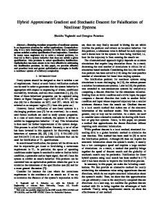
We have implemented our experiments in M ATLAB [16]. We used the CVODES ordinary differential equation solver from S UNDIALS [17] to compute the performance and the sensitivity for the simple system dynamics, and we used the dde23 solver [18] in M ATLAB for simulating the complex system dynamics that contain delay differential equations. For the experiments, we apply our approach with maximum of 1000 simulations. We compare the results of our approach with the Simulated Annealing (SA) optimization implementation in S-TaLiRo [19]. For SA, we use the same random initial input signal that was used to start the functional gradient descent method, and we limit the maximum number of simulations with 1000. We utilize only the complex dynamics of the system in the SA optimization. For comparison, we executed 190 experiments in total with our approach and with SA. In 167 of 190, i.e., in 87.9% of the executed experiments, the proposed functional gradient descent method achieved a smaller worst-case performance on the complex dynamics of the system compared to the SA optimization. The average of the explored minimum worst-case performance is −0.6532 with our approach and −0.6363 with SA. When all experiment results are considered, although the difference is negligibly small, the minimum worst-case performance found with our approach (−0.6551) was also smaller than the one found by SA (−0.6550). In Fig. 3, there is an entry (a blue star) for each experiment. Each entry represents how much the achieved

40

60

80

100

120

140

160

180

Initial and Final Acceleration Input for Dummy Vehicle

0.4

u initial

0.2

u final

0 -0.2 -0.4

0

50

Performance

100 t (s)

150

200

Initial and Final Performance

0 -0.2

Perf. Perf.

-0.4

initial final

-0.6 -0.8

0

50

100

150

200

t (s)

Fig. 4. Dummy vehicle acceleration and resulting worst-case performance

minimum worst-case performance value by the SA is larger than the achieved minimum worst-case performance value by our approach for an experiment. Hence, the positive values (i.e., the entries above the horizontal red line drawn at 0) are from the experiments where our approach outperformed SA, and the distance to 0 is a measure of how much it performed better then SA. Our approach outperforms SA in most of the experiments. Furthermore, the average performance improvement from our method is larger than the average performance improvement in the cases when SA outperforms our method. The initial random acceleration input, the resulting input after functional gradient descent, and the corresponding performance through the simulation trajectory are shown in Fig. 4. The figure is from the descent experiment which achieved the overall minimum worst-case performance. Figure 5 shows the accelerations of the vehicles for the input signal given in Fig. 4. Comparing this test case with the original stop and go scenario, the maximum absolute jerk 0.6551 m/s3 measured with this test case is larger than Vehicle Accelerations

0.5

a (m/s 2 )

C. Experiment Results

20

Fig. 3. Comparison of the proposed approach with Simulated Annealing using the difference in achieved minimum worst-case performance values

B. Stop and Go Scenario We aim to automatically create a scenario to find worstcase performance of P-FRACC and compare it to the original stop and go scenario from Mullakkal-Babu et al. [15]. Our experimental setup is similar to the original setup described above. For the sake of staying inside the targeted operation region, we limit the minimum and maximum acceleration of the dummy vehicle with −0.39 m/s2 and 0.39 m/s2 because these were the limit values in the original stop and go scenario. The accelerations of the vehicles simulated with the high-fidelity model in this scenario are shown in Fig. 2.

0

Experiment #

u (m/s2)

where s∆ (t−τs ) = min(s(t−τs )−s0 −vV (t−τs )td , (vdes − vV (t − τs ))td ). Furthermore, in the high-fidelity model, the velocity for the vehicles saturate at minimum and maximum velocities. Thus, applying functional gradient descent on the complex system dynamics is difficult due to the delay differential equations, the hybrid nature of the controller, and nonlinearities introduced for realism.

adummy avut1

0 -0.5

0

50

100

150

200

t (s)

Fig. 5.

Accelerations of vehicles under updated input

the maximum absolute jerk 0.3232 m/s3 we have measured with the original stop and go scenario. Because of possible differences in implementation details and in the differential equation solvers, some numerical differences may exist between our results and those of Mullakkal-Babu et al. [15]. The MAJ value 0.3232 m/s3 we have measured is approximately 10 times larger than the results reported by Mullakkal-Babu et al. because they do not normalize their consecutive acceleration values by the time step 0.1 s in the jerk computations. V. C ONCLUSIONS & D ISCUSSION For generating optimal test cases, we presented a functional gradient descent approach that uses simplistic yet analytically tractable dynamics to efficiently search more realistic dynamics of a complex system. As a case study, we implemented a full-range adaptive cruise control from the literature and utilized our approach for automatically generating test cases for exploring the worst-case performance of the controller within the boundaries of a target scenario. The results of our case study show that simple, yet sufficiently realistic, dynamical equations for the system under test can be used with a functional gradient descent method to search over more realistic complex dynamics of the actual system. The results of our method were better than those from Simulated Annealing, a proven metaheuristic for global optimization. However, we are not claiming that our approach is superior to SA optimization for every application. Rather, our case study shows that when simplified dynamics of a system are available, satisfactory optimization results can be obtained without the process of tuning SA parameters. Furthermore, our study shows that automated test-case generation can create more challenging test cases than the human-generated ones that are traditionally used in the literature, and these test cases will provide better insights into the performance of controllers under test. The work by Abbas et al. [20] defines a conformance metric for measuring the closeness of systems and methods to approximate this conformance. A formal analysis of closeness of the simple dynamics to the real system dynamics can be utilized to develop an approach for a better guided descent computation. However, in many cases we cannot have formal notions of distance between models as for example in modelorder reduction or approximate bisimulations. Another promising research direction is to combine our optimal trajectory generation approach with multi-fidelity optimization methods like those from Xu et al. [10], [11] and others [12], [21], [22]. In our method, the low-fidelity model is used to prioritize descent directions in a functional gradient descent. An alternative approach, for instance, is to mix high and low fidelity models to choose the best functional gradient descent directions, and existing multi-fidelity optimization methods may be well suited for this task. R EFERENCES [1] M. Maurer and H. Winner, Automotive systems engineering. Springer, 2013.

[2] K. Bengler, K. Dietmayer, B. Farber, M. Maurer, C. Stiller, and H. Winner, “Three decades of driver assistance systems: Review and future perspectives,” Intelligent Transportation Systems Magazine, IEEE, vol. 6, no. 4, pp. 6–22, 2014. [3] J. Kapinski, J. V. Deshmukh, X. Jin, H. Ito, and K. Butts, “Simulationbased approaches for verification of embedded control systems: An overview of traditional and advanced modeling, testing, and verification techniques,” IEEE Control Systems Magazine, vol. 36, no. 6, pp. 45–64, 2016. [4] C. E. Tuncali, T. P. Pavlic, and G. Fainekos, “Utilizing s-taliro as an automatic test generation framework for autonomous vehicles,” in Intelligent Transportation Systems (ITSC), 2016 IEEE 19th International Conference on. IEEE, 2016, pp. 1470–1475. [5] Y. Annpureddy, C. Liu, G. Fainekos, and S. Sankaranarayanan, “STaLiRo: A tool for temporal logic falsification for hybrid systems,” in International Conference on Tools and Algorithms for the Construction and Analysis of Systems. Springer, 2011, pp. 254–257. [6] H. Abbas, A. Winn, G. Fainekos, and A. A. Julius, “Functional gradient descent method for metric temporal logic specifications,” in American Control Conference (ACC), 2014. IEEE, 2014. [7] S. Yaghoubi and G. Fainekos, “Hybrid approximate gradient and stochastic descent for falsification of nonlinear systems,” in American Control Conference (ACC), 2017. [8] A. K. Winn and A. A. Julius, “Optimization of human generated trajectories for safety controller synthesis,” in American Control Conference (ACC). IEEE, 2013, pp. 4374–4379. [9] A. Melikyan, N. Hovakimyan, and Y. Ikeda, “Dynamic programming approach to a minimum distance optimal control problem,” in Proceedings of the 42nd IEEE Conference on Decision and Control, 2003. [10] J. Xu, S. Zhang, E. Huang, C.-H. Chen, L. H. Lee, and N. Celik, “An ordinal transformation framework for multi-fidelity simulation optimization,” in Automation Science and Engineering (CASE), 2014 IEEE International Conference on. IEEE, 2014, pp. 385–390. [11] ——, “MO2TOS: Multi-fidelity optimization with ordinal transformation and optimal sampling,” Asia-Pacific Journal of Operational Research, vol. 33, no. 03, 2016. [12] H. Li, Y. Li, L. H. Lee, E. P. Chew, G. Pedrielli, and C.-H. Chen, “Multi-objective multi-fidelity optimization with ordinal transformation and optimal sampling,” in Proceedings of the Winter Simulation Conference. IEEE Press, 2015, pp. 3737–3748. [13] Y. Eldar, M. Lindenbaum, M. Porat, and Y. Y. Zeevi, “The farthest point strategy for progressive image sampling,” IEEE Transactions on Image Processing, vol. 6, no. 9, pp. 1305–1315, 1997. [14] H. Abbas, G. Fainekos, S. Sankaranarayanan, F. Ivanˇci´c, and A. Gupta, “Probabilistic temporal logic falsification of cyber-physical systems,” ACM Transactions on Embedded Computing Systems (TECS), vol. 12, no. 2s, p. 95, 2013. [15] F. A. Mullakkal-Babu, M. Wang, B. van Arem, and R. Happee, “Design and analysis of full range adaptive cruise control with integrated collision a voidance strategy,” in Intelligent Transportation Systems (ITSC), 2016 IEEE 19th International Conference on. IEEE, 2016. [16] MATLAB, version 9.0.0 (R2016a). Natick, Massachusetts: The MathWorks Inc., 2016. [17] A. C. Hindmarsh, P. N. Brown, K. E. Grant, S. L. Lee, R. Serban, D. E. Shumaker, and C. S. Woodward, “SUNDIALS: Suite of nonlinear and differential/algebraic equation solvers,” ACM Transactions on Mathematical Software (TOMS), vol. 31, no. 3, pp. 363–396, 2005. [18] L. F. Shampine and S. Thompson, “Solving ddes in matlab,” Applied Numerical Mathematics, vol. 37, no. 4, pp. 441–458, 2001. [19] H. Abbas and G. Fainekos, “Convergence proofs for simulated annealing falsification of safety properties,” in Communication, Control, and Computing (Allerton), 2012 50th Annual Allerton Conference on. IEEE, 2012, pp. 1594–1601. [20] H. Abbas, H. Mittelmann, and G. Fainekos, “Formal property verification in a conformance testing framework,” in Formal methods and models for codesign (memocode), 2014 twelfth acm/ieee international conference on. IEEE, 2014, pp. 155–164. [21] R. Chen, J. Xu, S. Zhang, C.-H. Chen, and L. H. Lee, “An effective learning procedure for multi-fidelity simulation optimization with ordinal transformation,” in Automation Science and Engineering (CASE), 2015 IEEE International Conference on. IEEE, 2015, pp. 702–707. [22] E. Huang, J. Xu, S. Zhang, and C.-H. Chen, “Multi-fidelity model integration for engineering design,” Procedia Computer Science, vol. 44, pp. 336–344, 2015.