Fractal Image Compression Michael F. Barnsley
The top-selling multimedia encyclopedia Encarta, published by Microsoft Corporation, includes on one CD-ROM seven thousand color photographs which may be viewed interactively on a computer screen. The images are diverse; they are of buildings, musical instruments, people’s faces, baseball bats, ferns, etc. What most users do not know is that all of these photographs are based on fractals and that they represent a (seemingly magical) practical success of mathematics. Research on fractal image compression evolved from the mathematical ferment on chaos and fractals in the years 1978–1985 and in particular on the resurgence of interest in Julia sets and dynamical systems. Here I describe briefly some of the underlying ideas. Following Hutchinson [7], see also [5], consider first a finite set of contraction mappings wi , each with contractivity factor s < 1 , taking a compact metric space X into itself, i = 1, 2, . . . N . Such a setup is called an iterated function system (IFS), [1]. Use this IFS to construct a mapping W from the space H of nonempty compact subsets of X into itself by defining, in the self-explanatory notation,
Michael F. Barnsley is chief science and technology officer, Iterated Systems, Inc., Norcross, GA, and adjunct professor of mathematics, University of New South Wales, Australia. His e-mail address is Mbarnsley@ aol.com.
JUNE 1996
W (B) =
N [
wi (B)
for all B ∈ H.
i=1
Then W is a contraction mapping, with contractivity factor s < 1 , with respect to the Hausdorff metric h on H , defined as
h(A, B) = Max{d(A, B), d(B, A)} for all A, B ∈ H, where
d(A, B) = Max{d(x, B) : x ∈ A} for all A, B ∈ H,
with
d(x, B) =Min{d(x, y) : y ∈ B} for all x ∈ X, B ∈ H.
Moreover, H endowed with h is complete. In this setting W admits a unique fixed point; that is, there is exactly one nonempty compact subset A of X such that A = W (A) . A is called the attractor of the IFS. Now, following [3], suppose that X is a suitably large subset of R2 and that each of the transformations wi is an affine map expressed by six parameters,
w (x, y) = (ax + by + e, cx + dy + f ). Then the corresponding attractor is uniquely specified by the sets of numbers a, b, c, d, e, f ,…which describe the maps. Given NOTICES
OF THE
AMS
657
So how is a photograph, such as that shown in Figure 2, computed? First the theory of IFS is extended to local functions wi such that wi−1 : Di → Ri where the domains Di and ranges Ri are subsets of X , for i = 1, 2, . . . , N . Associated with an IFS of such functions we define
Wloc (B) =
N [
wi (Ri ∩ B)
for all B ∈ H.
i=1
Figure 1. One of the seven thousand fractal transform photographs from Microsoft Encarta. © Microsoft Corporation. a “black and white” image, which we model as a (compact nonempty) subset T of R2, we can choose the coefficients in an IFS of affine maps so that its attractor is an approximation to T. To achieve this, we seek coefficients for the mappings wi so that
h(T ,
N [
wi (T ))
i=1
is suitably small. For the contractivity of W implies the estimate [2]
(1)
h(T , A) ≤ (1 − s)−1 h(T ,
N [
wi (T )),
i=1
which tells us that if T is close to W (T ), then the attractor cannot be far away either. For example, the well-known “Barnsley” fern represents the attractor of an IFS of four affine maps which were chosen so that a fern image T was mapped approximately to itself under the corresponding W ; see [2] for more details. In this manner a fern subset of R2 may be encoded using 24 bytes of data, namely, four maps each requiring six parameters, each represented by an integer in the interval [0, 255]. 658
NOTICES
OF THE
AMS
Under appropriate side conditions, such operators continue to be contractive and to admit estimates of the character of Equation (1). Such is the case in the following setup. A grayscale photograph image may be modelled as the graph G ⊂ R3 of a function f : S → R that represents the intensity or brightness of the image on its support S ⊂ R2. Then one seeks a local IFS of contractive affine maps on R3 such that Wloc (G) approximates G and such that the projections Pi of the domains Di form a partition of S . In a typical implementation S is a rectangle and the Pi ’s are square tiles. For each i, to find a suitable contractive mapping wi , one searches in a digital computer implementation for the best match among some set of affine transformations between wi (Ri ∩ G) and the portion of G that lies above Pi , measured, say, by the minimum root-mean-square error. The coefficients and other descriptors of the selected local IFS are called a fractal transform of G ; its attractor ˜ for G . provides a succinct approximation G Figures 2, 3, and 4 provide a simple illustration of fractal compression. Figure 2 shows the original digital image of Balloon, which is of dimensions 512 pixels by 512 pixels, with 256 gray levels at each pixel. Figure 3 shows the same image after fractal compression, carried out as follows: each tile Pi (i = 0, 1, . . . , 16383) consists of a square of dimensions 4 pixels by 4 pixels, with the lower left corner of Pi located at pixel (j, k) where j = i mod 512 and k is the integer part of i/512 . The contractive transformations wi are chosen to be affine, of the form
wi (x, y, z) = (Ai (x, y), 0.75z + ci ), where Ai maps some square, in the support of the image, of dimensions 8 pixels by 8 pixels onto Pi . Each Ai is a similitude of contractivity factor 0.5. The origin of coordinates is at the lower left-hand corner of the image, and the z direction corresponds to intensity. The allowed squares are all of those with lower left corner at (2 · p, 2 · q) with p, q ∈ {0, 1, . . . , 251} and sides parallel to the axes, each of the eight possible isometries being admitted. The intensity coefficients ci are restricted to lie in the set {−256, −255, . . . , 255} . The set of allowed affine transformations associated with each tile Pi can be represented using 26 bits of data. The VOLUME 43, NUMBER 6
Figure 2. Original 512 x 512 grayscale image, with 256 gray levels for each pixel, before fractal compression. © Louisa Barnsley. part of the original associated with a single tile requires 128 bits of data; thus the fractal transform file is approximately one fifth the size of the original; the decompressed image computed from the fractal file is shown in Figure 3. In Figure 4 we show the result of restricting the choices for p and q so that the allowed squares associated with tile Pi typically lie very close to Pi ; for JUNE 1996
example, in the black regions Ai (Pi ) is simply a square of twice the size of Pi , centered on the center of Pi : an average of 3 bits is used to represent p and q together, the previously cited 26 bits is reduced to 15 bits on average, and the fractal transform file is approximately one eighth the size of the original. Correlations among the coefficients may be exploited by a standard lossNOTICES
OF THE
AMS
659
Figure 3. This shows the result of applying fractal compression and decompression to the image displayed in Figure 2. less compression technique such as Huffman encoding to reduce file sizes further. Figure 5 shows the result of a fractal zoom, whereby the attractor is computed at higher resolution than in the original: the fractal transform file associated with Figure 3 is decompressed so that each 4 × 4 block in the original image corresponds to an 8 × 8 block here. Illustrative source code for 660
NOTICES
OF THE
AMS
computing such fractal transforms is provided in [4] and [6]. Software and hardware engineers at Iterated Systems and researchers in many academic institutions [6] continue to develop more sophisticated methods and successive generations of products for computing attractors ever closer to true resolution-independent pictures. VOLUME 43, NUMBER 6
Figure 4. This shows the result of applying fractal compression and decompression to the image displayed in Figure 2, at a higher compression ratio than in Figure 3. See text.
Acknowledgments This work developed from basic research carried out in the School of Mathematics at Georgia Institute of Technology during the period 1979–1988; our group included Steven Demko, Jeffrey Geronimo, John Elton, Andrew Harrington, Mark Berger, and Alan Sloan. Graduate students who later joined the fray included Douglas JUNE 1996
Hardin, Els Withers, John Herndon, Peter Massopust, Arnaud Jacquin, and Laurie Reuter. Figures 3, 4, and 5 were computed by Ning Lu. References [1] M. F. Barnsley and S. G. Demko, Iterated function systems and the global construction of fractals, Proc. Roy. Soc. London A399 (1985), 2433–275.
NOTICES
OF THE
AMS
661
Figure 5. Fractal zoom on Figure 3 obtained by computing the attractor of the fractal transform at twice the resolution of the original. [2] M. F. Barnsley, V. Ervin, D. Hardin, and J. Lancaster, Solution of an inverse problem for fractals and other sets, Proc. Nat. Acad. Sci. 83 (1985), 1975–1977. [3] M. F. Barnsley, Fractals everywhere, Academic Press, Boston, 1988. [4] M. F. Barnsley and L. P. Hurd, Fractal image compression, A. K. Peters, Boston, 1992. [5] P. M. Diaconis and M. Shashahani, Products of random matrices and computer image generation, Contemp. Math. 50 (1986), 173–182.
662
NOTICES
OF THE
AMS
[6] Y. Fisher, Fractal image compression, SpringerVerlag, New York, 1995. [7] J. Hutchinson, Fractals and self-similarity, Indiana Univ. J. Math. 30 (1981), 713–747.
VOLUME 43, NUMBER6