FPTAS’s for Trimming Weighted Trees
★
Mingyu Xiao1 , Takuro Fukunaga2 , and Hiroshi Nagamochi2 1 2
School of Computer Science and Engineering, University of Electronic Science and Technology of China, China,
[email protected] Department of Applied Mathematics and Physics, Graduate School of Informatics, Kyoto University, Japan, {takuro,nag}@amp.i.kyoto-u.ac.jp
Abstract. Given a tree with nonnegative edge cost and nonnegative vertex weight, and a number 𝑘 ≥ 0, we consider the following four cut problems: cutting vertices of weight at most or at least 𝑘 from the tree by deleting some edges such that the remaining part of the graph is still a tree and the total cost of the edges being deleted is minimized or maximized. The MinMstCut problem (cut vertices of weight at most 𝑘 and minimize the total cost of the edges being deleted) can be solved in linear time and space and the other three problems are NP-hard. In this paper, we design an 𝑂(𝑛𝑙/𝜀)-time 𝑂(𝑙2 /𝜀 + 𝑛)-space algorithm for MaxMstCut, and 𝑂(𝑛𝑙(1/𝜀 + log 𝑛))-time 𝑂(𝑙2 /𝜀 + 𝑛)-space algorithms for the other two problems, MinLstCut and MaxLstCut, where 𝑛 is the number of vertices in the tree, 𝑙 the number of leaves, and 𝜀 > 0 the prescribed error bound. Key words.
1
Graph Cut, FPTAS, Tree, Tree Knapsack
Introduction
Given an undirected tree 𝐺 = (𝑉, 𝐸) with a nonnegative vertex weight 𝑤(𝑣), 𝑣 ∈ 𝑉 and a nonnegative edge cost 𝑐(𝑒), 𝑒 ∈ 𝐸, and a nonnegative number 𝑘 ≥ 0, the maximum cutting vertices of weight at most 𝑘 problem (MaxMstCut) is to find a nonempty and proper subset 𝑋 of 𝑉 that maximizes the total cost of edges with exact one endpoint in 𝑋 under the constraint that (i) the subgraph 𝐺[𝑉 −𝑋] induced by 𝑉 − 𝑋 is connected and (ii) the total weight of vertices in 𝑋 is at most 𝑘. Analogously, we also define MaxLstCut, MinMstCut and MinLstCut, by replacing “maximizes” with “minimizes” or replacing “at most” with “at least” in the definition. If 𝐺 is a rooted tree, then we impose the third constraint that the root is contained in the subgraph 𝐺[𝑉 − 𝑋] in finding a solution 𝑋. These problems are also called the cutting 𝑘 vertices (or vertices of weight 𝑘) problem in some references. In this paper, we mainly study algorithms for the above four cut problems in rooted and unrooted trees. In our algorithms, we may compute a solution 𝑋 ⊂ 𝑉 by identifying the corresponding set 𝐶 = 𝐸(𝑋, 𝑉 − 𝑋) of edges joining 𝑋 and 𝑉 − 𝑋, called cut set. ★
A preliminary version of this paper was presented in the 4th international frontiers of algorithmics workshop (FAW 2010) and appeared in [15].
2
Mingyu Xiao, Takuro Fukunaga, and Hiroshi Nagamochi
Graph cut problems have great applications and have been extensively studied in the literature. The minimum cut problem is regarded as a basic problem among this kind of problems. Many extensions of the classical minimum cut problem, including the multi-way cut problem [3, 13], the balanced cut problem [5] and the cutting 𝑘 vertices problem [4], are also important and fundamental problems. The multi-way cut problem extends the minimum cut problem in a way of partitioning the graph into more than two components. The balanced cut and cutting 𝑘 vertices problems are to find an optimal cut under some constraints on the size of the two parts of the cut. These two problems have similar requirement. However, the balanced cut problem is to deal with the case of almost balanced sizes of the two sides of the cut, while the cutting 𝑘 vertices problem is more to consider cuts with one small side. Although the minimum cut problem can be solved in polynomial time by flow and other techniques, most extended cut problems are NP-hard. Few “positive” results on the cutting 𝑘 vertices problem are known. Considering the hardness of the problems, we study the four cut problems MaxMstCut, MaxLstCut, MinMstCut and MinLstCut in the graphs restricted to trees. These problems in trees are still important to be investigated, since they naturally generate the famous knapsack problem from several ways. In fact, the cut problems in rooted trees are related to some special cases of the precedence constraint knapsack problem (PCKP) [7, 9]. In PCKP, a directed acyclic graph is given, each vertex in the graph is regarded as an item to be selected into the knapsack, and if a vertex is selected into the knapsack then all its ancestors (vertices having a direct path to the vertex) must also be selected into the knapsack. MaxMstCut (resp., MinLstCut) can model the precedence constraint knapsack problem in rooted trees with all edges directed toward the root (resp., the leaves), which is called the in-tree (resp., out-tree) knapsack problems [2, 7]. As a prior work on MinLstCut in rooted trees, there exists a (4/3 + 𝜖)approximation algorithm for the generalized partial totally unimodular cover problem with any 𝜖 > 0, presented by K¨onemann, Parekh and Segev [10]. Consider the matrix, whose rows are corresponding to the vertices and columns corresponding to the edges, such that its (𝑖, 𝑗)-th component is 1 if the 𝑖-th vertex is a descendant of the 𝑗-th edge, and 0 otherwise. If we order the vertices by DFS, then 1’s appear consecutively in each column. Such a matrix is known to be totally unimodular. Although we do not give a formulation of the partial totally unimodular cover problem, this observation indicates that MinLstCut is contained by their problem. Another related work is the algorithms for the tree knapsack problems. Cho and Shaw presented a depth-first dynamic programming algorithm for the out-tree knapsack problem in [2] that can be modified to get an 𝑂(𝑛(𝑊 − 𝑘))-time pseudo polynomial-time algorithm for MinLstCut in rooted trees, where 𝑊 is the total weight of all vertices in the tree. This pseudo polynomial-time algorithm can also be used to derive approximation schemes, but the running time depends on 𝑊 . Johnson and Niemi [7] designed several algorithms for two different tree knapsack problems. Their 𝑂(𝑛3 /𝜀)-time FPTAS (fully polynomial-time approximation scheme) for the in-tree knapsack problem
FPTAS’s for Trimming Weighted Trees
3
can solve MaxMstCut in rooted trees in the same time. There are few nontrivial results on the problems in unrooted trees. In this paper, except showing that MinMstCut in trees can be solved in linear time and space easily, we present: (i) 𝑂(𝑛𝑙/𝜀)-time 𝑂(𝑙2 /𝜀 + 𝑛)-space FPTAS’s for MaxMstCut in rooted and unrooted trees; (ii) 𝑂(𝑛𝑙(1/𝜀 + log 𝑛))-time 𝑂(𝑙2 /𝜀 + 𝑛)-space FPTAS’s for MinLstCut and MaxLstCut in rooted and unrooted trees. The rest of the paper is organized as follows. Section 2 gives our notation system. Section 3 considers the hardness of the problems. Section 4 presents pseudo polynomial-time algorithms that will be used to design FPTAS’s. Section 5 presents FPTAS for MaxMstCut in rooted trees and Section 6 presents FPTAS’s for MinLstCut and MaxLstCut in rooted trees. Section 7 designs FPTAS’s for MaxMstCut, MinLstCut and MaxLstCut in unrooted trees. Finally Section 8 makes some concluding remarks.
2
Preliminaries
Let ℜ+ denote the set of positive reals, and let ℜ∗ = ℜ+ ∪ {0}. We may denote by 𝑉 (𝐺) and 𝐸(𝐺) the sets of vertices and edges of an undirected graph 𝐺, respectively. For a graph 𝐺 = (𝑉, 𝐸) and a subset 𝑋 ⊆ 𝑉 , let 𝐺[𝑋] denote the subgraph of 𝐺 induced by the vertices in 𝑋, and let 𝐸(𝑋, 𝑉 − 𝑋) denote the set of edges with one endpoint in 𝑋 and the other in 𝑉 − 𝑋. For ∑ a vertex weight 𝑤 : 𝑉 → ℜ∗ ∑ and an edge cost 𝑐 : 𝐸 → ℜ∗ , let 𝑤(𝑋) denote 𝑣∈𝑋 𝑤(𝑣) and 𝑐(𝑋) denote 𝑒∈𝐸(𝑋,𝑉 −𝑋) 𝑐(𝑒), respectively. Given an unrooted tree 𝐺 and a vertex 𝑟 in it, we use 𝐺𝑟 to denote the rooted tree obtained from 𝐺 by choosing 𝑟 as the root. In a rooted tree, let 𝐷(𝑣) (resp., 𝐴(𝑣)) denote the set of descendants (resp., ancestors) of a vertex 𝑣, where 𝑣 ∈ 𝐷(𝑣) and 𝑣 ∈ 𝐴(𝑣). Denote the edge sets in the induced graphs 𝐺[𝐷(𝑣)] and 𝐺[𝐴(𝑣)] by 𝐸𝐷 (𝑣) and 𝐸𝐴 (𝑣), respectively. Let 𝑒𝑝 (𝑣) denote the edge joining 𝑣 and its parent. For each edge 𝑒 = (𝑢, 𝑣), where 𝑢 is the parent of 𝑣, define 𝐷(𝑒) and 𝐸𝐷 (𝑒) to be 𝐷(𝑣) and 𝐸𝐷 (𝑣), respectively. A set 𝑋 is called root-connecting if 𝐺[𝑉 − 𝑋] is connected and contains the root. We use 𝑛 and 𝑙 to denote the number of vertices and the number of leaves (i.e., vertices of degree 1) in the graph respectively. To distinguish edge weight with vertex weight, we say edge cost instead of edge weight. A special case of our cut problems is that the weight of vertices in the graph can only be 0 or 1. We will call the problems under this constraint the terminal case. We may call vertices 𝑣 with 𝑤(𝑣) = 1 terminals, and use 𝑇 to denote the set of terminals in the graph and let 𝑡 = ∣𝑇 ∣.
3 3.1
Computational Complexity In General Graphs
First, we study the hardness of our cut problems in general graphs. We consider the terminal case of the problems in nonnegative edge-cost graphs without the
4
Mingyu Xiao, Takuro Fukunaga, and Hiroshi Nagamochi
constraint (i) on the connectivity of 𝐺[𝑉 − 𝑋], where we can assume that given graphs are complete by introducing a new edge with cost 0 to each pair of nonadjacent vertices. Thus we treat our problems in complete graphs. For terminal cases, it may also be interesting to study the exact version of the problems: cutting exact 𝑘 terminals away from the graph by minimizing (maximizing) the cost of the cut. We use MinExtCut and MaxExtCut to denote these two problems. They will also be considered later. Since the maximum cut problem is a well-known NP-hard problem, we know that terminal MaxMstCut, MaxLstCut and MaxExtCut are NP-hard. We will pay more attention to the minimum version of the problems. In both terminal MinMstCut and MinLstCut, the target 𝑘 should be less than ∣𝑇 ∣/2, otherwise it is no meaning to distinguish them. It is easy to see that when 𝑘 is a constant, terminal MinMstCut, MinLstCut and MinExtCut are polynomial-time solvable as we can exhaustively search for all 𝑘 (or at most 𝑘)-terminal groups (For MinLstCut, we will find a minimum cut in each graph obtained by contracting a 𝑘-terminal group into a single terminal). When 𝑘 is part of input, it is also easy to show the NP-hardness of terminal MinExtCut by reducing from the balanced cut problem [1]. Marx [11] also studied the hardness of terminal MinExtCut from the Parameterized Complexity view. He proved that the problem is W[1]-hard, even when both 𝑘 and size of the corresponding cut set are taken as parameters, which shows the corresponding parameterized problem unlikely has any parameterized algorithm. Terminal MinExtCut remains NP-hard even if 𝑘 ≤ ∣𝑇 ∣/2, and this implies that terminal MinLstCut is NP-hard, because a terminal MinExtCut instance with 𝑘 ≤ ∣𝑇 ∣/2 can be polynomially reduced to a terminal MinLstCut instance by adding heavy edges between every two terminals so that any optimal solution of the terminal MinLstCut instance cuts exactly 𝑘 vertices away from the root. On the other hand, (terminal) MinMstCut is polynomially solvable by using an algorithm due to Nagamochi [12] for computing families of extreme sets (see Appendix A). 3.2
In Weighted Trees
Since the cut problems in general graphs are hard, we pay more attention to the scenarios where the graph is a tree. For the terminal case of the problems in trees, they can be solved in polynomial time by using dynamic programming (see Section 4). When vertex weight is nonnegative real number, MinLstCut and MaxMstCut in stars (trees having at most one vertex of degree > 1) are equal to the classical knapsack problem (each leaf in the star is corresponding to an item in the knapsack problem). For the hardness of MaxLstCut, we reduce another well-known NP-hard problem, the subset sum problem, to it. The subset sum problem is a special case of the knapsack problem, in which the profit of each item is equivalent to the weight of the item. Given a subset sum instance (𝑤(1), 𝑤(2), . . . , 𝑤(𝑛), ℎ) with 𝑛 items, where 𝑤(𝑖) is the weight of item 𝑖 and ℎ is the capacity of the knapsack, we construct a tree 𝑇 with 2𝑛 + 1 vertices in this way: Each item 𝑖 in the subset sum problem is corresponding to two vertices 𝑎𝑖
FPTAS’s for Trimming Weighted Trees
5
and 𝑏𝑖 in the tree. The weight of 𝑏𝑖 is 0 and the weight of 𝑎𝑖 is 𝑤(𝑖). There is also an auxiliary vertex 𝑣 with weight 0 in 𝑇 . There is an edge between 𝑎𝑖 and 𝑏𝑖 with cost 𝑤(𝑖) and an edge between 𝑎𝑖 and 𝑣 with cost 0. The target 𝑘 in the tree is set to be 𝑊 − ℎ, where 𝑊 is the total weight of items. Note that the cut set corresponding to an optimal solution to MaxLstCut in 𝑇 will contain exact one edge in {𝑎𝑖 𝑏𝑖 , 𝑎𝑖 𝑣} for each 𝑖. Then if item 𝑖 is selected into the knapsack, we include edge 𝑎𝑖 𝑏𝑖 into the cut set. Otherwise, we include edge 𝑎𝑖 𝑣 into the cut set. For each optimal solution to MaxLstCut we can also construct a solution to the knapsack problem. Therefore, we can prove the correctness of this reduction. MinMstCut is polynomial-time solvable in general graphs even without the constraint on the vertex weight. We further show that the problem can be solved in linear time when the graph is restricted to a tree. Note that the edge cost and vertex weight are nonnegative. The cut set corresponding to an optimal solution only contains one edge. We only need to identify a feasible edge with minimum cost. An edge 𝑒 in a rooted tree is a feasible edge if 𝑤(𝐷(𝑒)) ≤ 𝑘, and an edge 𝑒 in an unrooted tree is a feasible edge if at least one of the two component of 𝐺 − 𝑒 is of total vertex weight ≤ 𝑘. We can find all feasible edges in a DFS (For an unrooted tree, we arbitrarily select a vertex as the root and consider if min{𝑤(𝐷(𝑣)), 𝑊 − 𝑤(𝐷(𝑣))} ≤ 𝑘 for each vertex 𝑣). In the DFS, we only need to remember the feasible edge with minimum cost among all visited edges. Therefore, we can solve the problem in linear time and space. We will not discuss MinMstCut in the rest of the paper.
4
Pseudo Polynomial-time Algorithms
In this section, we give dynamic programming algorithms for our problems in rooted trees, which are pseudo polynomial-time algorithms and will be used to derive FPTAS’s. One technique we used to design the dynamic programming algorithms is called the “left-right” method for trees in [7]. To get the pseudo polynomial-time algorithms, we assume that all edge cost are integers in this section. In fact, our algorithm will find an optimal solution 𝑋 only when 𝑐(𝑋) ≤ 𝑞 holds for a prescribed threshold 𝑞. We order all the leaves in the tree according to a DFS (first visited has small index). Let 𝐿 = {𝑧1 , 𝑧2 , . . . , 𝑧𝑙 }, 𝑙 = ∣𝐿∣, be the set of leaves, where leaves 𝑧1 , 𝑧2 , . . . , 𝑧𝑙 appear from left to right in this order (see Fig. 1 for an illustration). To construct a root-connecting set 𝑋, if a vertex 𝑣 does not belong to 𝑋 (i.e., 𝑣 is not allowed to be cut away from the rooted tree), then all the edges in the path from 𝑣 to the root are not allowed to be deleted. Let 𝑉 ′ be the set of non-root vertices in the tree. For 0 ≤ 𝑖 ≤ 𝑙 and 0 ≤ 𝑗 ≤ 𝑞, define 𝒳 (𝑖, 𝑗) to be the set of all root-connecting sets 𝑋 ⊆ 𝑉 ′ that satisfy two constraints: 𝐿 ∩ 𝑋 ⊆ {𝑧1 , 𝑧2 , . . . , 𝑧𝑖 } (only the first 𝑖 leaves are allowed to be cut away); and 𝑐(𝑋) = 𝑗. We set { min{𝑤(𝑋) ∣ 𝑋 ∈ 𝒳 (𝑖, 𝑗)} for MaxMstCut 𝑂𝑃 𝑇 (𝑖, 𝑗) = max{𝑤(𝑋) ∣ 𝑋 ∈ 𝒳 (𝑖, 𝑗)} for MaxLstCut and MinLstCut.
6
Mingyu Xiao, Takuro Fukunaga, and Hiroshi Nagamochi root
e
z1
...... P
z2 z3 z4 α (e) = 3
Pi
i −1
zi −2
...... zi −1
zi
Fig. 1. An illustration of the rooted tree in our DP algorithm
Let 𝑋(𝑖, 𝑗) store a set 𝑋 ∈ 𝒳 (𝑖, 𝑗) attaining 𝑤(𝑋) = 𝑂𝑃 𝑇 (𝑖, 𝑗), where we let 𝑋(𝑖, 𝑗) =⊥ and 𝑂𝑃 𝑇 (𝑖, 𝑗) = ∞ if 𝒳 (𝑖, 𝑗) = ∅. Clearly for the maximum integer 𝑐0 such that 𝑂𝑃 𝑇 (𝑙, 𝑐0 ) ≤ 𝑘, 𝑋(𝑙, 𝑐0 ) is an optimal solution to MaxMstCut. Similarly for the maximum (resp., minimum) integer 𝑐0 such that 𝑂𝑃 𝑇 (𝑙, 𝑐0 ) ≥ 𝑘, 𝑋(𝑙, 𝑐0 ) is an optimal solution to MaxLstCut (resp., MinLstCut). We maintain a table of size (𝑙 + 1) × (𝑞 + 1) to store 𝑂𝑃 𝑇 (𝑖, 𝑗) and 𝑋(𝑖, 𝑗) for 0 ≤ 𝑖 ≤ 𝑙 and 0 ≤ 𝑗 ≤ 𝑞. To get a recursive formula among these, we consider a partition of the edge set 𝐸 into 𝑙 subsets 𝑃𝑖 = 𝐸𝐴 (𝑧𝑖 ) − 𝐸𝐴 (𝑧𝑖+1 ), 𝑖 = 1, 2, . . . , 𝑙, where we regard 𝐸𝐴 (𝑧𝑙+1 ) as ∅. Note that 𝑃𝑖 is the set of edges 𝑒 such that deleting 𝑒 cuts 𝑧𝑖 away without cutting 𝑧𝑖+1 away (see Fig. 1 for an illustration of 𝑃𝑖 ). Then, for any edge 𝑒 ∈ 𝑃𝑖 , deleting 𝑒 cuts away leaves 𝑧𝑎 , 𝑧𝑎+1 , . . . , 𝑧𝑖 with consecutive indices. Let 𝛼(𝑒) be the smallest index 𝑎 of the leaves in 𝑉 (𝑒). Then all values 𝑂𝑃 𝑇 (𝑖, 𝑗) and 𝑋(𝑖, 𝑗) for MaxMstCut can be computed by the recursive formula in Fig. 2. Algorithm DP for MaxLstCut and MinLstCut can be obtained by replacing the if condition in Step 2 with 𝑂𝑃 𝑇 (𝛼(𝑒)−1, 𝑗 − 𝑐(𝑒)) + 𝑤(𝑒) > 𝑂𝑃 𝑇 (𝑖, 𝑗) and modifying the choice of 𝑐0 in Step 3. Lemma 1. For a rooted tree 𝐺 with nonnegative integer edge cost and nonnegative vertex weight, Algorithm DP(𝐺, 𝑘, 𝑞) can be implemented to run in 𝑂(𝑞𝑛) time and 𝑂(𝑞𝑙 + 𝑛) space. Each iteration for an edge 𝑒 ∈ 𝑃𝑖 in the fourth line of Step 2 can be executed in 𝑂(1) time by representing 𝑋 = 𝑋(𝑖, 𝑗) as the edge set 𝐸(𝑋, 𝑉 − 𝑋) and updating 𝐸(𝑋, 𝑉 − 𝑋) by adding the edge 𝑒. Since {𝑃𝑖 ∣ 𝑖 = 1, 2, . . . , 𝑙} is a partition of the edge set 𝐸, each edge is considered only once for each fixed 𝑗 in the algorithm. Since 𝑗 runs from 1 to 𝑞, the running time of the algorithm is 𝑂(𝑞𝑛). The space of the algorithm is 𝑂(𝑞𝑙 + 𝑛). Since DP(𝐺, 𝑘, 𝑞) only computes 𝑂𝑃 𝑇 (𝑖, 𝑗) for 𝑗 from 0 to 𝑞, when the cost of an optimal solution is greater than 𝑞, DP(𝐺, 𝑘, 𝑞) cannot find an optimal solution.
FPTAS’s for Trimming Weighted Trees
7
Algorithm DP(𝐺, 𝑘, 𝑞) Input: A tree 𝐺 = (𝑉, 𝐸) rooted at a vertex 𝑟 with nonnegative integer edge cost 𝑐 and nonnegative vertex weight 𝑤, a number 𝑘 ≥ 0, and an integer 𝑝 ≥ 0. Output: A maximum cost root-connecting set 𝑋 such that 𝑤(𝑋) ≤ 𝑘 and 𝑐(𝑋) ≤ 𝑝, if any, or ⊥ otherwise. 1. For 𝑗 = 1 to 𝑞, do 𝑂𝑃 𝑇 (0, 𝑗) ←− ∞ and 𝑋(0, 𝑗) ←−⊥. For 𝑖 = 0 to 𝑙, do 𝑂𝑃 𝑇 (𝑖, 0) ←− 0 and 𝑋(𝑖, 0) ←− ∅. 2. For 𝑖 = 1 to 𝑙, do For 𝑗 = 1 to 𝑞, do 𝑂𝑃 𝑇 (𝑖, 𝑗) ←− 𝑂𝑃 𝑇 (𝑖 − 1, 𝑗) and 𝑋(𝑖, 𝑗) ←− 𝑋(𝑖 − 1, 𝑗). For each 𝑒 ∈ 𝑃𝑖 with 𝑐(𝑒) ≤ 𝑗, do If 𝑂𝑃 𝑇 (𝛼(𝑒)−1, 𝑗 − 𝑐(𝑒)) + 𝑤(𝑒) < 𝑂𝑃 𝑇 (𝑖, 𝑗), then 𝑂𝑃 𝑇 (𝑖, 𝑗) ←− 𝑂𝑃 𝑇 (𝛼(𝑒)−1, 𝑗 − 𝑐(𝑒)) + 𝑤(𝐷(𝑒)) and 𝑋(𝑖, 𝑗) ←− 𝑋(𝛼(𝑒)−1, 𝑗 − 𝑐(𝑒)) ∪ 𝐷(𝑒). 3. Let 𝑐0 be the maximum integer such that 𝑂𝑃 𝑇 (𝑙, 𝑐0 ) ≤ 𝑘. 4. Return 𝑋(𝑙, 𝑐0 ). Fig. 2. Algorithm DP(𝐺, 𝑘, 𝑞) for MaxMstCut
Note that the recursion in Fig. 2 can be rewritten to do over vertex weight instead of edge cost by maintaining a table of size (𝑙 + 1) × (𝑘 + 1) to store 𝑂𝑃 𝑇 ′ (𝑖, 𝑗) (and also 𝑋 ′ (𝑖, 𝑗)) for 0 ≤ 𝑖 ≤ 𝑙 and 0 ≤ 𝑗 ≤ 𝑘, where 𝑂𝑃 𝑇 ′ (𝑖, 𝑗) = max{𝑐(𝑋) ∣ 𝑋 ∈ 𝒳 ′ (𝑖, 𝑗)} and 𝒳 ′ (𝑖, 𝑗) is the set of all root-connecting sets 𝑋 ⊆ 𝑉 ′ that satisfy two constraints: 𝐿 ∩ 𝑋 ⊆ {𝑧1 , 𝑧2 , . . . , 𝑧𝑖 } and 𝑤(𝑋) = 𝑗. Then we can get running time bound 𝑂(𝑘𝑛) time and space bound 𝑂(𝑘𝑙 + 𝑛) for the modified algorithm (We also need to assume that all vertex weight are integers for this case). This also implies that the terminal case of our cut problems can be solved in 𝑂(𝑘𝑛) time and 𝑂(𝑘𝑙 + 𝑛) space.
5
FPTAS for MaxMstCut in Rooted Trees
First, we consider MaxMstCut in rooted trees and then extend our results to the problem in unrooted trees in Section 7. 5.1
Preprocesses
We show some conditions on edges that can be ruled out from a given instance of MaxMstCut. An edge 𝑒 is called an overload edge if 𝑤(𝐷(𝑒)) > 𝑘, i.e., the total weight of vertices cut away from the tree by deleting it exceeds 𝑘. Clearly, we can simply contract all overload edges to form the new rooted tree. A non-leaf edge 𝑒 is called a dominated edge if 𝑐(𝑒) is not larger than the total of 𝑐(𝑒′ ) of the child-edges 𝑒′ of 𝑒 (i.e., the edges in 𝐸𝐷 (𝑒) adjacent to 𝑒). Thus, for any rootconnecting set 𝑋 with a dominated edge 𝑒 = (𝑢, 𝑣) ∈ 𝐸(𝑋, 𝑉 −𝑋), where 𝑣 ∈ 𝑋, 𝑋 ′ = 𝑋 − {𝑣} satisfies 𝑐(𝑋 ′ ) ≥ 𝑐(𝑋) and 𝑤(𝑋 ′ ) ≤ 𝑤(𝑋) by nonnegativeness
8
Mingyu Xiao, Takuro Fukunaga, and Hiroshi Nagamochi
of 𝑐 and 𝑤, indicating that there is an optimal solution 𝑋 ∗ to MaxMstCut such that 𝑒 ∕∈ 𝐸(𝑋, 𝑉 − 𝑋). Hence we can also safely contract all dominated edges. This can be done in a bottom-up manner from leaves toward the root in linear time. Observe that, in a rooted tree with no dominated edges, for each non-root vertex 𝑣, 𝐷(𝑣) has the maximum cut cost 𝑐(𝐷(𝑣)) over all root-connecting sets 𝑋 ⊆ 𝐷(𝑣). 5.2
A
1 -Approximation 3
Algorithm
To design our FPTAS for MaxMstCut, we first give an 𝑂(𝑛 log 𝑙)-time 13 -approximation algorithm. The idea of the algorithm comes from a well-known greedy approximation algorithm for the knapsack problem, which is to greedily select items of the most dense. For each non-root vertex 𝑣 with 𝐷(𝑣) > 0, the density of 𝑣 is defined to be 𝜌(𝑣) = 𝑐(𝑒)/𝑤(𝐷(𝑣)), where 𝑒 = 𝑒𝑝 (𝑣). The simple approximation algorithm is presented in Fig. 3, where through out the computation, we use the density 𝜌(𝑣) of vertices 𝑣 in the graph obtained in Step 1, and never recompute new densities even after fixing some vertices as part of the current root-connecting set 𝑌 .
Algorithm Appro(𝐺, 𝑘) Input: A rooted tree 𝐺 = (𝑉, 𝐸) with nonnegative edge cost 𝑐 : 𝐸 → ℜ∗ and nonnegative vertex weight 𝑤 : 𝑉 → ℜ∗ and a number 𝑘 > 0. Output: A 13 -approximation solution to MaxMstCut in 𝐺. 1. Contract all overload and dominated edges. Let 𝑉 ′ be the set of non-root vertices in the resulting tree. Compute the density 𝜌. 2. 𝑌 ←− the union of sets 𝐷(𝑣) with 𝑤(𝐷(𝑣)) = 0 and 𝑣 ∈ 𝑉 ′ . 3. While 𝑉 ′ − 𝑌 ∕= ∅, do Select 𝑣 ∈ 𝑉 ′ −𝑌 such that 𝜌(𝑣) is maximized (possibly 𝑌 ∩𝐷(𝑣) ∕= ∅). If 𝑤(𝑌 ∪ 𝐷(𝑣)) ≤ 𝑘, then 𝑌 ←− 𝑌 ∪ 𝐷(𝑣). Else return one of 𝑌 and 𝐷(𝑣) that attains max{𝑐(𝑌 ), 𝑐(𝐷(𝑣))}, and halt. 4. Return 𝑌 . Fig. 3. Algorithm Appro(𝐺, 𝑘)
Lemma 2. Algorithm Appro(𝐺, 𝑘) is an 𝑂(𝑛 log 𝑙)-time 13 -approximation algorithm for MaxMstCut in rooted trees with nonnegative edge cost and nonnegative vertex weight. Proof. Since we have contracted all dominated edges, we know that there is an optimal root-connecting set 𝑋 ∗ contains all sets 𝐷(𝑣) with 𝑤(𝐷(𝑣)) = 0 in the tree. Then we can simply put them into the solution set directly. Next, if the algorithm stops at Step 4, it will return an optimal solution 𝑌 = 𝑉 ′ , since 𝑐(𝑉 ′ ) attains the maximum cut cost 𝑐(𝑋) over all root-connecting sets 𝑋.
FPTAS’s for Trimming Weighted Trees
9
Otherwise the algorithm will return 𝑌 or 𝐷(𝑣 ′ ) in Step 3, where 𝑣 ′ is the last vertex being selected in the algorithm. Note that 𝐷(𝑣 ′ ) is excluded from 𝑌 in the algorithm. Thus 𝑌 is a feasible solution when the algorithm halts. 𝐷(𝑣 ′ ) is also a feasible solution, because all overload edges are contracted in Step 1. Assume that 𝑋 ∗ is an optimal solution. We partition 𝑌 and 𝑋 ∗ into disjoint subsets: 𝑌 = 𝐷(𝑣1 )∪𝐷(𝑣2 )∪⋅ ⋅ ⋅∪𝐷(𝑣𝑦 ) and 𝑋 ∗ = 𝐷(𝑢1 )∪𝐷(𝑢2 )∪⋅ ⋅ ⋅∪𝐷(𝑢𝑥 ), where 𝑣𝑖 is not a descendent of any vertex in 𝑌 −{𝑣𝑖 } and 𝑢𝑖 is not a descendent of any vertex in 𝑋 ∗ − {𝑢𝑖 }. We further assume that {𝑣1 , . . . , 𝑣𝑦 } ∩ {𝑢1 , . . . , 𝑢𝑥 } = {𝑢1 , . . . , 𝑢ℎ }. Let 𝑋1 = 𝐷(𝑢1 ) ∪ 𝐷(𝑢2 ) ∪ ⋅ ⋅ ⋅ ∪ 𝐷(𝑢ℎ ) and 𝑋2 = 𝑋 ∗ − 𝑋1 = 𝐷(𝑢ℎ+1 ) ∪ ⋅ ⋅ ⋅ ∪ 𝐷(𝑢𝑥 ). Obviously, 𝑋1 ⊆ 𝑌 and 𝑋1 is still a feasible solution. By the nonnegativeness of 𝑐, 𝑐(𝑌 ) ≥ 𝑐(𝑋1 ). Since at the time when the algorithm selects 𝑣 ′ , no vertex in {𝑢ℎ+1 , . . . , 𝑢𝑥 } has been selected by the greedy strategy, we know that 𝜌(𝑣𝑖 ) ≥ 𝜌(𝑣 ′ ) ≥ 𝜌(𝑢𝑗 ) holds for any 𝑖 = 1, . . . , 𝑦 and 𝑗 = ℎ + 1, . . . , 𝑥. Since 𝑤(𝑌 ∪ 𝐷(𝑣 ′ )) > 𝑘 ≥ 𝑤(𝑋2 ), this implies that 𝑐(𝑌 ∪ 𝐷(𝑣 ′ )) > 𝑐(𝑋2 ). Hence we have 𝑐(𝑋 ∗ ) = 𝑐(𝑋1 ) + 𝑐(𝑋2 ) ≤ 𝑐(𝑌 ) + 𝑐(𝑌 ∪ 𝐷(𝑣 ′ )) ≤ 2𝑐(𝑌 ) + 𝑐(𝐷(𝑣 ′ )). Therefore, one of 𝑐(𝑌 ) and 𝑐(𝐷(𝑣 ′ )) must have cost at least 31 𝑐(𝑋 ∗ ). As for the running time, we only need to show that Step 3 can be done in 𝑂(𝑛 log 𝑙) time. First of all, we compute the densities of all vertices in the tree in a DFS. If a vertex 𝑣 has an ancestor 𝑢 such that 𝜌(𝑣) < 𝜌(𝑢), we say that 𝑣 is a weak vertex and 𝑒𝑝 (𝑣) a weak edge. Note that the algorithm will never select a weak vertex in Step 3. We can reduce the tree by contracting all weak edges. Detecting and contracting all weak edges can be done in a DFS. After reducing the tree, the tree has the monotonicity property: on any path from the root to a leaf, the vertex densities give a nonincreasing sequence. Then we can sort all the vertices according to their densities in 𝑂(𝑛 log 𝑙) time as we do in Mergesort. After sorting the vertices, we only need to select vertices according to the sorting list. Then we can do Step 3 in 𝑂(𝑛 log 𝑙) time. Note. This greedy algorithm can get approximation ratio 12 for the knapsack problem. Note that when the graph is a star, in the above proof we will have that 𝑐(𝑋2 ) ≤ 𝑐(𝑌 ∪{𝑣 ′ }−𝑋1 ) (since 𝑤(𝑌 ∪{𝑣 ′ }−𝑋1 ) > 𝑘 −𝑤(𝑋1 ) ≥ 𝑤(𝑋2 ) and 𝜌(𝑣𝑖 ) ≥ 𝜌(𝑣 ′ ) ≥ 𝜌(𝑢𝑗 ) for any 𝑖 = 1, . . . , 𝑦 and 𝑗 = ℎ + 1, . . . , 𝑥). Then 𝑐(𝑋 ∗ ) = 𝑐(𝑋1 )+𝑐(𝑋2 ) ≤ 𝑐(𝑌 )+𝑐({𝑣 ′ }). At least one of 𝑐(𝑌 ) and 𝑐({𝑣 ′ }) must have cost at least 12 𝑐(𝑋 ∗ ). Ibarra and Kim [6] also introduced an 𝑂(𝑛2 )-time 21 -approximation algorithm for MaxMstCut in rooted trees. In their algorithm, they will update the densities of vertices when each time selecting a vertex of maximum density and deleting it from the tree.3 We will use our 31 -approximation algorithm instead of their 12 -approximation algorithm, because we cannot improve the running time bound of our FPTAS by improving the approximation ratio from 13 to 21 , but will worsen the running time bound if the running time of the constant approximation algorithm changes from 𝑂(𝑛 log 𝑙) to 𝑂(𝑛2 ). 3
The correctness of the algorithm (Theorem 2 in [6]) was proved by assuming an important property (the fourth line of the proof of Theorem 2), the complete proof of which was omitted.
10
5.3
Mingyu Xiao, Takuro Fukunaga, and Hiroshi Nagamochi
The FPTAS
Next, we design the FPTAS for MaxMstCut. Let 𝑅 =Appro(𝐺, 𝑘). Algorithm DP(𝐺, 𝑘, 3𝑐(𝑅)) will find an optimal solution for our problem (assume that all edge costs are integers). If the cost of each edge is a small number, i.e., bounded by a polynomial of 𝑛, then DP(𝐺, 𝑘, 3𝑐(𝑅)) runs in polynomial time. To obtain an FPTAS, we scale the cost of each edge down to be bounded by a polynomial of 𝑛 and use Algorithm DP on the new instance to get a solution. By scaling with respect to the desired error 𝜀, we can get a solution with cost within (1−𝜀)𝑐(𝑋 ∗ ) and 𝑐(𝑋 ∗ ) in polynomial time with respect to both 𝑛 and 1/𝜀, where 𝑋 ∗ is an optimal solution to the original instance (𝐺, 𝑘). The FPTAS for MaxMstCut is described in Fig. 4. Algorithm Fptas1(𝐺, 𝑘, 𝜀) Input: A rooted tree 𝐺 = (𝑉, 𝐸) with nonnegative edge cost 𝑐 : 𝐸 → ℜ∗ and nonnegative vertex weight 𝑤 : 𝑉 → ℜ∗ , and two numbers 𝑘 ≥ 0 and 1 > 𝜀 > 0. Output: A (1 − 𝜀)-approximation solution to MaxMstCut. 1. 2. 3. 4.
𝑅 ←−Appro(𝐺, 𝑘) and 𝑔 ←− 𝑐(𝑅). If 𝑔 = 0, return 𝑅 as an optimal solution and halt. 𝑄 ←− 𝜀𝑔/𝑙 and replace 𝑐(𝑒) with 𝑐′ (𝑒) = ⌊𝑐(𝑒)/𝑄⌋ to get 𝐺′ . Return DP(𝐺′ , 𝑘, ⌊3𝑔/𝑄⌋). Fig. 4. Algorithm Fptas1(𝐺, 𝑘, 𝜀)
Theorem 1. For MaxMstCut in a rooted tree with nonnegative edge cost and nonnegative vertex weight, algorithm Fptas1(𝐺, 𝑘, 𝜀) runs in 𝑂(𝑛𝑙/𝜀) time and 𝑂(𝑙2 /𝜀 + 𝑛) space, and returns a root-connecting set 𝑌 such that 𝑐(𝑌 ) ≥ (1 − 𝜀)𝑐(𝑋 ∗ ),
(1)
where 𝑋 ∗ is an optimal solution to MaxMstCut. Proof. Since Appro(𝐺, 𝑘) runs in 𝑂(𝑛 log 𝑙) time and 𝑂(𝑛) space, and DP(𝐺′ , 𝑘, ⌊3𝑔/𝑄⌋) runs in 𝑂(3𝑔𝑛/𝑄) = 𝑂(𝑛𝑙/𝜀) time and 𝑂(3𝑔𝑙/𝑄 + 𝑛) = 𝑂(𝑙2 /𝜀 + 𝑛) space, we get the running time and space bounds. Next, we prove (1). It is clear that for any edge 𝑒, 0 ≤ 𝑐(𝑒) − 𝑄𝑐′ (𝑒) < 𝑄. Since the cardinality of any cut is at most the number 𝑙 of leaves in 𝐺, any root-connecting set 𝑋 ∕= ∅ satisfies ∣𝐸(𝑉 − 𝑋, 𝑋)∣ ≤ 𝑙 and 0 ≤ 𝑐(𝑋) − 𝑄𝑐′ (𝑋) < 𝑙𝑄. Since 𝑐′ (𝑋 ∗ ) ≤ ⌊𝑐(𝑋 ∗ )/𝑄⌋ ≤ ⌊3𝑔/𝑄⌋ holds, DP(𝐺′ , 𝑘, ⌊3𝑔/𝑄⌋) finds an optimal solution 𝑌 for the scaled instance, which satisfies 𝑐′ (𝑋 ∗ ) ≤ 𝑐′ (𝑌 ) ≤ ⌊3𝑔/𝑄⌋. Since 𝑐′ (𝑌 ) ≥ 𝑐′ (𝑋 ∗ ) ≥ 𝑔, we have 𝑐(𝑌 ) ≥ 𝑄𝑐′ (𝑌 ) ≥ 𝑄𝑐′ (𝑋 ∗ ) ≥ 𝑐(𝑋 ∗ ) − 𝑙𝑄 = 𝑐(𝑋 ∗ ) − 𝜀𝑔 ≥ (1 − 𝜀)𝑐(𝑋 ∗ ).
FPTAS’s for Trimming Weighted Trees
6
11
FPTAS’s for MinLstCut and MaxLstCut in Rooted Trees
We cannot directly extend the FPTAS for MaxMstCut in Section 5 to an FPTAS for MinLstCut or MaxLstCut in rooted trees, because we have no similar constant factor algorithm as Appro(𝐺, 𝑘) for MinLstCut or MaxLstCut. To get a constant factor algorithm, we will use a “rounding” technique [14]. This technique is used as a basic trick for deriving FPTAS’s for many problems. We will also use a new technique, called “binary search”, to get the finial FPTAS. In this section, we design the FPTAS for MinLstCut, which can also be modified to solve MaxLstCut. 6.1
The Preliminary Algorithm
First we present an algorithm Scaling for MinLstCut. Whether a given MinLstCut instance (𝐺, 𝑘) has an optimal solution 𝑋 ∗ with 𝑐(𝑋 ∗ ) = 0 or not can be tested in linear time by checking if 𝑤(𝑉 ′ ) ≥ 𝑘 for the set 𝑉 ′ of non-root vertices in the tree obtained by contracting all edges with positive costs. We here assume that 𝑐(𝑋 ∗ ) ≥ 𝑐min for the minimum 𝑐min of positive edge costs. Given an instance such that 𝑝 ≤ 𝑐(𝑋 ∗ ) for a positive number 𝑝 and a prescribed number 𝜀 > 0, algorithm Scaling will run in 𝑂(𝑙𝑛/𝜀) time and 𝑂(𝑙2 /𝜀 + 𝑛) space and return a feasible solution with value 𝑐(𝑌 ) satisfying (1 + 𝜀)𝑐(𝑋 ∗ ) ≥ 𝑐(𝑌 ), if 𝑐(𝑋 ∗ ) ≤ 2𝑝, or 𝑌 =⊥ if 𝑐(𝑋 ∗ ) > 2𝑝.
Algorithm Scaling(𝐺, 𝑘, 𝜀, 𝑝) Input: A rooted tree 𝐺 = (𝑉, 𝐸) with nonnegative edge cost 𝑐 : 𝐸 → 𝑅∗ and nonnegative vertex weight 𝑤 : 𝑉 → 𝑅∗ , and three numbers 𝑘 ≥ 0, 𝜀 > 0 and a number 𝑝 ≥ 𝑐min . Output: A feasible solution to MinLstCut, if any, or ⊥ otherwise. 1. 𝑄 ←− 𝜀𝑝/𝑙 and replace 𝑐(𝑒) with 𝑐′ (𝑒) = ⌊𝑐(𝑒)/𝑄⌋ to get 𝐺′ . 2. Return DP(𝐺′ , 𝑘, ⌊2𝑝/𝑄⌋). Fig. 5. Algorithm Scaling(𝐺, 𝑘, 𝜀, 𝑝)
By the definition of DP(𝐺′ , 𝑘, ⌊2𝑝/𝑄⌋) for MinLstCut, it will return a feasible solution 𝑌 such that 𝑐′ (𝑌 ) ≤ ⌊2𝑝/𝑄⌋ if any, or ⊥ otherwise. Note that if it returns ⊥ then we know 𝑐(𝑋 ∗ ) > 2𝑝 since 𝑐(𝑋 ∗ ) ≤ 2𝑝 implies 𝑐′ (𝑋 ∗ ) ≤ ⌊2𝑝/𝑄⌋. Assume 𝑝 ≤ 𝑐(𝑋 ∗ ) ≤ 2𝑝 and let 𝑌 = Scaling(𝐺, 𝑘, 𝜀, 𝑝). Analogously with the analysis of Theorem 1, we can prove that directly 𝑐(𝑌 ) ≤ 𝑄 ⋅ 𝑐′ (𝑌 ) ≤ 𝑄 ⋅ 𝑐′ (𝑋 ∗ ) ≤ 𝑐(𝑋 ∗ ) + 𝑙𝑄 = 𝑐(𝑋 ∗ ) + 𝜀𝑝. Hence if 𝑐(𝑋 ∗ ) ≥ 𝑝 then 𝑐(𝑌 ) ≤ (1+𝜀)𝑐(𝑋 ∗ ) holds. Therefore, Scaling(𝐺, 𝑘, 𝜀, 𝑝) works as claimed.
12
Mingyu Xiao, Takuro Fukunaga, and Hiroshi Nagamochi
To get an approximation scheme, we need to compute a value 𝑝∗ such that 𝑝 ≤ 𝑐(𝑋 ∗ ) ≤ 2𝑝∗ and call Scaling(𝐺, 𝑘, 𝜀, 𝑝∗ ). To detect such 𝑝∗ , we repeatedly check intervals [𝑐min , 2𝑐min ], [2𝑐min , 4𝑐min ], ... as in the loop in Fig. 6 to compute 𝑝∗ . ∗
1. Let 𝑝 ←− 𝑐min ; 2. If Scaling(𝐺, 𝑘, 𝜀 = 1, 𝑝) ∕=⊥, return 𝑝 as 𝑝∗ and halt; 3. Otherwise, let 𝑝 ←− 2𝑝 and go to Step 2. Fig. 6. Computing 𝑝∗
It is clear that the process in Fig. 6 will return 𝑝∗ by calling Scaling(𝐺, 𝑘, 𝜀 = 1, 𝑝) for at most ⌈log(𝑐(𝑋 ∗ )/𝑐min )⌉ times. Therefore, we can compute 𝑝∗ in 𝑂(𝑛𝑙 log(𝑐(𝑋 ∗ )/𝑐min )) time and 𝑂(𝑙2 + 𝑛) space. Theorem 2. There is an 𝑂(𝑛𝑙(1/𝜀 + log(𝑐(𝑋 ∗ )/𝑐min )))-time and 𝑂(𝑙2 /𝜀 + 𝑛)space algorithm that computes a solution with error 𝜀 for MinLstCut in a rooted tree with nonnegative edge cost and nonnegative vertex weight. Since the running time of the approximation algorithm depending on 𝑐(𝑋 ∗ ), it is not a real polynomial-time algorithm. Next, we further improve the running time bound from 𝑂(𝑛𝑙(1/𝜀 + log(𝑐(𝑋 ∗ )/𝑐min ))) to 𝑂(𝑛𝑙(1/𝜀 + log 𝑛)). 6.2
Binary Search and Further Improvement
In Fig. 6, we set 𝑝 as 1 in the beginning to compute 𝑝∗ , and the algorithm may run ⌈log(𝑐(𝑋 ∗ )/𝑐min )⌉ loops. If we get a value 𝑝1 such that 𝑝1 ≤ 𝑐(𝑋 ∗ ) ≤ 𝑛𝑝1 and set 𝑝 as 𝑝1 in the first step, then we can compute 𝑝∗ in 𝑂(𝑛𝑙 log 𝑛) time. We will use a technique called “binary search” to compute such a value 𝑝1 such that 𝑝1 ≤ 𝑐(𝑋 ∗ ) ≤ 𝑛𝑝1 or a value 𝑝′1 such that 𝑝′1 ≤ 𝑐(𝑋 ∗ ) ≤ 2𝑝′1 in 𝑂(𝑛𝑙 log 𝑛) time. We sort the positive numbers in {𝑐(𝑒) > 0 ∣ 𝑐(𝑒), 𝑒 ∈ 𝐸} into an increasing sequence 𝑐1 < 𝑐2 < ⋅ ⋅ ⋅ < 𝑐ℎ in 𝑂(𝑛 log 𝑛) time, where 𝑐1 = 𝑐min ≤ 𝑐(𝑋 ∗ ). We first detect an index 𝑗 such that 𝑐𝑗 ≤ 𝑐(𝑋 ∗ ) ≤ 2𝑐𝑗+1 by applying algorithm Scaling in 𝑂(log 𝑛) times. For a given number 𝑝 > 0, let 𝑌 ←−DP(𝐺, 𝑐′ , 𝑤, 𝑘, ⌊2𝑝/𝑄⌋) for 𝑄 = 𝑝/𝑙 and 𝑐′ = ⌊𝑐/𝑄⌋. As observed, if 𝑌 =⊥, then 𝑐(𝑋 ∗ ) > 2𝑝, else 𝑌 is a feasible solution such that 𝑐(𝑌 ) ≤ 𝑐(𝑋 ∗ ) + 𝑝, from which we know either 𝑐(𝑋 ∗ ) ≥ 𝑝 (when 𝑐(𝑌 ) ≥ 2𝑝) or 𝑐(𝑋 ∗ ) ≤ 𝑐(𝑌 ) < 𝑝 (when 𝑐(𝑌 ) < 2𝑝). Overall, the algorithm DP tells us either 𝑝 ≤ 𝑐(𝑋 ∗ ) or 𝑐(𝑋 ∗ ) < 2𝑝. Staring with the initial interval 𝐼 = [1, 2, . . . , ℎ], we repeat the following until the current interval contains only one index: Choose the middel index 𝑖 in the current interval 𝐼 = [𝑎, 𝑎 + 1, . . . , 𝑏] and test whether 𝑐𝑖 ≤ 𝑐(𝑋 ∗ ) or 𝑐(𝑋 ∗ ) < 2𝑐𝑖 . Then reset 𝐼 to be interval [𝑖 + 1, 𝑖 + 2, . . . , 𝑏] for the former case, and set 𝐼 to be [𝑎, 𝑎 + 1, . . . , 𝑖 − 1] for the latter. The procedure finds the above index 𝑗 in 𝑂(𝑛𝑙 log 𝑛) time and 𝑂(𝑙2 + 𝑛) space.
FPTAS’s for Trimming Weighted Trees
13
For such an index 𝑗, we can find a (1 + 𝜀)-approximation by taking a better one from the following two solutions 𝑌1 and 𝑌2 . (i) 𝑐𝑗+1 ≤ 𝑐(𝑋 ∗ ) ≤ 2𝑐𝑗+1 : Compute 𝑌1 =Scaling(𝐺, 𝑘, 𝜀, 𝑐𝑗+1 ) in 𝑂(𝑛𝑙/𝜀) time and 𝑂(𝑙2 + 𝑛) space; (ii) 𝑐𝑗 ≤ 𝑐(𝑋 ∗ ) < 𝑐𝑗+1 : No edge with cost greater than 𝑐𝑗 is used in 𝐸(𝑋 ∗ , 𝑉 − 𝑋 ∗ ). Contract all those edges to obtain a new tree, wherein the total cost of all edges is not greater than 𝑗𝑐𝑗 , and hence 𝑐(𝑋 ∗ ) ≤ 𝑗𝑐𝑗 . By setting 𝑝 to be 𝑐𝑗 in the algorithm in Fig. 6, we can find 𝑝∗ with 𝑝∗ ≤ 𝑐(𝑋 ∗ ) ≤ 2𝑝∗ by at most log(𝑐(𝑋 ∗ )/𝑐𝑗 ) ≤ log 𝑛 iterations. Let 𝑌2 =Scaling(𝐺, 𝑘, 𝜀, 𝑝∗ ). Although we do not know which of (i) and (ii) occurs, 𝑌1 or 𝑌2 gives a (1 + 𝜀)-approximation, and the required complexity is 𝑂(𝑛𝑙(1/𝜀 + log 𝑛)) time and 𝑂(𝑙2 /𝜀 + 𝑛) space. The FPTAS for MinLstCut in this section can be directly modified to a similar FPTAS for MaxLstCut, which preserves the approximation ratio. We here only mention that a similar binary search can be obtained for MaxLstCut to reduce the time complexity from 𝑂(𝑛𝑙(1/𝜀 + log(𝑐(𝑋 ∗ )/𝑐min ))) to 𝑂(𝑛𝑙(1/𝜀 + log 𝑛)). For this, it suffices to show that, for a given number 𝑝 > 0, we can get 𝑝 ≤ 𝑐(𝑋 ∗ ) or 𝑐(𝑋 ∗ ) < 2𝑝 in 𝑂(𝑛𝑙) time and 𝑂(𝑙2 /𝜀 + 𝑛) space. Compute 𝑌 ←−DP(𝐺′ , 𝑘, ⌊𝑝/𝑄⌋) for 𝑄 = 𝑝/𝑙 and 𝑐′ = ⌊𝑐/𝑄⌋ in 𝐺′ . As observed, if 𝑌 =⊥, then 𝑐(𝑋 ∗ ) > 𝑝, else 𝑌 is a feasible solution such that 𝑐(𝑌 ) ≥ 𝑐(𝑋 ∗ ) − 𝑝, from which either 𝑐(𝑋 ∗ ) < 2𝑝 (when 𝑐(𝑌 ) < 𝑝) or 𝑐(𝑋 ∗ ) ≥ 𝑐(𝑌 ) ≥ 𝑝 (when 𝑐(𝑌 ) ≥ 𝑝) holds. Hence we know 𝑝 ≤ 𝑐(𝑋 ∗ ) or 𝑐(𝑋 ∗ ) < 2𝑝. Theorem 3. There is an 𝑂(𝑛𝑙(1/𝜀 + log 𝑛))-time and 𝑂(𝑙2 /𝜀 + 𝑛)-space algorithm that computes a solution with error 𝜀 for MinLstCut and MaxLstCut in a rooted tree with nonnegative edge cost and nonnegative vertex weight.
7
FPTAS’s for Unrooted Trees
If the tree is an unrooted tree, we still can solve our problems by choosing each vertex as a root and solving the 𝑛 problems in the rooted trees. But the running time bound will increase by a factor of 𝛩(𝑛). There is a simple divide-andconquer method to improve the result. By choosing a vertex as 𝑟 in the tree, we can either solve the problem in the tree rooted at 𝑟 or solve several (constrained ) problems in subtrees obtained by separating at 𝑟 (See Fig. 7 for the illustration). Note that in each subtree we still keep a copy of 𝑟, called 𝑟𝑖 , with the weight being the sum of the weight of all the vertices separated away from this subtree (including vertex 𝑟 itself). In each subtree we should find a solution under the constraint that the new vertex 𝑟𝑖 is cut away from the tree. To reduce the running time effectively, each we can select a balanced separator as the considered vertex 𝑟 (Each subtree obtained after deleting 𝑟 has at most half of number of vertices). With this method, we can solve the problems in unrooted trees by increasing running time bound by only a factor of 𝛩(log 𝑛). In this section, we present an algorithm that iteratively chooses a leaf-balanced separator of the tree and solves the problem in a divide-and-conquer way. With some nontrivial analysis, we show that this method can solve our problems in unrooted trees without increasing the running time. First of all, we give the precise definitions of constrained problems
14
Mingyu Xiao, Takuro Fukunaga, and Hiroshi Nagamochi
and leaf-balanced separator. we design linear-time algorithms for our problems in paths (unrooted trees with only two leaves), which will be used as subalgorithms in our FPTAS’s.
u u
w
w
rw ru rv
r v
v
Fig. 7. Separation of a tree at vertex 𝑟
7.1
Constrained Problems and Leaf-Balanced Separator
Given a set of inputs of MaxMstCut (MinLstCut, or MaxLstCut) additionally with a prescribed set 𝐿′ of leaves, the constrained MaxMstCut (MinLstCut, or MaxLstCut) requires to find a solution to cut away all leaves in 𝐿′ (possibly with other leaves) from the given tree, where 𝐿′ may be empty. We design an algorithm DP′ (𝐺, 𝐿′ , 𝑘, 𝑞) for the constrained MaxMstCut (MinLstCut, or MaxLstCut). Thus for 𝐿′ = ∅, DP′ (𝐺, ∅, 𝑘, 𝑞) is exactly DP(𝐺, 𝑘, 𝑞). The algorithm DP′ (𝐺, 𝐿′ , 𝑘, 𝑞) can be obtained by modifying DP(𝐺, 𝑘, 𝑞) as follows. In the fifth line of Step 2 in Fig. 2, DP(𝐺, 𝑘, 𝑞) initializes 𝑂𝑃 𝑇 (𝑖, 𝑗) and 𝑋(𝑖, 𝑗) by 𝑂𝑃 𝑇 (𝑖, 𝑗) ←− 𝑂𝑃 𝑇 (𝑖 − 1, 𝑗), 𝑋(𝑖, 𝑗) ←− 𝑋(𝑖 − 1, 𝑗). In the modified algorithm DP′ , the same initialization is used if leaf 𝑧𝑖 ∕∈ 𝐿′ . On the other hand, if 𝑧𝑖 ∈ 𝐿′ , we initialize them by 𝑂𝑃 𝑇 (𝑖, 𝑗) ←− ∞, 𝑋(𝑖, 𝑗) ←−⊥ for MaxMstCut and initialize them by 𝑂𝑃 𝑇 (𝑖, 𝑗) ←− −1, 𝑋(𝑖, 𝑗) ←−⊥ for MinLstCut and MaxLstCut. By this modification, for MaxMstCut, all cuts that keep 𝑧𝑖 ∈ 𝐿′ in the tree are assigned an infinite cost. Thus the algorithm computes a minimum cost solution of the constrained MaxMstCut if a feasible solution exists. For MinLstCut and MaxLstCut, the modified algorithm DP′ also works as claimed. Note that the running time bound of DP′ does not change. We can also design FPTAS’s for our constrained problems with the same running time bound. We
FPTAS’s for Trimming Weighted Trees
15
use Fptas1′ (𝐺, 𝐿′ , 𝑘, 𝜀) (resp., Fptas2′ (𝐺, 𝐿′ , 𝑘, 𝜀)) to denote the corresponding FPTAS in Section 5 for MaxMstCut (resp., FPTAS in Section 6 for MinLstCut and MaxLstCut) in a rooted tree 𝐺 with the constraint that all leaves in 𝐿′ should be cut away in finding a solution. Next, we introduce the concept of leaf centroid, which will be used to separate the tree into several small trees. Lemma 3. For any tree, there is a vertex such that each of the subtrees obtained by removing it contains at most half of number of leaves in the original tree, and this vertex can be found in linear time. We will call the vertex described in Lemma 3 a leaf centroid. Leaf centroid is an extension of centroid introduced in [8]. Lemma 3 can be proved easily. Before we present the algorithm for unrooted trees, we consider a special case that the graphs are restricted to paths (unrooted trees with only two leaves), the algorithms for which will be used as subalgorithms in our FPTASs for general unrooted trees. 7.2
Linear Algorithms for the Problems In Paths
In this subsection, we mainly design some linear-time algorithms for (constrained) MinLstCut, MaxLstCut, MinMstCut and MaxMstCut in a path with general edge cost and nonnegative vertex weight. Note that our algorithms allow negative edge cost. MinLstCut and MaxLstCut (MinMstCut and MaxMstCut) are equivalent since we can reset the edge cost to get each other. Then we only need to consider two problems, MinLstCut and MinMstCut. In fact, we have designed a linear-time algorithm for MinMstCut in trees with nonnegative edge cost and nonnegative vertex weight in Section 3.2. However, that algorithm does not allow negative edge cost. Given a path 𝑃 = 𝑎1 𝑎2 ⋅ ⋅ ⋅ 𝑎𝑛 with 𝑛 vertices, where the vertices are arranged from the left end 𝑎1 to the right end 𝑎𝑛 . For each vertex 𝑎𝑖 in the path, we let 𝑉1 (𝑎𝑖 ) = {𝑎1 , 𝑎2 , . . . , 𝑎𝑖 } and 𝑉2 (𝑎𝑖 ) = {𝑎𝑖 , 𝑎𝑖+1 , . . . , 𝑎𝑛 }. We can compute 𝑤(𝑉1 (𝑎𝑖 )) and 𝑤(𝑉2 (𝑎𝑖 )) for all 𝑖’s in linear time. First, we present a linear-time algorithm for MinLstCut in a path in Fig. 8. In the algorithm, 𝑆(𝑖) will store an optimal solution 𝑉 ′ ⊆ 𝑉 under the constraint that the corresponding cut set 𝐸(𝑉 ′ ) contains two edges and the left edge is the 𝑖-th edge 𝑎𝑖 𝑎𝑖+1 from left to right, if any, or 𝑆(𝑖) =⊥ otherwise. In Step 2, we check the case that the cut set of the optimal solution contains only one edge. In Step 5, we check the case that the cut set of the optimal solution contains two edges, which will be 𝑎𝑖 𝑎𝑖+1 and 𝑎𝑗 ∗ −1 𝑎𝑗 ∗ . Note that in each iteration in Step 5, 𝑖 or 𝑗 will increase by 1. We require that 𝑖 < 𝑗 ≤ 𝑛, and then there are less than 2𝑛 iterations. Each iteration can be done in 𝑂(1) time. Therefore the whole algorithm runs in linear time. To prove the correctness of the algorithm, we only need to prove that 𝑆(𝑖) works as claimed. If 𝑆(𝑖) =⊥, it is easy to see that there is no solution the corresponding cut set of which contains 𝑎𝑖 𝑎𝑖+1 as the left edge. Otherwise, we consider the case of 𝑗 ∗ > 0. Note each time before
16
Mingyu Xiao, Takuro Fukunaga, and Hiroshi Nagamochi
we increase 𝑗 by 1 in Step 5, edge 𝑎𝑗 ∗ −1 𝑎𝑗 ∗ is the minimum edge in the path 𝑎𝑖+1 𝑎𝑖+2 ⋅ ⋅ ⋅ 𝑎𝑗 . Since the algorithm will increase 𝑗 to the maximum index such that 𝑤(𝑉1 (𝑎𝑖 )∪𝑉2 (𝑎𝑗 )) ≥ 𝑘, at the time before 𝑖 changes to 𝑖+1, 𝑆(𝑖) has already stored an optimal solution under the constraint. Therefore, it works as claimed. Since the algorithm will return the best one among {𝑆, 𝑆(1), 𝑆(2), . . . , 𝑆(𝑛 − 1)}, the algorithm will find an optimal solution to MinLstCut.
Algorithm Path1(𝑃, 𝐿′ , 𝑘) Input: A path 𝑃 = 𝑎1 𝑎2 ⋅ ⋅ ⋅ 𝑎𝑛 with an edge cost 𝑐 and a nonnegative vertex weight 𝑤 : 𝑉 → ℜ∗ , a subset 𝐿′ ⊆ {𝑎1 , 𝑎𝑛 } of leaves, and a number 𝑘 ≥ 0. Output: An optimal solution 𝑆 to MinLstCut with the constraint that 𝐿′ ⊆ 𝑆, if any, or ⊥ otherwise. 1. Let 𝑆 ←−⊥. 2. For 𝑖 from 1 to 𝑛 − 1, do If (𝑎1 ∕∈ 𝐿′ and 𝑤(𝑉2 (𝑎𝑖+1 )) ≥ 𝑘 and 𝑐(𝑉2 (𝑎𝑖+1 )) < 𝑐(𝑆)), then 𝑆 ←− 𝑉2 (𝑎𝑖+1 ). If (𝑎𝑛 ∕∈ 𝐿′ and 𝑤(𝑉1 (𝑎𝑖 )) ≥ 𝑘 and 𝑐(𝑉1 (𝑎𝑖 )) < 𝑐(𝑆)), then 𝑆 ←− 𝑉1 (𝑎𝑖 ). 3. For 𝑖 from 1 to 𝑛 − 1, do 𝑆(𝑖) ←−⊥. 4. Let 𝑖 ←− 1, 𝑗 ←− 3 and 𝑗 ∗ ←− 0. 5. While (𝑖 < 𝑛 − 1) do Let 𝑉 ′ ←− 𝑉1 (𝑎𝑖 ) ∪ 𝑉2 (𝑎𝑗 ). If 𝑤(𝑉 ′ ) ≥ 𝑘 then If 𝑐(𝑉 ′ ) < 𝑐(𝑆(𝑖)), then 𝑆(𝑖) ←− 𝑉 ′ and 𝑗 ∗ ←− 𝑗. If 𝑗 < 𝑛, then 𝑗 ←− 𝑗 + 1. Else 𝑖 ←− 𝑖 + 1. If 𝑖 = 𝑗 − 1, then 𝑗 ←− 𝑗 + 1 and 𝑗 ∗ ←− 0. If 𝑗 ∗ ∕= 0, then 𝑆(𝑖) ←− 𝑉1 (𝑎𝑖 ) ∪ 𝑉2 (𝑎𝑗 ∗ ). 6. Return 𝑆 as the best among {𝑆, 𝑆(1), 𝑆(2), . . . , 𝑆(𝑛 − 1)}. Fig. 8. Algorithm Path1(𝑃, 𝐿′ , 𝑘)
The technique for the algorithm in Fig. 8 can also be used to derive a lineartime algorithm for MinMstCut. By modifying Path1, we present algorithm Path2 for MinMstCut in a path in Fig. 9. Differently from Path1, Path2 will use 𝑆(𝑗) to store an optimal solution 𝑉 ′ ⊆ 𝑉 under the constraint that the corresponding cut set 𝐸(𝑉 ′ ) contains two edges and the right edge is the (𝑗 − 1)th edge 𝑎𝑗−1 𝑎𝑗 from left to right. The analysis for this algorithm is also similar to that for Path1. In Path2, Step 2 is to deal with the case that the cut set contains only one edge, and Step 5 considers the case that the cut set contains two edges. In each iteration in Step 5, 𝑖 or 𝑗 will increase by 1, and we require that 𝑖 < 𝑗 ≤ 𝑛. Then the algorithm will run in linear time. The correctness of the algorithm follows from the following observation. In Step 5, the algorithm will keep edge 𝑎𝑖∗ 𝑎𝑖∗ +1 as a minimum edge in the path 𝑎1 𝑎2 ⋅ ⋅ ⋅ 𝑎𝑖+1 (when 𝑖∗ ∕= 0),
FPTAS’s for Trimming Weighted Trees
17
where 𝑖 satisfies that 𝑤(𝑉1 (𝑎𝑖 ) ∪ 𝑉2 (𝑎𝑗 )) ≤ 𝑘. Since for each 𝑗, the algorithm will increase 𝑖 to the maximum index satisfying the constraint, the algorithm can find an optimal solution for 𝑆(𝑗).
Algorithm Path2(𝑃, 𝐿′ , 𝑘) Input: A path 𝑃 = 𝑎1 𝑎2 ⋅ ⋅ ⋅ 𝑎𝑛 with an edge cost 𝑐 and a nonnegative vertex weight 𝑤 : 𝑉 → ℜ∗ , a subset 𝐿′ ⊆ {𝑎1 , 𝑎𝑛 } of leaves, and a number 𝑘 ≥ 0. Output: An optimal solution 𝑆 to MinMstCut with the constraint that 𝐿′ ⊆ 𝑆, if any, or ⊥ otherwise. 1. Let 𝑆 ←−⊥. 2. For 𝑖 from 1 to 𝑛 − 1, do If (𝑎1 ∕∈ 𝐿′ and 𝑤(𝑉2 (𝑎𝑖+1 )) ≤ 𝑘 and 𝑐(𝑉2 (𝑎𝑖+1 )) < 𝑐(𝑆)), then 𝑆 ←− 𝑉2 (𝑎𝑖+1 ). If (𝑎𝑛 ∕∈ 𝐿′ and 𝑤(𝑉1 (𝑎𝑖 )) ≤ 𝑘 and 𝑐(𝑉1 (𝑎𝑖 )) < 𝑐(𝑆)), then 𝑆 ←− 𝑉1 (𝑎𝑖 ). 3. For 𝑗 from 3 to 𝑛, do 𝑆(𝑗) ←−⊥. 4. Let 𝑖 ←− 1, 𝑗 ←− 3 and 𝑖∗ ←− 0. 5. While (𝑗 ≤ 𝑛) do Let 𝑉 ′ ←− 𝑉1 (𝑎𝑖 ) ∪ 𝑉2 (𝑎𝑗 ). If 𝑤(𝑉 ′ ) ≤ 𝑘 then If 𝑐(𝑉 ′ ) < 𝑐(𝑆(𝑗)), then 𝑆(𝑗) ←− 𝑉 ′ and 𝑖∗ ←− 𝑖. If 𝑖 ≤ 𝑗 − 2, then 𝑖 ←− 𝑖 + 1. Else 𝑗 ←− 𝑗 + 1. If 𝑖∗ ∕= 0, then 𝑆(𝑗) ←− 𝑉1 (𝑎𝑖∗ ) ∪ 𝑉2 (𝑎𝑗 ). 6. Return 𝑆 as the best among {𝑆, 𝑆(3), 𝑆(4), . . . , 𝑆(𝑛)}. Fig. 9. Algorithm Path2(𝑃, 𝐿′ , 𝑘)
7.3
The Algorithms for Unrooted Trees
Now we are ready to design and analyze the algorithm for general unrooted trees. Recall that 𝐺𝑟 is the rooted tree obtained from an unrooted tree 𝐺 by choosing 𝑟 as the root. For a neighbour 𝑣 of 𝑟, let 𝐺𝑟 (𝑣) denote the tree obtained by contracting 𝑉 − 𝐷(𝑣) in 𝐺𝑟 into a single (nonroot) vertex 𝑟𝑣 with weight 𝑤(𝑟𝑣 ) being the total weight of vertices in 𝑉 − 𝐷(𝑣). Separating a vertex 𝑟 in a unrooted tree 𝐺 means to construct unrooted subtrees 𝐺𝑟 (𝑣) for all neighbour 𝑣 of 𝑟. In our algorithm, we will select the vertex 𝑟 for such separation as the leaf centroid of the tree. Note that 𝑤𝑟 (𝑣) can be computed in a DFS for all pairs of 𝑟 and its neighbour 𝑣. We will assume that we can get all the subtrees after separating a tree at a vertex 𝑟 in linear time. The main steps of our algorithm for (constrained) MaxMstCut in unrooted trees is presented in Fig 10.
18
Mingyu Xiao, Takuro Fukunaga, and Hiroshi Nagamochi
Algorithm Unroot(𝐺, 𝐿′ , 𝑘, 𝜀) Input: An unrooted tree 𝐺 = (𝑉, 𝐸) with nonnegative edge cost 𝑐 : 𝐸 → ℜ∗ and nonnegative vertex weight 𝑤 : 𝑉 → ℜ∗ , a subset 𝐿′ of leaves in 𝐺, and two numbers 𝑘 ≥ 0 and 1 > 𝜀 > 0 (Initially, 𝐿′ = ∅). Output: A (1 − 𝜀)-approximation solution 𝑆 to MaxMstCut with the constraint that 𝐿′ ⊆ 𝑆. 1. If 𝐺 has only two leaves, solve the problem in linear time by using the algorithm presented in Section 7.2 and return the solution. 2. Let 𝑟 be a leaf centroid of 𝐺 and 𝐺𝑟 the rooted tree obtained by selecting 𝑟 as the root in 𝐺. 3. 𝑆 ← Fptas1′ (𝐺𝑟 , 𝐿′ , 𝑘, 𝜀). 4. For each neighbour 𝑣 of 𝑟, do 4.1 Construct the subtree 𝐺𝑟 (𝑣). 4.2 Let 𝑆 ′ ←Unroot(𝐺𝑟 (𝑣), 𝐿′ ∪ {𝑟𝑣 }, 𝑘, 𝜀). 4.3 If 𝑐(𝑆) < 𝑐(𝑆 ′ ), let 𝑆 ← 𝑆 ′ . 5. Return 𝑆. Fig. 10. Algorithm Unroot(𝐺, 𝑘, 𝐿′ , 𝜀)
Algorithm Unroot for MinLstCut and MaxLstCut can be obtained by replacing the called algorithm Fptas1′ (𝐺𝑟 , 𝑘, 𝐿′ , 𝜀) with Fptas2′ (𝐺𝑟 , 𝐿′ , 𝑘, 𝜀) in Step 3 and modify the if condition in Step 4.3. The correctness of algorithm Unroot follows from this observation: Let 𝑋 be an optimal solution, if 𝑟 ∈ 𝑉 − 𝑋 then we can find a solution within the error bound in the first step, if 𝑟 ∈ 𝑋 then the optimal solution is an optimal solution to the problem in 𝐺𝑟 (𝑣) for some neighbour 𝑣 of 𝑟 with the constraint 𝑟 ∈ 𝑋, which implies that we can solve the problem by solving the constrained problems in 𝐺𝑟 (𝑣). We will solve the problem directly if the tree has only two leaves. Then the algorithm will run in 𝑂(log 𝑙) iterations by Lemma 3. Note that when the tree has at least three leaves, no leaf centroid is a leaf of the tree, and hence 𝐿′ does not contain a possible root, implying that our algorithm always receives a well-defined input. As for the running time, we have showed that the problems can be exactly solved in linear time when the graphs are restricted to paths. The hard part is the analysis for the general case. Since the case for MaxMstCut will be covered by the case of MinLstCut and MaxLstCut, in this section we will analyze the algorithm for MinLstCut. We consider the search tree 𝒯 generated in the algorithm. Each node of 𝒯 corresponds to an instance of the constrained MinLstCut in unrooted trees. The root of 𝒯 represents the original instance 𝐺(0) = 𝐺.4 The children of a node 𝑣 in 𝒯 correspond to the instances called recursively by the fourth step of the algorithm when it solves the instance corresponding to 𝑣. In each non-leaf node of 𝒯 , the algorithm will call Fptas2′ once in Step 3. The whole running time 4
We may use the same notation to denote the instance in a node of 𝒯 and the corresponding tree in the instance.
FPTAS’s for Trimming Weighted Trees
19
of the algorithm will be the sum of all the running time taken by Fptas2′ in non-leaf nodes and the running time taken by the linear-time algorithms in leaf nodes. Note that the running time used in each leaf node is also bounded by the running time of Fptas2′ . In 𝒯 , we say that a node is in level 𝑖 if the path from the node to the root 𝐺(0) contains 𝑖 edges. We fix an ordering of the nodes in the same level of 𝒯 (𝑖) according to a BFS. We will use 𝐺𝑗 to denote the instance corresponding to the 𝑗-th node in the 𝑖-th level of 𝒯 . Let 𝑁 (𝑖) denote the total number of vertices of all trees in the 𝑖-th level instances. We see that 𝑁 (𝑖) ≤ 2𝑛 for any 𝑖, since no edge in the original 𝐺(0) appear more than once over all instances in the same level. (𝑖) (𝑖) Fig. 11 llustrates a search tree 𝒯 . Let 𝑛𝑗 and 𝑙𝑗 denote the numbers of vertices (𝑖)
and leaves in the instance 𝐺𝑗 . Then a time bound on the basic computation (𝑖)
for executing Fptas2′ to 𝐺𝑗
(𝑖) (𝑖)
is given by 𝑐𝑙𝑗 𝑛𝑗 (1/𝜀 + log 2𝑛) for a constant (𝑖)
𝑐 > 0. To analyze the running time, we first get a bound on the time 𝑇𝑗0 of basic computations for solving all problems in the trees corresponding to the (𝑖−1) children of instance 𝐺𝑗0 for some 𝑗0 . Then we bound the time 𝑇 (𝑖) of basic computations for solving all instances in the 𝑖-th level of 𝒯 . Finally, we get the whole running time of the algorithm by summing up 𝑇 (𝑖) for all 𝑖′ 𝑠.
G (0)
G1(1)
Level 1
......
G1(i )
......
G2(i )
......
G3(1)
...... ......
......
G (j0i −1)
Level i-1
Level i
G2(1)
G (j0i −+1)1
Gx(i )
Gx(i+)1
......
...... Fig. 11. An illustration of 𝒯 (𝑖−1)
Take an instance 𝐺𝑗0
generality, we assume that (𝑖)
we have 3 ≤ 𝑛𝑗
not corresponding to a leaf of 𝒯 . Without loss of
(𝑖−1) 𝐺𝑗0
(𝑖)
has child instances 𝐺𝑗 (𝑗 = 1, 2, . . . , 𝑥). Then ∑𝑥 (𝑖−1) (𝑖) (𝑖−1) (𝑖−1) (𝑖) ≤ 𝑛𝑗0 −1, 3 ≤ 𝑙𝑗 ≤ ⌈ 12 𝑙𝑗0 ⌉+1, 𝑗=1 𝑛𝑗 ≤ 𝑛𝑗0 +𝑥−1,
20
Mingyu Xiao, Takuro Fukunaga, and Hiroshi Nagamochi
∑𝑥 (𝑖) (𝑖−1) and 𝑗=1 𝑙𝑗 ≤ 𝑙𝑗0 + 𝑥. Under these constraints, we can prove the following relation (see Appendix B for the full proof): 𝑥 ∑ 𝑗=1
(𝑖) (𝑖)
𝑙 𝑗 𝑛𝑗 ≤
1 (𝑖−1) (𝑖−1) 5 (𝑖−1) 𝑙 𝑛𝑗0 + 𝑛𝑗0 . 2 𝑗0 2
(𝑖)
(2) (𝑖−1)
Now, we prove a bound for 𝑇𝑗0 . For all subinstances of 𝐺𝑗0 , the basic com∑𝑥 (𝑖) (𝑖) (𝑖) putation for executing their Fptas2′ is bounded by 𝑇𝑗0 = 𝑗=1 𝑐𝑙𝑗 𝑛𝑗 (1/𝜀 + (𝑖)
log 2𝑛). By (2), we can bound 𝑇𝑗0 as follows: (𝑖)
𝑇𝑗0 ≤
𝑥 ∑
𝑐 (𝑖−1) (𝑖−1) (𝑖) (𝑖) (𝑖−1) 𝑐𝑙𝑗 𝑛𝑗 (1/𝜀 + log 2𝑛)≤ (𝑙𝑗0 𝑛𝑗0 + 5𝑛𝑗0 )(1/𝜀 + log 2𝑛). (3) 2 𝑗=1
Next, we prove a bound for 𝑇 (𝑖) , i.e., the running time for solving all instances ∑ (𝑖) in the 𝑖-th level of 𝒯 . Clearly, 𝑇 (𝑖) = 𝑝 𝑇𝑝 . By using these and (3), we can bound 𝑇 (𝑖) as follows: ∑ (𝑖−1) (𝑖−1) (𝑖−1) )(1/𝜀 + log 2𝑛) + 5𝑛𝑝 𝑛𝑝 𝑇 (𝑖) ≤ 𝑝 2𝑐 (𝑙𝑝 ∑ ∑ (𝑖−1) (𝑖−1) (𝑖−1) 1 = 2 𝑝 𝑐𝑙𝑝 (1/𝜀 + log 2𝑛) + 𝑝 5𝑐 𝑛𝑝 (1/𝜀 + log 2𝑛) 2 𝑛𝑝 1 (𝑖−1) 5𝑐 (𝑖−1) ≤ 2𝑇 + 2𝑁 (1/𝜀 + log 2𝑛) ≤ 21 𝑇 (𝑖−1) + 5𝑐𝑛(1/𝜀 + log 2𝑛). For the maximum level ℎ = 𝑂(log 𝑙), we have ℎ ℎ ∑ 1 ∑ (𝑖) 1 𝑇 ≤ 𝑇 (0) + (𝑇 (𝑖) − 𝑇 (𝑖−1) ) ≤ 𝑐𝑛𝑙(1/𝜀+log 𝑛)+5𝑐(ℎ+1)𝑛(1/𝜀+log 2𝑛). 2 𝑖=0 2 𝑖=0
Therefore our algorithm for MinLstCut runs in 𝑂(𝑛𝑙(1/𝜀 + log 𝑛)) time. In the same way, we know that MaxMstCut in unrooted trees can also be solved in the same running time as that for the problem in rooted trees. The space used in the algorithms for the problems in unrooted trees also does not increase. Then we get Theorem 4. There is an 𝑂(𝑛𝑙/𝜀)-time and 𝑂(𝑙2 /𝜀 + 𝑛)-space algorithm that computes a solution with error 𝜀 for MaxMstCut in an unrooted tree with nonnegative edge cost and nonnegative vertex weight. Theorem 5. There is an 𝑂(𝑛𝑙(1/𝜀 + log 𝑛))-time and 𝑂(𝑙2 /𝜀 + 𝑛)-space algorithm that computes a solution with error 𝜀 for MinLstCut and MaxLstCut in an unrooted tree with nonnegative edge cost and nonnegative vertex weight.
8
Concluding Remarks
In this paper, we have designed several effective algorithms for some related cut problems in rooted trees by using scaling, rounding, binary search, left-right
FPTAS’s for Trimming Weighted Trees
21
DP and some other techniques. We have also extended our algorithms to the corresponding problems in unrooted trees without increasing the running time bounds with nontrivial analysis. Although the algorithms presented in this paper are effective, there is a gap between the upper bound for the knapsack problem and the upper bounds for our problems. It will be interesting to further reduce the gap. Another question for further study is to consider the problems in more graph classes, such as 𝑘trees, directed acyclic graphs and so on. In our problems, we restrict the edge cost and vertex weight to be nonnegative. There are simple reductions among the problems as long as no restriction such as nonnegativeness is imposed on cost/weight/target. We only need to reset the values of the edge cost, vertex weight and target 𝑘 to get different problems. For the terminal version of the problem without the nonnegativeness constraint on edge cost, we can also solve it by modifying our dynamic programming algorithm in Section 4. However, it is not convenient to discuss approximation algorithm when the optimal value can be negative or positive.
Acknowledgements Part of the work was done when the first author was visiting Kyoto University in 2009. This work was partially supported by Grant-in-Aid for Scientific Research from the Ministry of Education, Culture, Sports, Science and Technology of Japan, and National Natural Science Foundation of China under the Grant 60903007.
A
Algorithm for MinMstCut
Theorem 6. An optimal cut to terminal MinMstCut without constraint (i) in a graph with nonnegative edge cost can be obtained in 𝑂(𝑡3 𝑛𝑚 log 𝑛) time, where 𝑡 = ∣𝑇 ∣, 𝑛 = ∣𝑉 ∣ and 𝑚 = ∣𝐸∣. Proof. Let 𝑑(𝑋) denote the cut function of 𝐺, i.e., the sum of the costs of edges between 𝑋 and 𝑉 − 𝑋 in 𝐺. Let 𝑋 ∗ be the set of vertices to be removed by an optimal cut, and assume that ∣𝑋 ∗ ∣ is minimized over all such sets. Then 𝑤(𝑋 ∗ ) ≤ 𝑘 and 𝑑(𝑌 ) > 𝑑(𝑋 ∗ ) for all nonempty proper subsets 𝑌 ⊂ 𝑋 ∗ . To find such a set 𝑋 ∗ efficiently, define a set function 𝑓 : 2𝑇 → ℜ∗ by setting 𝑓 (𝑇 ′ ) to be the minimum cost of a cut separating 𝑇 ′ and 𝑇 − 𝑇 ′ , i.e., 𝑓 (𝑇 ′ ) = min{𝑑(𝑉 ′ ) ∣ 𝑉 ′ ⊆ 𝑉, 𝑉 ′ ∩𝑇 = 𝑇 ′ }. We see that 𝑓 is a symmetric submodular set function, and we can find the family 𝒳 of all extreme subsets 𝑇 ′ ⊆ 𝑇 (i.e., those sets such that 𝑓 (𝑇 ′′ ) > 𝑓 (𝑇 ′ ) for all nonempty proper subsets 𝑇 ′′ ⊂ 𝑇 ′ ) in 𝑂(∣𝑇 ∣3 ∣𝑉 ∣∣𝐸∣ log ∣𝑉 ∣) time by an algorithm due to Nagamochi [12]. The remaining task is to pick up an extreme set 𝑇 ∗ with the minimum cost 𝑓 (𝑇 ∗ ) among all extreme set 𝑇 ′ ∈ 𝒳 and 𝑤(𝑇 ′ ) ≤ 𝑘. The subset 𝑋 ∗ attaining 𝑑(𝑋 ∗ ) = 𝑓 (𝑇 ∗ ) and 𝑋 ∗ ∩ 𝑇 = 𝑇 ∗ gives an optimal cut [𝑋 ∗ , 𝑉 − 𝑋 ∗ ].
22
B
Mingyu Xiao, Takuro Fukunaga, and Hiroshi Nagamochi
Proof of (2)
To prove (2), we first give the following inequality. Lemma 4. Given ∑ nonnegative numbers 𝑥 ≥ 2, 𝑎𝑗 , 𝑏𝑗 (𝑗 = 1, 2, . . . , 𝑥), 𝐴, 𝐵, ∑𝑥 𝑥 ℎ and 𝑙 such that 𝑗=1 𝑎𝑗 ≤ 𝐴, 𝑗=1 𝑏𝑗 ≤ 𝐵, 𝑎𝑗 ≤ ℎ ≤ 𝐴 and 𝑙 ≤ 𝑏𝑗 (𝑗 = 1, 2, . . . , 𝑥). Then for 𝑞 = ⌊𝐴/ℎ⌋, it holds 𝑥 ∑
𝑎𝑗 𝑏𝑗 ≤ ℎ(𝐵 − (𝑥 − 𝑞 − 1)𝑙).
𝑗=1
Proof. Without ∑𝑞 loss of generality, we assume that 𝑏1 ≥ 𝑏2 ≥ ⋅ ⋅ ⋅ ≥ 𝑏𝑥 . For 𝛥𝑎 = 𝑞ℎ − 𝑖=1 𝑎𝑖 , consider 𝑎′𝑗 (𝑗 = 1, . . . , 𝑥) such that 𝑎′1 = ⋅ ⋅ ⋅ = 𝑎′𝑞 = ℎ, ∑𝑥 ∑𝑥 𝑎′𝑗 ≤ 𝑎𝑗 (𝑗 = 𝑞 + 1, . . . , 𝑥), and 𝑗=𝑞+1 𝑎′𝑗 = 𝑗=𝑞+1 𝑎𝑗 − 𝛥𝑎 . Then we have 𝑥 ∑
𝑎𝑗 𝑏𝑗 ≤
𝑗=1
𝑥 ∑
𝑎′𝑗 𝑏𝑗 .
𝑗=1
Furthermore, consider 𝑏′𝑗 (𝑗 = 1, . . . , 𝑥) such that where and 𝑏′𝑗 = 𝑙 (𝑗 = 𝑞 + 1, . . . , 𝑥), and we have 𝑥 ∑ 𝑗=1
Therefore,
∑𝑥
𝑗=1
𝑎′𝑗 𝑏𝑗 ≤
𝑥 ∑
∑𝑞
′ 𝑗=1 𝑏𝑖
= 𝐵 − (𝑥 − 𝑞)𝑙
𝑎′𝑗 𝑏′𝑗 .
𝑗=1
∑𝑥 𝑎𝑗 𝑏𝑗 ≤ ℎ(𝐵 − (𝑥 − 𝑞)𝑙) + 𝑗=𝑞+1 𝑎′𝑗 𝑏′𝑗 ≤ ℎ(𝐵 − (𝑥 − 𝑞)𝑙) + (𝐴 − 𝑞ℎ)𝑙 ≤ ℎ(𝐵 − (𝑥 − 𝑞)𝑙) + ℎ𝑙 = ℎ(𝐵 − (𝑥 − 𝑞 − 1)𝑙).
Now we are ready to prove (2). Proof. When 𝑥 = 2, it is easy to see that ∑2 (𝑖) (𝑖) (𝑖−1) (𝑖−1) 1 (𝑖−1) + 2)(𝑛𝑗0 − 2) + 12 𝑙𝑗0 ⋅3 𝑗=1 𝑙𝑗 𝑛𝑗 ≤ ( 2 𝑙𝑗0 (𝑖−1) 1 (𝑖−1) (𝑖−1) 1 (𝑖−1) = 2 𝑙𝑗0 𝑛𝑗0 + 2 𝑙𝑗0 + 2𝑛𝑗0 −4 5 (𝑖−1) 1 (𝑖−1) (𝑖−1) ≤ 2 𝑙𝑗0 𝑛𝑗0 + 2 𝑛𝑗0 . (𝑖)
(𝑖)
(𝑖−1)
When 𝑥 ≥ 3, we let 𝑎𝑖 = 𝑙𝑗 , 𝑏𝑖 = 𝑛𝑗 , ℎ = ⌈ 21 𝑙𝑗0 (𝑖−1) 𝑛 𝑗0
(𝑖−1)
⌉ + 1, 𝐴 = 𝑙𝑗0
+ 𝑥,
𝐵 = + 𝑥 − 1 and 𝑙 = 3. It is easy to see that when 𝑥 ≥ 3, it holds 2(𝑥 − 1) ≥ 3𝑞 = 3⌊𝐴/ℎ⌋. By Lemma 4, we get ∑𝑥 (𝑖−1) 1 (𝑖−1) + 2)(𝑛𝑗0 + 𝑥 − 1 − 3(𝑥 − 𝑞 − 1)) 𝑗=1 𝑎𝑗 𝑏𝑗 ≤ ℎ(𝐵 − (𝑥 − 𝑞 − 1)𝑙) = ( 2 𝑙𝑗0 (𝑖−1) (𝑖−1) (𝑖−1) ≤ 12 𝑙𝑗0 𝑛𝑗0 + 2𝑛𝑗0 . This completes the proof.
FPTAS’s for Trimming Weighted Trees
23
References 1. T. N. Bui, C. Jones. “Finding good approximate vertex and edge partitions is NP-hard,” Inform. Process. Lett. 42 (1992), 153–159. 2. G. Cho, D.X. Shaw. “A depth-first dynamic programming algorithm for the tree knapsack problem,” INFORMS Journal on Computing. 9(4) (1997), 431–438. 3. E. Dahlhaus, D. Johnson, C. Papadimitriou, P. Seymour, M. Yannakakis. “The complexity of multiterminal cuts,” SIAM J. Comput. 23(4) (1994), 864–894. 4. U. Feige, R. Krauthgamer, K. Nissim. “On cutting a few vertices from a graph,” Discrete Applied Mathematics 127 (2003), 643–649. 5. U. Feige, M. Mahdian. “Finding small balanced separators,” In: Proceedings of the 38th Annual ACM symposium on Theory of Computing (2006), 375–384. 6. O. Ibarra, C. Kim.“Approximation algorithms for certain scheduling problems,” Math. Oper. Res., 3(3) (1978),197–204. 7. D. S. Johnson, K. A. Niemi. “On knapsacks, partitions, and a new dynamic programming technique for trees,” Mathematics of Operations Research, 8(1) (1983), 1–14. 8. C. Jordan. “Sur Les Assemblages De Lignes,” J. Reine Angew. Math. 70 (1869), 185-190. 9. H. Kellerer, U. Pferschy, D. Pisinger, “Knapsack Problems,” Springer, 2004. 10. J. K¨ onemann, O. Parekh, D. Segev. “A unified approach to approximating partial covering problems,” In: Proceedings of the 14th Annual European Symposium on Algorithms, Lecture Notes in Computer Science 4168 (2006), 468–479. 11. D. Marx. “Parameterized graph separation problems,” Theoret. Comput. Sci. 351(3) (2006), 394–406. 12. H. Nagamochi. “Minimum degree orderings,” Algorithmica, 56(1) (2010), 17–34. 13. H. Nagamochi. “Algorithms for the minimum partitioning problems in graphs,” Electronics and Communications in Japan 90(10) (2007), 63–78. 14. S. Sahni. “General Techniques for Combinatorial Approximation,” Operations Research 25(6) (1977), 920-936. 15. M. Xiao, T. Fukunaga, H. Nagamochi. “FPTAS’s for some cut problems in weighted trees,” In: Proceedings of the 4th International Frontiers of Algorithmics Workshop, Lecture Notes in Computer Science 6213 (2010), 210–221.