Focused Word Segmentation for ASR Amarnag Subramanya, Jeff Bilmes
Chia-Ping Chen
Speech, Signal and Language Interpretation Lab, University of Washington, Seattle, WA - 98195.
Dept. of Computer Science and Engineering, National Sun Yat-Sen University, Taiwan - 804.
{asubram,bilmes}@ee.washington.edu
[email protected]
Abstract We propose a new set of features based on the temporal statistics of the spectral entropy of speech. We show why these features make good inputs for a speech detector. Moreover, we propose a back-end that uses the evidence from the above features in a ‘focused’ manner. Subsequently, by means of recognition experiments we show that using the above back-end leads to significant performance improvements, but merely appending the features to the standard feature vector does not improve performance. We also report a 10% average improvement in word error rate over our baseline for the highly mis-matched case in the Aurora3.0 corpus.
1. Introduction As speech recognizers move from pristine laboratory conditions into challenging real-world environments, noise robustness in speech recognition has become one of the prominent bottlenecks. [1, 2] provide a discussion of the potential problems associated with mis-match between training and testing conditions. One of the issues involved in such a mis-match is accurate segmentation of the given utterance into speech and non-speech regions, i.e., word segmentation. Further the presence of background noise compounds the above problem. One of the ways to mitigate the above problems is to rely on a speech/voice activity detector to provide the ASR engine with accurate segmentations (usually at the word level). Speech endpoint detection in general has been a widely researched area, and a number of algorithms have been proposed towards solving the problem. A survey of some of the existing algorithms can be found in [3, 4, 5, 6]. Speech detectors find application in almost all areas of speech technology research. In particular, for speech recognition it is important to remove ‘non-speech’ regions of an utterance as early in the recognition process as possible. Inspite of its far-reaching implications, the current state of the art in speech detectors is far from perfect. One of the problems associated with building robust speech detectors is the large variability of human speech, which is further complicated by the similar spectral characteristics of speech and noise. In this paper we propose two new ideas: A) We propose a new set of features based on spectral entropy of speech that can be used to obtain word segmentations; B) we propose a dynamic bayesian network (DBN) that uses the above features to achieve ‘focused word segmentation’. In this framework the evidence from the features is applied at ‘places’ where it can be best put into effect, resulting in the greatest performance gains. We show by our experiments that useful acoustic information This work was funded by NSF under Award ISS/ITR-0326382
might not always be best included in with the standard feature vector.
2. Mean & Variance of Spectral Entropy Features The entropy of a discrete random variable Y is defined as H(Y ) ,
|Y | X
−pi log pi
(1)
i=1
where pi , P r(Y = yi ), i = 1, . . . , |Y |. Entropy quantifies disorder i.e., the less uniform the distribution of Y , the lower the entropy H(Y). As speech is an information bearing signal, entropy has been used in the past for end-point detection [4, 5], though with limited success owing to the variability of entropy of both speech and noise. In this paper we propose a set of features that exploit these characteristics. We first describe how to compute spectral entropy. Given an utterance s(n), we first compute its spectrum St (k) (kth spectral component of the tth frame, 0 ≤ k ≤ N2 ) using a 25ms Hamming window at 100Hz.1 The power spectrum of the frame is then converted into a probability density function ¡ ¢ N 1 log 1 + |St (k)|2 , 0 ≤ k ≤ (2) C 2 ¢ ¡ P 2 where C = N/2 i=0 log 1 + |St (i)| . The entropy of the resulting density is computed using equation 1 and normalized by the factor log(1 + N2 ) so that entropy for the tth frame, Ht is bounded, i.e, 0 ≤ Ht ≤ 1. As explained previously, using only the spectral entropy as features does not necessarily lead to robust end-point detection. Therefore, we propose to use temporal statistics of the spectral entropy i.e. the mean and variance of spectral entropy that produce features more amenable to the discrimination between speech and noise. Specifically, we compute the mean and variance of the spectral entropy over a window of speech. We expect the mean of the entropy of speech to be relatively low, since speech consists of longer steady-state vowels (low entropy) then spectrally changing consonants (high entropy). On the other hand, we expect the variance of the entropy for speech to be high, since speech in general is defined by dynamically changing articulator configurations. For many types of noise (such as stationary additive colored noise), we expect that the mean of the entropy to be high (since frames are likely to have a flat spectrum relative to speech), but we pt (k) =
1 Note that S (k) is in the complex spectral domain and not the melt cepstral domain.
for dt needs to be learned from a training set. In Section 4 we propose one the ways of doings so. 4000
Frequency
also expect the variance to be low (the spectral entropies from frame-to-frame are not likely to change nearly as rapidly as that for speech). Of course, one can design ”adversary noise” to have spectral properties that exactly match that of speech, but in real-world settings, it is likely that even such low-order spectral properties of speech and noise can be used to easily distinguish the two, given the right feature transformation. We compute mean and variance of spectral entropy as follows:
3000 2000 1000 0
0
0.5
1
1.5 Time
2
2.5
3
50
100
150
200
250
300
50
100
150
200
250
300
1
µHt = 2 σH t
M X 1 Ht Wt 2M + 1 t=−M
0.5
(3) 0
M 1 X = (Ht − µHt )2 Wt 2M t=−M
(4)
0
13. 5 clean noisy
clean noisy
9
14 10
11
14. 5 12
15
13
14
15. 5 15
16
3.5
4
4.5
5
5.5
6
16
5.2
5.3
5.4
5.5
5.6
0.02
−0.02
where Wt is an appropriate context window function. To make the mean and variance more appropriate for modeling using Gaussians we apply a monotonic transformation, µ ¯Ht = £ ¤ ′ 2 2 2 ¯H . We refer to Ot = µ ¯Ht σ = log σH ¯H − log(1−µHt ), σ t t t as mean and variance of spectral entropy (MVSE) features. Figure 1 shows two plots depicting the clustering of MVSE features, generated using the German, well-matched case in Aurora3.0, using a 1000 ms context window. In the first plot, the upper left cloud corresponds to the samples from clean speech while the lower-right cloud corresponds to noisy speech samples. The second plot presents a summary of cluster points for all four languages in the Aurora 3.0 corpus. Each point in the plot was generated by computing the MVSE features for each language and then computing the center of the cluster in feature space. It can be seen that the separation is language independent. 8
0.04
5.7
5.8
5.9
Figure 1: Cluster Plots of MVSE features.
2.1. Speech Detection using MVSE features One way to design a speech detector is to first compute 2 ) using linear regression, and then project the E(µHt |σH t MVSE feature values for each frame onto this line. The origin is fixed at the center of the line joining the point with highest mean, lowest variance and the point with lowest mean and highest variance of spectral entropy. The distance (dt ) of the projections from this new origin is computed along the line. The result of the above procedure for the utterance v12350c4_c1 from the Aurora 3.0 corpus is shown in figure 2. The MVSE features were computed using a 300 ms context Hamming window. Figure 2 shows the spectrogram of the utterance, the probability of speech obtained manually by listening to the same utterance recorded using a close-talk microphone (i.e˙, v12350c4_c0) and a plot of dt as a function of time. It can be seen that dt tends to be positive for speech frames and negative for nonspeech frames. It should however be noted that the threshold
−0.04 −0.06
Figure 2: Illustration of A) spectrogram of an utterance; B) ground truth probability of speech; and C) output of a simple classifier using MVSE features. One approach of evaluating the performance of the above speech detector is to score its output against ground truth. However in this paper, we propose to use the MVSE features in an ASR system. In the remaining part of this paper we describe our ASR experiments.
3. MVSE Features for ASR 3.1. Baseline System We use the Aurora 3.0 corpus for all experiments in this paper. We first extract MFCC features using a 25ms Hamming window at 100 Hz with a bank of mel-filters between 64 Hz and 4000 Hz. Delta and acceleration coefficients are appended resulting in a 39 dimensional feature vector which was then meanvariance normalized and filtered using a 2nd order ARMA filter yielding MVA feature vectors. In the past, the MVA features have been shown to have promising performance [7]. The backend is shown in figure 3 and consists of whole word models with 16 states per word, 3 states for silence, 1 state for short pause and 16 components per state. The model was implemented using the Graphical Models Toolkit (GMTK) [8, 10]. We refer to this model as the B-Model. A detailed description of the variables in the B-Model and their dependencies may be obtained in [8]. It is however important for our discussion in this paper to note that the random variable word (W) is set to the word that is currently being decoded. The results of the baseline system are shown in the row corresponding to p(MVA|Qt ) in Table 1. :Word :WordTransition
=1
:WordPosition : :PhoneTransition :Phone :Acoustic Features
Figure 3: Baseline Model
3.2. MVSE Features for ASR Recall from Section 1 that one of the problems encountered by a recognizer in noisy environments is accurate word segmentation. Thus if the MVSE features are available to the recognizer, it can potentially lead to a more accurate segmentation and hence improved performance. As a first attempt to incorporate MVSE features into an ASR system, they were appended to the MVA features resulting in a 41 dimensional feature vector. The model is similar to the one used for the baseline system (figure 3), except for the increased dimensionality of feature stream. We refer to this model as MVSE-Model. The results of MVSE-Model are shown in the row corresponding to p(MVA,MVSE|Qt ) in Table 1. It can be seen that for all languages and testing conditions, appending the MVSE features to MVA features leads to a drop in performance, which seems counter-intuitive. A number of different hypothesis might explain these results: A) word segmentation is not a problem in noisy conditions; or B) the segmentations resulting from MVSE features are not accurate; or C) the model is unable to accurately capture the dependency between the MVSE features and variable in the model that most effects speech/non-speech decision, namely W. Ideally we would expect the MVSE features to influence W in such a way that it is more likely to be in one of the silence or speech states depending on their value. In the following section we show that indeed reason (C) is the cause for the drop in performance and present further analysis of these results in Section 4.3. MVSE
MVA
MVSE, MVA
MVA
PHONE
PHONE
PHONE
WORD
WORD
WORD
MVSE
Figure 4: Focused Word Segmentation
4. Focused Word Segmentation The MVSE features encode information on the state of a given frame i.e., speech or non-speech. Figure 4 shows three abstracted dependence graphs within a single temporal frame in an ASR system. The top graph indicates that the MVSE features are likely to be quite related to a window of MVA features. In fact, it is likely that since MVA features retain spectral information, several frames of MVA features could be used to exact accurate estimates of MVSE features. Because of this, a system represented by middle figure might be less likely to help since information about speech/non-speech events in the MVSE features is likely to be treated essentially as either redundant or noise when related jointly with the MVA features to the phone variable. Therefore, it will be difficult to capture the dependency between W and the MVSE features. We propose a model similar to the third graph, where the MVSE features are directly focused on the word variable making it easier to capture the appropriate relationship. We provide further analysis to support the above claim in Section 4.3. Figure 5 shows the model that implements the above idea. We refer to this as the F-Model. In this model the evidence from the MVSE features is ‘focused’ on W having direct effect on the segmentation and thus the name “focused word segmentation”.
In this setting the MVSE features can also be thought as virtual evidence on W [9]. It is not difficult to show that above Fmodel can be implemented using the classical HMM with twice the number of states (as without the MVSE features) and semitied products of Gaussian mixtures. This not only leads to increased computational complexity but also complications due to increased number of parameters. However in case of our proposed model no such complications arise. :Word :SpeechIndicator :MVSE :WordTransition
=1
:WordPosition : :PhoneTransition :Phone :Acoustic Features
Figure 5: Proposed Model: “Focused Word Segmentation” In the F-Model, if the MVSE features cause a particular frame to be classified as speech, this would make the assignments of W corresponding to the speech states more likely than silence states. The dependency between W and the variable speech-indicator (S I ) is a deterministic one mapped using ( 1 if W ∈ speech-states p(S I |W) = (5) 0 if W ∈ non-speech-states The dependency between S I and the MVSE observations is a ′ random one and is modeled using p(Ot |S I ) ∼ N (µs′ , Σs′ ), where µs′ is a 2 × 1 vector, Σs′ is a full-covariance matrix of size 2 × 2 and s′ ∈ {Speech,Silence}. The advantage of the above model is that the speech detector (MVSE output distribution) and the MVA output distribution can be jointly trained within the same framework. 4.1. Experiment Details Having accurate word segmentations will aid the training of the MVA output observation distributions. However, as a first step in this paper, we only apply evidence from the MVSE features at the time of decoding. For all ASR experiments the MVSE features were generated using a 300 ms Hamming window. Training the F-Model involves a two step process. We first train whole word models (B-Model) using only the MVA features as detailed in Section 3.1. In the second step, we train the MVSE observation distribution in the F-Model. The MVA observation distribution and the transition probabilities obtained in the first stage are used in the F-Model but are held fixed during the second stage of training. Also the scale (exponent on the likelihood of the output distribution) of the two output distributions is set to 1. The second stage of training usually converged within 6 iterations. To test the MVSE-Model, we use two setups. In the first set of experiments we set the scale on both the MVA and MVSE output distributions to 1 and is referred to as p(MVA|Qt ), p(MVSE|Wt ). In the second set of experiments, we set the scale of the MVA output distribution to 1, but vary
p(MVA|Qt ) p(MVA,MVSE|Qt ) p(MVA|Qt ), p(MVSE|Wt ) p(MVA|Qt ), (p(MVSE|Wt ))S
HM 88.85 88.71 91.03 91.52
German MM 90.04 89.75 90.41 90.79
WM 96.11 95.95 96.15 96.32
HM 91.04 88.72 91.48 91.72
Spanish MM 94.96 92.91 95.03 95.05
WM 97.47 96.04 97.42 97.50
HM 80.53 79.55 81.56 81.59
Danish MM 84.89 84.60 85.59 85.59
WM 94.51 94.09 94.38 94.57
HM 88.48 86.22 89.51 89.81
Finnish MM 88.17 85.13 88.47 88.57
WM 93.57 92.60 93.67 93.80
Table 1: Results on Aurora 3.0 corpus: HM - Highly Mis-Matched, MM - Medium Mis-Matched, WM - Well Matched.
the scale of the MVSE output distribution from 0.1 to 1.0 in steps of 0.1 and from 1.0 to 10.0 in steps of 1.0 and is referred ¡ ¢S to as p(MVA|Qt ), p(MVSE|Wt ) .
4.2. Results
The results of the p(MVA|Qt ), p(MVSE|Wt ) experiment are shown in Table 1. As it can be seen, simply applying the MVSE features as evidence on the word variable during decoding results in improvement in word accuracy(WA). In the German HM case a 20% relative improvement in WER, in the spanish HM case a 5.5% relative improvement in WER over our MVA baselines were obtained. There was however a decrease in WA in danish and spanish WM cases. The results obtained in the ¡best ¢S p(MVA|Qt ), p(MVSE|Wt ) experiment are shown in Table 1. The optimum scale factors for the HM, MM and WM cases were 5, 0.3 and 0.5 respectively. It can be seen that here all languages and cases show an increase in WA over the MVA baseline. 95
Word Accuracy
90
85
80
75
41−D Case Baseline MVSE 70 20
30
40
50
60 % of training set
70
80
90
100
Figure 6: Degradation in WA with reduced training set.
4.3. Analysis It was claimed in Section 4 that the F-Model is in a better position to capture the dependency between the MVSE features and W in comparison to the MVSE-Model. In the MVSE-Model, the MVSE features are related to W only indirectly through the phone variable. This is in essence a statistical estimation problem, i.e., if we had an infinite amount of training data and more hidden states the MVSE-Model could capture the dependency. To lend evidence to this hypothesis we did an experiment where the B-Model, MVSE-Model and F-Model were trained on reduced training sets. Figure 6 shows the results of this experiment; with a reduced training set the performance of the MVSE-Model degrades more rapidly in comparison to the BModel and the F-Model.
5. Conclusions In this paper, we have proposed a set of features that can be used to build a speech/non-speech classifier. We also proposed a new model based on the general paradigm of focused addition of evidence. The results show that lumping together a number of different feature vectors with promising individual performances, does not always lead to increase in WA. We have shown that one of the reasons for this is the inability of the model to capture the dependency between the observations and the ‘correct’ hidden variables given finite amount of training data. The results also suggest that independent improvements in either the front-end or back-end of an ASR engine do not always lead to improved performance. An improved front-end needs to be coupled with a improved back-end that can put the improved front-end to good effect.
6. References [1]
Droppo. J., Acero A., Deng L. ”Uncertainty Decoding with SPLICE for Noise Robust Speech Recognition” IEEE Int. Conf. on Acoustics, Speech, and Signal Processing, June 2002. Orlando Florida. [2] Huang X., Acero A., and Hon H. ”Spoken Language Processing” Prentice Hall Publishing, 2001 [3] Chen J., Huang Y., and Benesty J. ”Filtering techniques for noise reduction and speech enhancement” Adaptive Signal Processing: Applications to Real-World Problems, J. Benesty and Y. Huang, Eds., pp. 129154, Berlin, Germany: Springer, 2003. [4] Huang L.S., Yang C. H. ”A novel approach to robust speech endpoint detection in car environments” Proceedings of ICASSP, 2000. [5] Shen J.L., Hung J.W and Lee L.S. ”Robust entropy-based endpoint detection for speech recognition in noisy environments” Proceedings of ICSLP, 1998. [6] Karray K. and Martin A. ”Towards improving speech detection robustness for speech recognition in adverse conditions” Proceesings of Speech Communication, 2003. [7] Chen C., Filali K., and Bilmes J. ”Frontend PostProcessing and Backend Model Enhancement on the Aurora 2.0/3.0 Databases” Intl. Conf. on Spoken Language Processing (ICSLP) 2002 Denver, Colorado. [8] Bilmes J., and Zweig G. ”The Graphical Models Toolkit: An Open Source Software System for Speech and TimeSeries Processing” IEEE Int. Conf. on Acoustics, Speech, and Signal Processing, June 2002. Orlando Florida. [9] Bilmes J. ”On Soft Evidence in Bayesian Networks” UWEE Technical Report, UWEETR-2004-0016, 2004. [10] Bilmes J., Zweig G., and et. al. ”Discriminatively structured dynamic graphical models for speech recognition” In Final Report: JHU 2001 Summer Workshop, 2001.