Financial Development, Unemployment Volatility, and Sectoral Dynamics Brendan Epsteiny
Alan Finkelstein Shapiroz
August 10, 2017
Abstract We document a negative and signi…cant relationship between domestic …nancial development and unemployment volatility in developing and emerging economies (DEMEs). However, there is no signi…cant relationship between these variables in advanced economies (AEs). A labor-search model with production heterogeneity, sectoral …nancial frictions, and inter…rm input credit can rationalize these di¤erential cross-country results. Unemployment volatility is decreasing in …nancial development, but the quantitative relevance of this relationship is increasing in the extent to which input credit is prevalent in an economy. This insight is consistent with the fact that, empirically, input credit is much more prominent in DEMEs compared to AEs. JEL Classi…cations: E24; E32; E44; F41. Keywords: Business cycles, …nancial development, …nancial frictions, labor markets, large …rms, search frictions, small …rms.
An older version of this paper was circulated as “Financial Development, Employment Heterogeneity, and Sectoral Dynamics.” y Corresponding author. Department of Economics. University of Massachusetts, Lowell. Falmouth Hall, Room 302; One University Avenue; Lowell, MA 01854. E-mail:
[email protected]. z Department of Economics. Tufts University, Braker Hall, 8 Upper Campus Road, Medford, MA 02155. E-mail:
[email protected].
1
1
Introduction
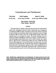
Higher bank credit-GDP ratios are a de…ning characteristic of greater domestic …nancial development.1 Moreover, economies di¤er widely in their domestic bank credit-GDP ratios. Economies also di¤er in the domestic external …nancing structure of …rms. Speci…cally, small and medium enterprises (SMEs) face relatively high barriers to access formal external …nancing from banks compared to large …rms, and therefore depend relatively more on informal external …nance in the form of inter…rm input credit. Inter…rm input credit is particularly prevalent in developing and emerging economies (DEMEs) relative to advanced economies (AEs) (see, for example, Chavis, Klapper and Love, 2011; Global Financial Development Report, henceforth GFDR, 2014; OECD, 2012, and Presbitero and Rabellotti, 2016, for Latin America; among others).2 Amid this backdrop, it is important to note that SMEs account for large shares of total aggregate employment and employment creation, particularly in the case of DEMEs (Ayyagari, Asli Demirgüç-Kunt, and Maksimovic, 2014). Within this context, an important question immediately follows: Does domestic …nancial development have implications for labor-market dynamics and, if so, why? The answer to the …rst part of our research question is given by a novel and robust stylized fact, which we document in Figure 1: The existence of a negative correlation between …nancial development and aggregate unemployment volatility in DEMEs, but a positive correlation between these 1
This is the de…nition of …nancial development that we adhere to. Our work does not address issues of …nancial integration between economies, but rather domestic …nancial development centered on …rm credit. Henceforth, we use the terms …nancial development, …nancial or credit deepening, and improved credit access interchangeably. 2 Small …rms in DEMEs rank access to formal credit as one of their most important operational obstacles. In fact, the share of total bank credit devoted to SMEs is only 20 percent in Latin America and developing Asia, whereas this share easily surpasses 40 percent in AEs (IMF, 2014; OECD, 2015). Moreover, compared to DEMEs, AEs tend to have higher shares of bank credit to the private sector as a percent of GDP.
2
variables in AEs. This relationship is statistically signi…cant for DEMEs, but statistically insigni…cant for AEs. DEMEs
Unemployment Volatility .1
.05
.05
.1
Unemployment Volatility .15
.2
.15
.25
AEs
50 100 150 Bank Credit to Private Sector Percent of GDP
20 40 60 80 100 Bank Credit to Private Sector Percent of GDP
Figure 1: Relationship between unemployment volatility and bank credit to the private sector as a percent of GDP. Red line: OLS regression of a country’s average unemployment volatility on a country’s average bank credit to the private sector as a percent of GDP. This regression yields: for DEMEs, a slope coe¢ cient signi…cant at the 5-percent level; for AEs, a slope coe¢ cient that is insigni…cant. Unemployment data are at yearly (time span varies across countries: earliest observation corresponds to 1950 and latest observation corresponds to 2015) frequency and HP-…ltered with a smoothing parameter equal to 6.25. Unemployment data are from the International Labour Organization and the OECD. Data on credit are from International Monetary Fund, International Financial Statistics and data …les, and World Bank and OECD GDP estimates.3 Countries are sorted into advanced economies (AEs) and developing and emerging economies (DEMEs) per the International Monetary Fund’s classi…cation.
Importantly, these relationships hold even after controlling for additional relevant variables that could in‡uence unemployment volatility across countries, including a host of labormarket regulation measures pertaining to hiring and …ring as well as productivity.4 More3
Unemployment data are from the International Labour Organization for: Albania, Algeria, Argentina, Bahamas, Barbados, Belize, Bulgaria, Chile, China, Colombia, Costa Rica, Ecuador, Honduras, Hong Kong, Indonesia, Israel, Jamaica, Korea, Luxembourga, Macau, Malaysia, Malta, Mauritius, Mexico, Morocco, Nicaragua, Pakistan, Panama, Paraguay, Philippines, Romania, Singapore, Sri Lanka, Syian Arab Republic, Thailand, Trinidad and Tobago, Uruguay, and Venezuela. Unemployment Data are from the OECD for Australia, Austria, Belgium, Canada, Czech Republic, Denmark, Estonia, Finland, France, Germany, Greece, Hungary, Iceland, Ireland, Italy, Japan, Netherlands, New Zealand, Norway, Poland, Portugal, Russia, Slovak Republic, Spain, Sweden, Switzerland, Turkey, United Kingdom, and United States. 4 These labor-market regulation indicators are obtained from the World Bank’s Doing Business Report
3
over, the relationship between GDP per capita, which is a standard measure of economic development, and unemployment volatility is insigni…cant for both DEMEs and AEs. To answer the second part of our research question, and motivated by our answer to the …rst part, we use a theoretical approach to shed light on economic fundamentals that may explain the link, or lack thereof, between domestic …nancial development and unemployment volatility across countries. We develop a small open economy real business cycle model with …nancial frictions, inter…rm input-credit, labor search, and heterogeneous …rms that, as a benchmark, captures key structural characteristics of DEME labor and credit markets. Guiding our analysis is the well-known fact that more …nancially-developed economies tend to have higher shares of bank credit devoted to SMEs compared to DEMEs (see Table A3 in the Appendix). Amid this backdrop, larger …rms on a stronger …nancial footing and with greater formal credit access extend inter…rm input credit— by de…nition, a form of informal external …nance— to SMEs.5 Indeed, an extensive theoretical and empirical literature stresses the role of inter…rm input credit as a key source of external …nancing for SMEs (see, for instance, McMillan and Woodru¤, 1999, Demirgüç-Kunt and Maksimovic, 2001, Fisman and Love, 2003, Allen et al. 2007, Beck et al., 2008, Hyndman and Serio, 2010, and GFDR, 2014).6 The importance of input credit for SMEs in select DEMEs is noted in (2014) and include: minimum wage for a full-time worker; the ratio of the minimum wage per value added per worker; the notice period for redundancy dismissal, and severance pay for redundance dismissal. 5 See García-Teruel and Martínez-Solano (2010); Garcia-Appendini and Montoriol-Garriga (2013); CarbóValverde, Rodríguez-Fernández, and Udell (2016); and Shenoy and Williams (2017). For example, extending trade credit allows …rms to expand their customer base, to operate in a competitive environment, and also to establish alternative insurance mechanisms against shocks. We do not model any speci…c microeconomic rationales for extending trade credit and instead focus on the implications of extending inter…rm input credit. 6 See Cuñat and Garcia-Appendini (2012) for an in-depth discussion of trade credit. Petersen and Rajan (1997) argue that small …rms, which often face credit constraints and limited access to formal …nancing, rely on suppliers to external resources. These suppliers are generally able to better monitor their customers’ activities relative to banks (Jain, 2001; Burkart and Ellingsen, 2004). Burkart and Ellingsen (2004), Daripa and Nilsen (2011), and Burkart, Ellingsen, and Giannetti (2011) provide theoretical rationales behind the use of trade credit. Pavón (2010) documents that input suppliers are the most important source of external
4
Table 1. Table 1: Input and bank credit among SMEs for select economies Country Input Credit Bank Credit (% of External Financing) (% of External Financing) Argentina 73:1 17:7 Brazil 45:2 39:9 Chile 62:7 32:5 Colombia 62:9 23:1 Mexico 62:7 17:6 Peru 40:5 42:1 Venezuela 59:2 28:9 Average 58:0 28:8 Notes: Source are author’s calculations using data from OECD (2013, Table 3.A1). Input credit is given by credit-based purchases from suppliers and advances from customers. Other sources of external …nancing, which are second-order to trade credit and bank credit, correspond to external …nancing from non-bank …nancial institutions and from moneylenders, friends, and relatives. Finkelstein Shapiro and González Gómez (2017) present similar evidence.
Importantly, as shown by Figure 2 for a broader set of DEMEs, the share of alternative …nancing sources— of which input credit is the most important— in total external …nancing is inversely related to the share of bank credit in total external …nancing. Of note, relationship is statistically signi…cant and it does not hold by construction as …rms can, in principle, tap into non-bank credit market …nance as well.7 …nancing for small …rms in Mexico, accounting for almost 70 percent of total external …nancing. This share is decreasing in …rm size, with commercial banks being comparatively more relevant among larger …rms. In other developing and emerging economies (DEMEs) roughly 60 percent of total external …nance comes from trade credit (Table A5 in the Appendix). As the Appendix shows in more detail, similar evidence holds in other DEMEs, where more than 50 percent of small-…rm entrepreneurs cite increased search for input suppliers to obtain external …nance support (see Tables A1, A2, A3, and A5 in the Appendix; IDB, 2005; GFDR, 2014). Furthermore, in-kind-based trade credit relationships are more likely to take place in economies with weaker institutional quality (Burkart and Ellingsen, 2004). Of note, trade credit is, by nature, relationship-based as opposed to spot-market-based. In fact, survey-based evidence con…rms SMEs’ search e¤orts to …nd supplier-based, non-bank external …nancing (Table A1 in the Appendix). Finkelstein Shapiro and González Gómez (2017) discuss the relevance of input credit and supplier relationships in detail as well. 7 Of note, recent studies have shown that some …rms resort to self-…nancing in order to overcome limited access to external …nancing. At the same time, …rms’…nancing patterns evolve as …rms age (see, for example, Midrigan and Xu, 2014). Shourideh and Zetlin-Jones (2016) document that, in contrast with publicly-traded …rms who primarily …nance the bulk of their investment internally, privately-held …rms …nance most of their investment using external …nancing. Publicly-traded …rms represent a minuscule share of …rms in DEMEs as most …rms in DEMEs tend to be small (GFDR, 2014). As such, our work focuses only on privately-traded
5
Alternative financing (% of external financing) .2 .4 .6 .8 0
0
.2 .4 .6 Bank financing (% of external financing)
.8
Figure 2: Alternative …nancing sources versus bank credit, both as a percent of total external …nancing. Data source: Allen, Carletti, Quianc, and Valenzuela (2012). Red line: OLS regression of alternative …nancing (as a percent of total external …nancing) on bank …nancing (as a percent of total external …nancing). This regression yields a slope coe¢ cient that is signi…cant at the 1-percent level.8
Our framework successfully replicates key labor market and business cycle properties of a representative DEME with quality labor market data: Mexico. We capture the relative importance of input credit among SMEs noted earlier by assuming two …rm categories— labeled “large”and “small.”While both …rm categories use labor (hired via frictional markets) and internally-accumulated capital to produce, we assume that small …rms also rely on capital supplied by large …rms via input credit. This assumption embodies the relative reliance of small …rms on informal external …nance vis-à-vis large …rms documented in the literature on input credit. Given our focus on …nancial development, our notion of small …rms is not related to size or age per se, but instead to the di¤erential external …nancing sources and …rms who, as suggested by existing evidence, do rely on (bank- and non-bank-based) external …nancing to operate. In addition, given our focus on business cycles and di¤erences across countries and not on …rms’life cycle patterns, we follow the literature on labor search frictions and business cycle dynamics and abstract from …rm-age considerations. 8 Country sample: Algeria, Argentina, Bangladesh, Belaruz, Brazil, Bulgaria, Chile, China, Colombia, Croatia, Ecuador, Egypt, Hungary, India, Indonesia, Kazakhstan, South Korea, Malaysia, Mexico, Morocco, Pakistan, Peru, Philippines, Poland, Romania, Russian Federation, South Africa, Syrian Arab Republic, Thailand, Turkey, Ukrain, Venezuela, and Vietnam. These countries fall into the DEME category per the International Monetary Fund’s classi…cation.
6
the degree to which certain …rms are less constrained in their access to bank credit. Our model analysis of the impact of …nancial development on labor market dynamics suggests that unemployment volatility is decreasing in the borrowing capacity of small and/or large …rms as long as input credit is su¢ ciently prominent in small-…rm production amid business cycle ‡uctuations driven by productivity and borrowing …nancial shocks. Intuitively, an improvement in …rms’borrowing capacity boosts the accumulation of capital, which makes …rms more resilient to credit disruptions and stabilizes the demand for input credit. These dynamics make vacancy postings and therefore unemployment less volatile for any given set of shocks. This mechanism is always at play, regardless of the degree of input credit in an economy. However, we show that the greater the degree of input credit in an economy, the greater the explicit linkages between large and small …rms. In fact, for a su¢ ciently low degree of input credit the relationship between …nancial development and unemployment volatility is for all purposes mute. These results are consistent with the relative importance of inter…rm input credit in DEMEs versus AEs. Therefore, our work puts forth the importance of input credit as a novel and key ampli…cation channel by which …nancial development can lead to lower unemployment volatility. The international business cycle literature has emphasized the role of interest rate shocks for business cycles in DEMEs (Neumeyer and Perri, 2005; Li, 2011; Chang and Fernández, 2013; Boz, Durdu, and Li, 2015). Recent literature has incorporated …nancial frictions (e.g., Kiyotaki and Moore, 1997; Jermann and Quadrini, 2012; Buera, Fattal-Jaef, and Shi, 2014; Iacoviello, 2015) into settings with frictional labor markets in a DEME context (Lama and Urrutia, 2011; Fernández and Herreño, 2012; Finkelstein Shapiro and González Gómez, 2017). In turn, a number of studies have explored the empirical connection between …nancial 7
development, growth, and aggregate volatility (Beck, Demirgüç-Kunt, Laeven, and Levine, 2004; Beck, Lundberg, and Majnoni, 2006; Aghion, Bacchetta, Rancière, and Rogo¤, 2009; Manganelli and Popov, 2012; Wang and Wen, 2013), and also between …nancial development and …rm dynamics (Arellano, Bai, and Zhang, 2012). While certain studies have explored the importance of sectoral heterogeneity (Beck, Demirgüç-Kunt, Laeven, and Levine, 2004; Manganelli and Popov, 2012; Dabla-Norris, Ji, Townsend, and Unsal, 2015), few, if any, have considered the implications for labor market dynamics. Relative to existing literature, to the best of our knowledge our paper is the …rst to: highlight a robust stylized fact explicitly linking …nancial development to cyclical labor market dynamics; and to stress the importance of …rms’external …nancing structure along with …rm heterogeneity in access to credit towards understanding a link between …nancial development and unemployment volatility. The remainder of this paper is organized as follows. Section 2 develops the model. Section 3 describes the model’s operationalization and main results. Section 4 concludes.
2
The Model
Our model is directly related to Epstein and Finkelstein Shapiro (2017) with regards to production, reliance on input-credit by a set of …rms, and the labor market, and Epstein, Finkelstein Shapiro, and González Gómez (2017) with regards to …nancial frictions and collateral constraints in a context of production heterogeneity. In turn, this last paper builds on Jermann and Quadrini (2012) and Iacoviello (2015).
8
2.1
Domestic Financial Intermediaries
In order to analyze the relevance of …rm heterogeneity amid …nancial development, both small (household) …rms and large …rms must face collateral constraints and are therefore considered borrowers. As such, domestic …nancial intermediaries— or banks— can e¤ectively be seen as suppliers of external funds to borrower …rms. We assume that …nancial intermediaries have a unit mass and are a distinct agent that chooses large- and small-…rm loan amounts ll;t and ls;t , respectively, and consumption cb;t to maximize E0 cb;t = Rt 1 lt is
b
1
t t=0 b u(cb;t )
subject to the constraints
lt , where: lt = ll;t + ls;t ; and u0 > 0; u00 < 0. The subjective discount factor
2 (0; 1) and Rt is the gross lending rate for large and small …rms.9 The …rst-order
conditions yield u0 (cb;t ) =
2.2
P1
b Et u
0
(cb;t+1 )Rt .
Large Firm Entrepreneurs
We assume that large …rms can choose how much of their internally-accumulated capital stock to use in their own production and how much of this capital to rent out to small …rms— our notion of input-credit.10 Large-…rm entrepreneurs have a unit mass and choose consumption cl;t , desired employment (denoted nl;t+1 from the demand side perspective) vacancies vl;t , capital kl;t+1 , the fraction of existing capital to be used within the …rm ! t , and borrowed funds ll;t to maximize E0
P1
t=0
t l u(cl;t )
(where u0 < 0 and u00 < 0) subject to: the resource
9 The Appendix discusses the results from introducing costly …nancial intermediation, which generates an explicit spread between lending and deposit rates based on Cúrdia and Woodford (2010), as well as higher lending rates for small …rms relative to large …rms. Our results remain the same if we characterize …nancial development by a joint improvement in borrowing capacity and a reduction in both intermediation costs and interest rate spreads. 10 See, for example, Finkelstein Shapiro (2014) and Epstein and Finkelstein Shapiro (2017) for richer speci…cations with frictional input credit markets.
9
constraint
cl;t = pl;t yl;t
wl;t nl;t
(vl;t ) o
+ (rs;t +
il;t + ll;t
Rt 1 ll;t
1
! t )kl;t ,
) (1
where pl;t is the price of output, yl;t is output (yl;t = zl;t F(nl;t ; ! t kl;t ), F is constant returns to scale, and zl;t is exogenous sectoral productivity), wl;t is the wage, vl;t are vacancies that are posted at a cost
0
(vl;t ) with
> 0 and
00
> 0, il;t is investment, and rs;t is
the input-credit capital rental rate; standard laws of motion for employment and capital, nl;t+1 = (1
l
l
) (nl;t + vl;t ql;t ) (where
is the exogenous job-destruction probability and
ql;t is the endogenous job …lling probability), and kl;t+1 = (1
)kl;t + il;t (where
depreciation rate of capital), respectively; a collateral constraint Rt ll;t + wl;t nl;t
is the l;t kl;t+1 .
Note that in equilibrium, the measure of small …rm owners os;t must be equal to the supply of unused capital by large …rms, (1
! t )kl;t . Moreover, we assume that any depreciated
input-credit capital net of the exogenous depreciation of input credit other than physicalcapital depreciation (
o
)(1
o
is covered by large …rms. This assumption is captured by the term
! t )kl;t .
The sectoral collateral constraint follows Quadrini (2012) and Iacoviello (2015).11 And, following this literature we assume that holds with equality. Also, note that equal a larger value of
l;t
12
b,
<
which guarantees that the constraint
determines the …rm’s borrowing capacity: all else
is consistent with the …rm’s existing capital being worth more
as collateral.12 (We assume that 11
l;t
l
l;t
has mean
l
and follows a stochastic process, and the
For a two-sector application, see Epstein, Finkelstein Shapiro, and González Gómez (2017). The collateral constraint assumes that the …rm must …nance the entirety of the wage bill, which is
10
…rm’s total wage bill must be paid in advance— see, for instance, Neumeyer and Perri, 2005; Iacoviello, 2015). Large-…rm optimization yields the following 4 equations. First, the large-…rm Euler equation 1
where:
l;t
l;t l;t
= Et
l t+1jt
(pl;t+1 zl;t+1 F!kl ;t+1 ) + (1
),
is the (collateral) multiplier on the large …rm’s borrowing constraint normalized
by the marginal utility of large-…rm consumption; and
l t+1jt
lu
0
(cl;t+1 )=u0 (cl;t ) is the large
…rm’s stochastic discount factor. Intuitively, the marginal cost of accumulating capital (the left-hand side of this equation, which is decreasing in the collateral multiplier and borrowing capacity) is optimally set equal to the marginal bene…t (the right hand side of this equation, which is increasing in the stochastic discount factor and the marginal revenue product of capital, but decreasing in the capital depreciation rate). Second, the large-…rm job creation condition
0
(vl;t ) = (1 ql;t
l
)Et
l t+1jt
pl;t+1 zl;t+1 Fnl ;t+1
wl;t+1 [1 +
l;t+1 ]
+
0
(vl;t+1 ) ql;t+1
,
which equates the expected marginal cost of posting an additional vacancy (which is equal to the marginal cost of a posting a vacancy per the expected duration of the position being vacant) to the expected bene…t of …lling an open vacancy with an additional worker (which is increasing in the stochastic discount factor, the marginal revenue product of labor, and the continuation value of a match, but decreasing in a worker’s wage adjusted for the collateral standard in related literature— assuming that only a fraction of the wage bill needs to be …nanced does not change our main results. A similar comment applies to small …rms below.
11
multiplier as a re‡ection of the fact that the …rm must …nance the wage bill, and also decreasing in the exogenous separation probability). Third, the large-…rm input-credit supply condition
pl;t zl;t F!kl ;t = rs;t + (
o
),
which equates the marginal cost of devoting a unit of capital to a small …rm (which is equal to the marginal revenue product of capital) to the marginal bene…t (the rental rate and the value of a depreciated unit of capital). Fourth, an optimal borrowing condition, 1
Rt
l;t
= Et
l t+1jt Rt ,
which equates the mar-
ginal bene…t from borrowing funds (which is decreasing in the gross lending rate and the collateral multiplier) to the expected discounted gross rate on borrowed funds (see, for instance, Iacoviello, 2015). Rearranging this last equation to yield 1=Rt
l;t
= Et
l t+1jt
it
follows that a rise in the gross lending rate or an increase in the collateral multiplier both put downward pressure on the large-…rm’s stochastic discount factor.
2.3
Small Firms and Households
Following a frictionless input-credit version of Epstein and Finkelstein Shapiro (2017), we assume that each small …rm uses one and only one unit of input-credit capital to produce (assuming variable input-credit utilization within a given …rm does not change our results).13 Even though small …rms can accumulate capital internally, a prerequisite for the existence of a small …rm (and therefore, a small-…rm owner) is that it relies on input-credit as an input 13
We note that modeling input-credit relationships via capital search, as in Finkelstein Shapiro (2014) and Epstein and Finkelstein Shapiro (2017), does not change any of our conclusions.
12
supplied by a large …rm. Also, as shown below, household members can be engaged in 4 economic activities: (1) employed in a small …rm; (2) employed in a large …rm; (3) being a small …rm owner; (4) or unemployed. There is no labor force participation margin and the labor force is normalized to one. Similar to Epstein and Finkelstein Shapiro (2017), total pro…ts for small …rms are
s;t
= [ps;t zs;t F (ns;t ; ks;t ; os;t ) rs;t os;t
(vs;t )os;t + ls;t
ws;t ns;t
is;t ]
Rt 1 ls;t 1 ,
where: ps;t is the price of output; ys;t is output (ys;t = zs;t F (ns;t ; ks;t ; os;t ), F is constantreturns-to-scale, and zs;t is exogenous sectoral productivity); ns;t is the measure of small-…rm salaried workers from the demand-side perspective (Epstein and Finkelstein Shapiro, 2017); ks;t is the internally-accumulated capital stock; is;t denotes total small …rm investment in capital ks;t ; os;t is the measure of small …rm owners (given our assumption of one unit of input credit per small …rm, os;t is also the measure of input-credit capital); ws;t is the wage; rs;t is the input-credit-capital rental rate; the cost of vacancy creation per small …rm owner is (vs;t ) with
0
> 0 and
00
> 0; and small …rms borrow external funds ls;t at a gross interest
rate R.14 Households have a unit mass and own small …rms and make decisions for these …rms from an input-demand perspective. Note that we allow households to hold foreign debt to follow the literature on DEME business cycles. Importantly, given that households account for the 14
Given that os;t is the measure of small …rm owners and all …rms have the same exogenous productivity and a constant-returns production technology, dividing s;t by os;t yields pro…ts per small …rm.
13
bulk of total consumption in the model, this assumption gives households an instrument to smooth consumption. At the same time, the presence of collateral constraints implies that the lending rate and foreign interest rate will di¤er as a result of a positive multiplier on the collateral constraint. This can be rationalized as follows: the positive collateral constraint multiplier may embody other factors (di¤erential access to credit markets, intermediation costs that may di¤er between …rms and individuals, etc.) which we do not explicitly model and that imply a discrepancy between the cost of borrowing for …rms and the cost of accessing foreign assets by households.15 Households choose consumption ch;t , foreign debt bt , desired demand for small-…rm workers ns;t+1 , the desired measure of small …rm owners os;t+1 , resources devoted towards establishing small …rms st , internal capital ks;t+1 , vacancies vs;t , and borrowed funds ls;t from domestic …nancial intermediaries to maximize E0 to the budget constraint16
ch;t + (st ) + Rt 1 bt
a law of motion for capital ks;t+1 = (1 labor input ns;t+1 = (1 (1
o
ws;t ns;t
s
1
=
s;t
+
P1
t h u(ch;t )
t=0
t
(u0 > 0 and u00 < 0) subject
+ ws;t nss;t + wl;t nsl;t + bt ,
)ks;t +is;t , the perceived law of motion for small-…rm
) (ns;t + os;t vs;t qs;t ), the evolution of small …rm owners os;t+1 =
) (os;t + Mk st ), where Mk is scaling parameter, and a borrowing constraint Rt ls;t – s;t ks;t+1 ,
where (st ) is a resource cost with
receive income from …nal-goods …rm pro…ts, 15
t,
0
(st ) > 0 and
00
(st ) > 0; households
large- and small-…rm workers, wl;t nsl;t and
Of note, abstracting from foreign debt (which would imply a closed economy) does not change any of our conclusions. 16 As such, households can be seen as hiring small-…rm workers for their …rms by posting vacancies to attract unemployed members from households other than their own.
14
ws;t nss;t , and take these pro…ts and wages as given— -nsl and nss denote sectoral employment from the supply-side perspective and in the absence of labor force participation decisions, nsl and nss are taken as given by the household; Rt is the gross foreign interest rate on foreign debt and Rt = R +
b
[exp(bt
b)
1] with
b
> 0 and steady-states R and b
(Schmitt-Grohé and Uribe, 2003); qs;t is the endogenous job-…lling probability; and workers are separated from small …rms with exogenous probability
s
…rm’s borrowing capacity (all else equal a larger value of
s;t
. Finally,
s;t
determines the
is consistent with the small
…rm’s existing capital being worth more as collateral). Small-…rm and household optimization yield the following 5 conditions. First, a standard Euler equation for foreign debt, 1=Rt = Et
h t+1jt ,
where:
h t+1jt
hu
0
(ch;t+1 )=u0 (ch;t ) is the
household’s stochastic discount factor. Second, an input-credit demand condition
0
(st ) = (1
o
)Et
h t+1jt
f[ps;t+1 zs;t+1 Fos ;t+1
ro;t+1
(vs;t+1 )] +
0
(st+1 )g ,
where the marginal cost of getting input credit (or, equivalently, having an additional small …rm owner) is equal to the expected marginal bene…t of doing so. This is akin to a standard capital Euler equation, but in our case with regards to input credit (i.e. small …rm owners given our assumption of one unit of input credit per small …rm). Third, a job creation condition
0
where:
(vs;t ) = (1 qs;t
s;t
s
)Et
h t+1jt
ps;t+1 zs;t+1 Fns ;t+1
ws;t+1 [1 +
s;t+1 ] +
0
(vs;t+1 ) qs;t+1
.
is the multiplier on the small …rm’s borrowing constraint normalized by the
15
marginal utility of small-…rm consumption. Fourth, a standard internal-capital accumulation condition, 1
s;t s;t
= Et
h t+1jt
fps;t+1 zs;t+1 Fks ;t+1 + (1
And …fth, an optimal borrowing condition, 1
Rt
s;t
= Et
)g .
h t+1jt Rt .
The interpretation of
these last 3 equations is entirely akin to their large-…rm counterparts.
2.4
Closing the Model
De…ne unemployment as ut
1 –nl;t –ns;t –os;t . The functions ml;t = ml (vl; ,ut ) and ms;t
= ms (vs;t os;t ,ut ) are standard constant returns to scale matching functions. The job-…nding probabilities are fj;t = mj;t =ut and for j 2 fl; sg. In turn, the job-…lling probabilities are qs;t = ms;t =(vs;t os;t ) and ql;t = ml;t =vl;t . Labor market tightness in each sector is and
l;t
(vs;t os;t )=ut
s;t
vl;t =ut . All salaried job-…nding probabilities are increasing in labor tightness.
Wages are determined via Nash bargaining. Due to di¤erences in the discount factors between households and …rms and the timing of the matching processes, no closed-form solution for wages can be obtained. For expositional briefness, the relevant value functions and Nash bargaining problems that implicitly de…ne these prices are presented in the Appendix.17 Total output aggregates large- and small-…rm output using the constant elasticity of substitution (CES) function yt = y(yl;t ; ys;t ). Final goods …rms maximize pro…ts 17
t
= [y(yl;t ; ys;t )
The Appendix also presents implicit expressions for wl and ws that show how wages are in‡uenced by (1) formal credit market conditions (embodied in l and s via …rms’ discount factors), (2) marginal productivities, and (3) sectoral market tightness in their own employment category and in other categories. Of note, volatility in credit conditions in‡uences how …rms value future employment relationships, which a¤ects hiring decisions. Also, the hiring decisions of …rms in a given sector have spillover e¤ects on the decisions of …rms (and households) in other sectors by a¤ecting employment outside options (i.e., sectoral market tightness). Therefore, as …nancial development takes place, the variability of salaried labor and credit market conditions due to productivity and …nancial disturbances changes.
16
– pl;t yl;t – ps;t ys;t ], where the price of …nal output is normalized to 1. We obtain standard relative prices for large and small …rm output, pl;t = yyl (yl;t ; ys;t ) and ps;t = yys (yl;t ; ys;t ), respectively. Finally, the aggregate resource constraint is
yt = ct + il;t + is;t + (st ) + (vl;t ) + (vs;t )os;t + tbt ,
where: ct = ch;t + cl;t + cb;t is total consumption; and the trade balance is de…ned as tbt
Rt 1 bt
3
1
–bt .
Operationalization and Results
3.1
Operationalization
We assume that ln zj;t = (1
%z ) ln(zj ) + %z ln zj;t
speci…c parameter, %z 2 (0; 1), and "zt
N (0;
2 z)
1
+ "zt for j 2 fl,sg, where zj is a sector-
denotes the aggregate productivity shock.
Similarly, sectoral borrowing capacity follows an AR(1) process with a common …nancial shock: ln
j;t
= (1
% ) ln( j ) + % ln
parameter, % j 2 (0; 1), and "t
N (0;
j;t 1 2
+ "t for j 2 fl; sg, where
j
is a sector-speci…c
).
A time period is 1 quarter. Table 2 summarizes the functional forms we use. Note that although not stated in the model description for expositional simplicity, following related literature, we introduce standard capital adjustment costs
(kj;t ; kj;t+1 ).
Also, as shown in Table 2, in the functional form for F (ns;t ; ks;t ; os;t ),
k
determines
the relative importance of capital obtained via input credit in the production function of 17
small …rms. Intuitively,
k
and the ease with which …rms can access …nancial credit may
be endogenously related, for instance, if greater …nancial credit pushes small …rms to reduce their dependence on input credit. However, we remain purposefully agnostic about this potentially endogenous relationship, since this approach allows us to carefully dissect the importance of each of the model’s ingredients in a disciplined and transparent way. Recall that our objective is not to explain the external …nancing structure of …rms, but rather to shed light on the implications for labor-market dynamics of …rms’existing external …nancing structure.
Variable yt
Table 2: Functional forms Functional Form h i1 a a y + (1 ) y s;t a l;t a a 2 (0; 1) and
F (ns;t ; ks;t ; os;t ) (ns;t )1 s (os;t ) k (ks;t )1 F(nl;t ; ! t kl;t ) (nl;t )1 l (! t kl;t ) l ml;t Ml (ut ) (vl;t )1 ms;t (kj;t ; kj;t+1 ) (st ) (vj;t ) u(cj )
s
c1j
= (1
a
1
2 (0; 1) l 2 (0; 1) Ml is match scaling and is match elasticity Ms is match scaling and is match elasticity for j2 fl;sg; standard in related literature k ; k > 0; Merz and Yashiv (2007) j ; v > 0 for j2 fl;sg; standard in related literature > 0 for j2 fl;sg; j standard in related literature s
Ms (ut ) (vs;t os;t )1 1)2 kj;t
('k =2) (kj;t+1 =kj;t k k (st ) v j (vj;t )
Notes
)
Table 3 summarizes the parameter values we adopt. A standard assumption in models with collateral constraints is that
b
>
h;
l
(see, for instance, Iacoviello, 2015), which
we implement, so that …rms’ collateral constraints are always binding.18 Of course, while empirically …rms may not always face binding …nancing constraints over the business cycle, our main objective is to explore the cyclical unemployment implications of improving …rms’ 18
We experiment and …nd that our conclusions do not hinge on other plausible values for
18
b,
h,
and
l.
access to credit relative to a baseline, more constrained economy. As such, our quantitative analysis abstracts from occasionally binding constraints as these are not central to our focus.19 Table 3: Parameter Assumptions Parameter Value Notes 0:320 Epstein and Finkelstein Shapiro (2017) l 0:270 Epstein and Finkelstein Shapiro (2017) s 0:985 Binding collateral constraint; Iacoviello (2015) b 0:885 Binding collateral constraint; Iacoviello (2015) h 0:885 Binding collateral constraint; Iacoviello (2015) l 0:025 Standard in related literature 2:000 j 2 fl; s; og; Merz and Yashiv (2007)20 j 0:500 Petrongolo and Pissarides (2001)21 0:700 Benchmark; Epstein and Finkelstein Shapiro (2017)22 a l 0:030 Bosch and Maloney (2008) s 0:070 Bosch and Maloney (2008) o 0:040 Bosch and Maloney (2008) %z 0:950 Aguiar and Gopinath (2007) 2:000 Standard in related literature zs 1:000 Normalization; see Appendix for details zl 2:219 Busso, Fazio, and Levy (2012); see Appendix for details Table 4 summarizes the calibrated parameters used in our benchmark simulation. We use Mexico as a reference DEME given its rich labor market data. We note that
s
>
l
may
initially seem at odds with the well-known severity of …nancing constraints among small …rms. However, we stress that …rms also di¤er in their steady-state levels of internallyaccumulated capital. In particular, small …rms have less capital and it is the total borrowing 19
Of note, a related segment of the literature on …nancial frictions focuses on the misallocation and totalfactor-productivity implications of these constraints as part of the development process (see Buera, Kaboski, and Shin, 2011; Buera, Fattal-Jaef, and Shi, 2014; among others). Since our focus is not on misallocation or micro-level di¤erences in …rm productivity, we stay close to well-known studies on business cycles and …nancial frictions. 20 Our value implies that the total resource cost from vacancy posting in the benchmark calibration is around 1 percent of output, in line with the literature (Boz, Durdu, and Li, 2015). 21 In line with related literature, the bargaining power of all types of workers is = 0:5. Our conclusions do not change if we assume that and/or di¤er at the sectoral level. 22 This value implies a relatively high degree of imperfect substitutability between sectoral
output (other reasonable values, whether higher or lower, do not change our conclusions). 19
capacity,
l kl
for large …rms and
s ks
for small …rms, that ultimately matters for the relative
sensitivity of …rms to shocks. Indeed, controlling for …rms’di¤erential internal capital levels, the total borrowing capacity of large …rms is much higher than the one for small …rms. That is, in the steady state,
l kl
>
s ks .
Thus, the calibrated values for
l
and
s
are consistent
with large …rms having better access to formal …nancing relative to small …rms as suggested by existing empirical evidence. Regarding employment shares, according to Mexico’s National Survey on Urban Employment and National Survey on Occupation and Employment, the share of self-employment in Mexico is close to 23 percent (a lower bound). Around 30 percent of those self-employed work in …rms with more than one worker (that is, in salaried …rms). Hence the share of small …rm owners we use in our benchmark calibration. In the model, the self-employed are accounted for in the share of workers in small …rms since, similar to small-…rm salaried workers, selfemployment is countercyclical. Also, as noted in Epstein and Finkelstein Shapiro (2017), the fact that Ms >Ml should not be taken as implying that large …rms are less e¢ cient at hiring than small …rms, but instead may re‡ect aspects of the economic environment that we are not explicitly modeling (institutional or regulatory factors that a¤ect the matching process, for example). Moreover, the values for these matching parameters imply higher job-…nding probabilities for small-…rm employment relative to large-…rm employment, which is consistent with evidence from Bosch and Maloney (2008) (where informal employment is mainly concentrated in small …rms).
20
Table 4: Calibrated Parameters Parameter Value Notes 0:291 Match Mexico empirical average domestic credit-to-GDP l ratio (=0.20; World Bank Development Indicators) 0:614 Match share of credit to small …rms in sample of DEMEs s (= 0.10; OECD, 2012) 0:650 Match Mexico distribution of capital stock across …rms k Busso, Fazio, and Levy (2012) for Mexico. b 0:673 Match Mexico (steady-state) foreign debt-to-GDP ratio (= 0.30; Aguiar and Gopinath, 2007) Ml 0:076 Match nl = 0:40 in Mexico (statistical agencies) Ms 0:448 Match ns = 0:48 in Mexico (statistical agencies) Mk 0:027 Match os = 0:07 in Mexico (statistical agencies) 0:034 Vacancy cost is 3.5 percent of sectoral wages (Levy, 2007) l 0:011 Vacancy cost is 3.5 percent of sectoral wages (Levy, 2007) s 0:320 Capital-search cost equals 3 months of sectoral wages k (McKenzie and Woodru¤, 2008) 0:341 Match (p l yl )=y=0:55 in Mexico (Busso, Fazio, and Levy, 2012 a , and Enterprise Surveys) 0:010 Stationary debt holdings without a¤ecting aggregate b dynamics (Schmitt-Grohé and Uribe, 2003) 'k 32:140 Match investment volatility relative to output in Mexico (1993:Q1-2007:Q4) 0:017 Match output volatility in Mexico (1993:Q1-2007:Q4) z % 0:900 Persistence of output in Mexico (1993:Q1-2007:Q4) 0:028 Cyclical correlation between output and wages in Mexico (1993:Q1-2007:Q4) Given the large number of state variables, global solution methods become highly intractable. Therefore, we log-linearize the model around the non-stochastic steady state and use a …rst-order approximation to the equilibrium conditions. The model is simulated for 2100 periods. The …rst 100 periods are discarded, and an HP …lter with smoothing parameter 1600 is applied to the remaining series.
21
3.2
Business Cycle Moments
Business cycle ‡uctuations in the benchmark model are driven by productivity and borrowing capacity (…nancial) shocks, only. Table 5 shows business cycle statistics for Mexico (“Data”) and compares them to results from our benchmark economy (“Model”). The model performs well in quantitatively capturing the cyclical properties of the data on all fronts, except the volatility of unemployment. Of note, the benchmark model: successfully generates standard deviations of consumption and wages higher than the standard deviation of output, which is a well-known feature of DEMEs (Boz, Durdu, and Li, 2015); generates a countercylical trade balance-output ratio;23 generates a factual autocorrelation of unemployment. and generates factual correlations with output of both large- and small-…rm employment.24 The limited ability to generate overall high unemployment volatility is a well-known and well-documented re‡ection of the “Shimer puzzle” (Shimer, 2005). Addressing this common limitation of search models lies outside the scope of our work as we are interested in di¤erences in unemployment volatility across di¤erent …nancial development equilibria. As such, not being able to exactly match the volatility of unemployment is of entirely second order for our purposes. 23
Removing the wage bill from …rms’ collateral constraints improves the countercyclicality of the trade balance-output ratio, but reduces the volatility of wages somewhat. However, it is still the case that both wages and consumption remain more volatile relative to output, as in the data. Results available upon request. 24 The majority of formal salaried workers are in large …rms and the majority of informal workers are in small …rms (Busso, Fazio, and Levy, 2012). This explains why, given our mapping between the data and the model, small …rm employment is countercyclical (for empirical evidence, see Bosch and Maloney, 2008; Fernández and Meza, 2015). Within the context of our model with formal …nancing, this mapping is an approximation as many small …rms (which are generally informal) may not have full access to formal …nancing, though this fact is re‡ected in the collateral constraint (adjusted for the level of capital) for small …rms. The mapping we use is not problematic since a share of small …rms do indeed have access to formal …nancing (World Bank Enterprise Surveys). As shown in Table 5, it is worth highlighting that the model is consistent with speci…c second moments of the labor market that we do not target, which adds considerable validity to our framework.
22
Table 5: Business Cycle Statistics, Data vs. Model A. Targeted moments Statistic (yt ; yt 1 ) yt i;t Data 2:390 6:644 0:750 Model 2:390 6:644 0:745 B. Non-targeted moments Statistic (nl;t ; yt ) (ns;t ; yt ) (ut ; yt ) (ut ; ut c;t w;t ut Data 3:011 4:701 20:66 0:740 0:470 0:780 0:840 Model 2:814 3:441 0:764 0:645 0:168 0:549 0:874
(wt ; yt ) 0:560 0:566 1)
(tbt =yt ; yt ) 0:750 0:333
Notes: x refers to the standard deviation of variable x. (x; y) refers to the correlation of x with y . All second moments for the model are obtained using …ltered series to make them comparable to the data. The empirical moments for large-…rm and small-…rm employment are based on data from Mexico’s employment survey (ENEU). The empirical volatility of consumption and wages, the cyclicality of unemployment, and the persistence of output and unemployment are from Boz, Durdu, and Li (2015).
3.3
Financial Development
In order to study the link between …nancial development and unemployment volatility, we focus on three parameters:
l
(the large …rm’s steady-state borrowing capacity);
…rm’s steady-state borrowing capacity); and
k
s
(the small
(which determines the relative importance
of matched capital obtained via input credit in the production function of small …rms).25 Recall that a higher
k
implies that, all else equal, small-…rm production is more intensive
in input credit; that is, small …rms rely relatively more on informal external …nance.26 Figure 3 plots the economy’s steady-state bank credit-GDP ratio and unemployment volatility for di¤erent combinations of
l
and
k
(top two panels) and of
s
and
k
(bottom
two panels), respectively.27 In each graph the benchmark calibration point is highlighted 25
See Dabla-Norris et al. (2015) for a related approach that studies …nancial development. Of note, as part of our robustness analysis below, we show that having di¤erences in borrowing capacity between large and small …rms (that is l 6= s as opposed to l = s = ), which re‡ect small …rms’ more constrained status relative to large …rms as in the data, is important for quantitatively explaining the link between …nancial development and unemployment volatility. 27 For consistency with Table 5, Figure 3 is generated using simulated data at quarterly frequency. We 26
23
with a white dot. Note that, all else equal, a higher borrowing capacity among large or small …rms (
l
or
s)
is associated with a higher steady-state bank credit-GDP ratio. In contrast,
all else equal a higher share of input-credit-capital in production ( k ) is associated with a lower steady-state bank credit-GDP ratio. Note from Figure 3 that the parameter combinations for
l,
s,
k
generate the range of
steady-state bank credit-GDP ratio that matches the empirical range of this variable as shown in Figure 1.
Figure 3: Impact of changes in key parameter values on the steady-state bank credit-GDP ratio and unemployment volatility (benchmark model).
Also, per Figure 3 unemployment volatility is decreasing under, all else equal, higher l
and, all else equal, higher
s,
but only at high values of
k
(i.e., when inter…rm input
credit is a relatively important component among small …rms, as is the case in DEMEs). For low values of
k,
improvements in …rms’ borrowing capacity have virtually no impact
note that the main results are qualitatively identical if we consider simulations at a yearly frequency.
24
on unemployment volatility, as is the case in AEs. So, unemployment volatility is always rising in
k,
decreasing in
but the rate at which unemployment volatility is decreasing in k:
l
and
s
is
Similarly, from the perspective of …nancial development re‡ected in …rms’
domestic external …nancing structure, unemployment volatility is rising in
k
(which itself is
negatively correlated with the steady-state bank credit-GDP ratio), but only for low levels of …rms’borrowing capacity
l
and
s.
Keeping Figure 3 in mind, recall from the facts in the Introduction that, all else equal, there exists a markedly negative and statistically signi…cant relationship between unemployment volatility and …nancial development in DEMEs, and a slightly positive though statistically insigni…cant relationship between …nancial development and unemployment volatility in AEs (even after controlling for other potential factors that may in‡uence the volatility of unemployment). Furthermore, recall that inter…rm input credit is a key characteristic of small …rms’external …nancing structure in DEMEs but plays a less signi…cant role in AEs, where …rms rely relatively more on more formal sources of external …nancing. All told, we conclude that the model can successfully generate both the factual negative relationship between domestic …nancial development and unemployment volatility in DEMEs and also the factual disconnect between domestic …nancial development and unemployment volatility in AEs documented in Figure 1. In doing so, the model suggests that the statistically signi…cant negative correlation between unemployment volatility and …nancial development observed in DEMEs can be traced back to increases in …rms’borrowing capacity occurring amid a high degree of input-credit relevance in production. In contrast, the statistically insigni…cant relationship between unemployment volatility and …nancial development observed in AEs can be traced back to increases in …rms’borrowing capacity occurring amid 25
a low degree of input-credit relevance in production. Of course, taken together these results suggest that an endogenous negative relationship between …nancial development and input-credit relevance in production (or, more broadly, …rms’external-…nancing structure) may exist, which is intuitive. However, as noted earlier, we have purposefully taken an agnostic modeling approach to pinpoint in a disciplined and transparent way the key features of an economy’s domestic …rm-external-…nancing structure that can rationalize the stylized facts observed in the empirical data.
3.4
Economic Mechanisms
Figure 4 sheds light on the driving forces behind our main results. This …gure shows: the volatility of large-…rm and small-…rm employment and wages (top 4 panels); the volatility of the share of large-…rm capital devoted as input credit to small …rms, ! (bottom left panel); and the volatility of unemployment (bottom right panel). (Similar patterns are observed for all of these variables when we change
l
and
k
the interpretation for which is entirely akin to
that stated further below— recall that changes in
l
and
s
have the same qualitative impact
on unemployment volatility; so, without loss of generality we focus on …nancial development equilibria based on changes in 4 is: decreasing in
k;
s
and
k .)
and decreasing in
l
The volatility of all variables depicted in Figure only at relatively high values of
26
k.
Figure 4: Impact of changes in key parameter values on: sectoral employment volatility; sectoral wage volatility; fraction of large-…rm capital devoted to input-credit volatility; unemployment volatility (benchmark model).
To understand the results shown in Figure 4, note that an improvement in small …rms’ borrowing capacity
s
amid productivity and …nancial shocks boosts the accumulation of
capital. This higher capital stock, all else equal, makes …rms more resilient to credit disruptions, in turn making vacancy postings less volatile for a given set of shocks. Therefore, small-…rm employment becomes more stable. Critically, this greater employment stability also stabilizes the demand for input credit, which leads to a fall in the volatility of !. All else equal, this fall in the volatility of ! stabilizes large …rms’pro…ts and vacancy postings and, as a result, large-…rm employment as well. So, both large-…rm and small-…rm employment, and ultimately aggregate unemployment, become less volatile amid …nancial development. This mechanism is always at play, regardless of the degree of input credit in an economy
27
(as captured by
k ).
However, the greater the degree of input credit in an economy, the
greater the explicit linkages between large and small …rms. Therefore, input credit is the key ampli…cation channel by which …nancial development can lead to lower unemployment volatility. Importantly, note that a reduction in unemployment volatility tied to …nancial development is not due to an increase in sectoral (and aggregate) real-wage volatility. In fact, as shown in Figure 4, both wage and unemployment volatility fall as a result of …nancial development. This result consistent with the evidence in Boz, Durdu, and Li (2015), who document that advanced economies have, on average, lower real wage volatility relative to emerging economies. In sum, our results suggest that both …nancial development as re‡ected in a higher aggregate bank credit share and …rms’domestic external …nancing structure— especially as it relates to the degree of dependency on inter…rm input-credit relationships among small …rms— are critical to shed light on the link between domestic …nancial development and unemployment volatility.
3.5
Nested Models and Robustness Analysis
In what follows, we present evidence that supports our framework and assumptions on heterogeneity across …rm categories in their …nancial structure and borrowing capacity by showing that simpler models either underperform in matching important facts compared to our benchmark speci…cation or fail to replicate the empirical relationship between …nancial development and unemployment volatility. In particular, we consider (1) a version of our model
28
with the same borrowing capacity parameter across …rm categories (that is, (“Model
l
=
s
l
=
s
= )
= ”); (2) a version of our model without input credit linkages (i.e., ! = 1
for all t) and therefore no small …rm owners os (“No ! and No os ”) (without loss of generality, we show the results under a change in hold under a change in
l );
s
for nested model (2), but the same results
and (3) a standard one-sector model with collateral constraints
(“One Sector Model”).28 All of these models are nested within our benchmark framework. First, Table 6 compares business cycle moments across models to our benchmark model. Second, Figures 5 and 6 plot equilibrium bank credit-GDP ratio and unemployment volatility for di¤erent
l,
s,
and
k,
(=
l
=
s)
and
k,
or , depending on whether nested model
(1), (2), or (3), respectively, is under consideration. For reference, the top panel of Figure 5 plots outcomes for the benchmark model. Table 6: Business Cycle Statistics, Data vs. Benchmark Model and Nested Models A. Targeted moments Statistic (yt ; yt 1 ) (wt ; yt ) yt i;t Data 2:390 6:644 0:750 0:560 Model 2:390 6:644 0:745 0:566 B. Non-targeted moments Statistic (n (ns;t ; yt ) (ut ; yt ) (ut ; ut 1 ) (tbt =yt ; yt ) c;t w;t ut l;t ; yt ) Data 3:011 4:701 20:66 0:740 0:470 0:780 0:840 0:750 Benchmark Model 2:814 3:441 0:764 0:645 0:168 0:549 0:874 0:333 Model l = s = 3:045 3:667 0:912 0:632 0:287 0:512 0:838 0:263 No ! and No os 1:768 3:868 1:196 0:426 0:025 0:132 0:486 0:658 One Sector Model 1:768 3:911 0:748 0:664 0:446 0:835 0:671 Notes: x refers to the standard deviation of variable x. (x; y) refers to the correlation of x with y . All second moments for the model are obtained using …ltered series to make them comparable to the data. The empirical moments for large-…rm and small-…rm employment are based on data from Mexico’s employment survey (ENEU). The empirical volatility of consumption and wages, the cyclicality of unemployment, and the persistence of output and unemployment are from Boz, Durdu, and Li (2015). 28
Nested model (2) is a simple two-sector model where the only di¤erences between “small” and “large” …rms are di¤erences in exogenous sectoral productivity and steady-state borrowing capacity. Both …rm categories have the same production technology (with internally-accumulated capital and labor as inputs).
29
Per Table 6, the model under identical borrowing capacity parameters across …rm categories does well in replicating key second moments but, importantly, as shown in the bottom panel of Figure 5, this model cannot generate the relationships between …nancial development and unemployment volatility observed in the data. In fact, counter to the data, unemployment volatility is actually rising in borrowing capacity regardless of the level of k .
Figure 5: Impact of changes in key parameter values on the steady-state bank credit-GDP ratio and unemployment volatility (benchmark model and alternative model with common borrowing capacity).
This counterfactual result is also observed in Figure 6 resulting from the one-sector model and the model that abstracts from input credit. As shown in Table 6, these models also perform worse in matching key second moments for Mexico compared to the benchmark model. (Note that Figure 6 presents results in 2 dimensions only since the models presented in this …gure abstract from input credit, and therefore from the parameter
30
k ).
Figure 6: Impact of changes in key parameter values on the steady-state bank credit-GDP ratio and unemployment volatility (no-input-credit and one-sector models).
Taken together, these results stress the importance of heterogeneity in domestic external …nancing structure and borrowing capacity in order to successfully replicate the cross-country patterns in the data, as is the case with the benchmark model. Table A4 in the Appendix presents additional results that compare business cycle moments from the benchmark model under the baseline calibration to: (1) the benchmark model with productivity and foreign interest rate shocks but no borrowing capacity (…nancial) shocks; (2) the benchmark model with only productivity shocks; (3) the benchmark model with linear vacancy posting costs; (4) the benchmark model where input credit can be pledged as collateral as well;29 and (5) the benchmark model with costly …nancial inter29 Campello and Larrain (2014) document how a number of countries implemented reforms that expanded the set of assets acceptable as collateral. This set included movable assets. Love, Martínez Pería, and Singh (2013) document that a number of countries have improved collateral registries, which facilitates the use of movable assets for collateral and relaxes the constraints imposed by existing collateral requirements.
31
mediation that gives rise to lending-deposit spreads as in Cúrdia and Woodford (2010) (see the Appendix for more details). All of these model variants are able to match key second moments for Mexico.30 These alternative speci…cations of the benchmark model also generate the factual changes in unemployment volatility under …nancial development, except for the models where business cycles are driven by TFP shocks only or by TFP shocks and foreign interest rate shocks (see Figures A1 through A4 in the Appendix). Therefore, these results suggest that in order to match the facts regarding unemployment volatility, the presence of domestic …nancial shocks plays an important role when …nancial development is driven by improvements in bank borrowing.
4
Conclusions
Using a sample of advanced economies (AEs) and developing and emerging economies (DEMEs), we document a novel and robust signi…cant negative relationship between improvements in bank credit-GDP ratios— which is a de…ning characteristic of domestic …nancial development— and unemployment volatility in DEMEs, but not in AEs. In order to better understand the potential linkages between …nancial development and labor-market dynamics, we develop a business cycle search model with …rm heterogeneity, external …nancing structure, and sectoral collateral constraints. Analysis of the model shows that an improvement in …rms’ borrowing capacity boosts the accumulation of capital, which makes …rms more resilient to credit disruptions and 30
However, while …nancial shocks help in generating a relative volatility of wages greater than 1, standard foreign interest rate shocks cannot. This stands in contrast with Boz, Durdu, and Li (2015) and is a consequence of our two-sector structure and the presence of …nancial frictions.
32
stabilizes the demand for input credit. These dynamics make vacancy postings, and therefore, unemployment, less volatile for any given set of shocks. The quantitative magnitude of this mechanism is increasing in the degree of input credit in an economy. Therefore, input credit represents a key ampli…cation channel by which …nancial development can lead to lower unemployment volatility. In fact, for a su¢ ciently low degree of input credit the relationship between …nancial development and unemployment volatility is for all purposes mute. Input credit is, empirically, a much more important characteristic of …rm structure in DEMEs compared to AEs. Therefore, the model suggests that the lack of a statistically signi…cant relationship between …nancial development and unemployment volatility in AEs owes to the fact that in these economies input credit is much less prominent than in DEMEs, and the reverse logic applies to DEMEs. This backdrop may have important implications for credit-market stabilization policies across economies that di¤er in their …rms’…nancing structure. We plan to explore these issues in future work.
References [1] Aghion, Philippe, Philippe Bacchetta, Romain Rancière, and Kenneth Rogo¤. 2009. “Exchange Rate Volatility and Productivity Growth: The Role of Financial Development,”Journal of Monetary Economics, Vol. 56(4), pp. 494-513. [2] Aguiar, Mark, and Gita Gopinath. 2007. “Emerging Market Business Cycles: The Cycle is the Trend,”Journal of Political Economy, Vol. 115(1), pp. 69-102.
33
[3] Allen, Franklin, Rajesh Chakrabarti, Sankar De, Jun "QJ" Qian, and Meijun Qian. “Financing Firms in India," mimeo. [4] Arellano, Cristina, Yan Bai, and Jing Zhang. 2012. “Firm Dynamics and Financial Development,”Journal of Monetary Economics, Vol. 59(6), pp. 533-549. [5] Ayyagari, Meghana, Asli Demirgüç-Kunt, and Vojislav Maksimovic. 2014. “Who Creates Jobs in Developing Countries?”Small Business Economics, Vol. 43(1), pp. 75-99. [6] Beck, Thorsten H.L. 2007. “Financing Constraints of SMEs in Developing Countries: Evidence, Determinants and Solutions,” in Financing Innovation-Oriented Businesses to Promote Entrepreneurship, Tilburg University. [7] Beck, Thorsten H.L., Asli Demirgüç-Kunt, and Ross Levine. 2000. “A New Database on the Structure and Development of the Financial Sector,”World Bank Economic Review, Vol. 14(3), pp. 597-605. [8] Beck, Thorsten, and Asli Demirgüç-Kunt. 2006. “Small and Medium-Size Enterprises: Access to Finance as a Growth Constraint,” Journal of Banking & Finance, Vol. 30, pp. 2931-2943. [9] Beck, Thorsten and Asli Demirgüç-Kunt, Luc Laeven, and Ross Levine. 2004. “Finance, Firm Size, and Growth,”NBER Working Paper No. 10983. [10] Beck, Thorsten, Mattias Lundberg, and Giovanni Majnoni. 2006. “Financial Intermediary Development and Growth Volatility: Do Intermediaries Dampen or Magnify Shocks?”Journal of International Money and Finance, Vol. 25(7), pp. 1146-1167.
34
[11] Beck, Thorsten, Asli Demirgüç-Kunt, and Vojislav Maksimovic. 2008. “Financing Patterns around the World: Are Small Firms Di¤erent?”Journal of Financial Economics, Vol. 89(3), pp. 467–487. [12] Biggs, Tyler, and and Manju Kedia Shah. 2006. “African SMES, Networks, and Manufacturing Performance," Journal of Banking & Finance, Vol. 30 (11), pp. 3043–3066. [13] Bigsten, Arne, Paul Collier, Stefan Dercon, Marcel Fafchamps, Bernard Gauthier, Jan Willem Gunning, Abena Oduro, Remco Oostendorp, Cathy Patillo, Mans Soderbom, Francis Teal, and Albert Zeufack. 2000. “Contract Flexibility and Dispute Resolution in African Manufacturing," Journal of Development Studies, Vol 36(4), pp. 1-37. [14] Bosch, Mariano, and William Maloney. 2008. “Cyclical Movements in Unemployment and Informality in Developing Countries,”IZA DP No. 3514. [15] Boz, Emine, C. Bora Durdu, and Nan Li. 2015. “Emerging Market Business Cycles: The Role of Labor Market Frictions,”Journal of Money, Credit and Banking, Vol. 47(1), pp. 31-72. [16] Buera, Francisco J., Joseph P. Kaboski, and Yongseok Shin. 2011. “Finance and Development: A Tale of Two Sectors,”American Economic Review, Vol. 101, pp. 1964-2002. [17] Buera, Francisco J., Roberto Fattal-Jaef, and Yongseok Shin. 2014. “Anatomy of a Credit Crunch: From Capital to Labor Markets,” Review of Economic Dynamics, Vol. 18(1), pp. 101-117. [18] Burkart, Mike, and Tore Ellingsen. 2004. “In-Kind Finance: A Theory of Trade Credit,” American Economic Review, Vol. 94(3), pp. 569-590. 35
[19] Burkart, Mike, Tore Ellingsen, and Mariassunta Giannetti. 2011. “What You Sell Is What You Lend? Explaining Trade Credit Contracts," Review of Financial Studies, Vol. 24(4), pp. 1261-1298. [20] Busso, Matías, María Victoria Fazio, and Santiago Levy. 2012. “(In)formal and (Un)productive: The Productivity Costs of Excessive Informality in Mexico,” IDB Working Paper Series No. IDB-WP-341. [21] Campello, Murillo, and Mauricio Larrain. 2014. “Enhancing the Contracting Space: Collateral Menus, Access to Credit, and Economic Activity,”mimeo. [22] Carbó-Valverde, Santiago, Francisco Rodríguez-Fernández, and Gregory F. Udell. 2016. “Trade Credit, the Financial Crisis, and SME Access to Finance," Journal of Money, Credit and Banking, Vol. 48(1), pp. 113-143. [23] Carvalho, Carlos, Nilda Pasca, Laura Souza, and Eduardo Zilberman. 2015. “Macroeconomic E¤ects of Credit Deepening in Latin America,” IDB Working Paper Series No. IDB-WP-548. [24] CGAP. 2013. “Financial Access 2012: Getting a More Comprehensive Picture,” Consultative Group to Assist the Poor and International Finance Corporation: Washington D.C. [25] Chang, Roberto, and Andrés Fernández. 2013. “On the Sources of Aggregate Fluctuations in Emerging Economies,” International Economic Review, Vol. 54(4), pp. 12651293.
36
[26] Chavis, Larry, Leora Klapper, and Inessa Love. 2011. “The Impact of the Business Environment on Young Firm Financing,”World Bank Economic Review, Vol. 25 (3), pp. 486-507. [27] Cúrdia, Vasco, and Michael Woodford. 2010. “Credit Spreads and Monetary Policy,” Journal of Money, Credit and Banking, Vol. 42(1), Issue Supplements 1, pp. 3-35. [28] Dabla-Norris, Era, Yan Ji, Robert M. Townsend, and D. Filiz Unsal. 2015. “Distinguishing Constraints on Financial Inclusion and Their Impact on GDP and Inequality,” NBER Working Paper No. 20821. [29] Daripa, Arup, and Je¤rey Nilsen. 2011. “Ensuring Sales: A Theory of Inter-Firm Credit," American Economic Journal: Microeconomics, Vol. 3 (1), pp. 245-279. [30] de la Torre, Augusto, Alain Ize, and Sergio L. Schmukler. 2012. “Financial Development in Latin America and the Caribbean: The Road Ahead,” World Bank Latin American and Caribbean Studies: Washington D.C. [31] Demirgüç-Kunt, Asli, and Vojislav Maksimovic. 2001. “Firms as Financial Intermediaries: Evidence from Trade Credit Data,” Policy Research Working Paper 2696, The World Bank: Washington, D.C. [32] Enterprise Surveys. (http://www.enterprisesurveys.org). The World Bank Group: Washington D.C. [33] Eden, Maya, and Paul Gaggl. 2014. “The Substitution of ICT Capital for Routine Labor: Transitional Dynamics and Long-Run Implications,”mimeo.
37
[34] Epstein, Brendan, and Alan Finkelstein Shapiro. 2017. “Employment and Firm Heterogeneity, Capital Allocation, and Countercyclical Labor Market Policies,”Journal of Development Economics, Vol. 127, pp. 25-41. [35] Epstein, Brendan, Alan Finkelstein Shapiro, and Andrés González Gómez. 2017. “Financial Disruptions and the Cyclical Upgrading of Labor,”Review of Economic Dynamics, Vol. 26, pp. 204-224. [36] Fernández, Andrés, and Juan Herreño. 2013. “Equilibrium Unemployment during Financial Crises,” IADB Working Paper Series No. IDB-WP-390. [37] Fernández, Andrés, and Felipe Meza. 2015. “Informal Employment and Business Cycles in Emerging Economies: The Case of Mexico,” Review of Economic Dynamics, Vol. 18(2), pp. 381-405. [38] Finkelstein Shapiro, Alan. 2014. “Self-Employment and Business Cycle Persistence: Does the Composition of Employment Matter for Economic Recoveries?” Journal of Economic Dynamics and Control, Vol. 46, pp. 200-218. [39] Finkelstein Shapiro, Alan, and Federico S. Mandelman. 2016. “Remittances, Entrepreneurship, and Employment Dynamics over the Business Cycle,”Journal of International Economics, Vol. 103, pp. 184-199. [40] Finkelstein Shapiro, Alan, and Andrés González Gómez. 2017. “Credit Market Imperfections, Labor Markets, and Leverage Dynamics in Emerging Economies,”mimeo. [41] Fisman, Raymond, and Inessa Love. 2003. “Trade Credit, Financial Intermediary Development, and Industry Growth,”Journal of Finance, Vol. 58(1), No. 1, pp. 353-374. 38
[42] García-Teruel, Pedro and Pedro Martínez-Solano. 2010. “Determinants of Trade Credit: A comparative Study of European SMEs,” International Small Business Journal, Vol. 28(3). [43] Garcia-Appendini, Emilia and Judit Montoriol-Garriga. 2013. “Firms as Liquidity Providers: Evidence From the 2007–2008 Financial Crisis,” Journal of Financial Economics, Vol. 109(1), pp. 272–292. [44] GFDR. 2014. “Financial Inclusion,” Global Financial Development Report 2014, The World Bank Group: Washington D.C. [45] Greenwood, Jeremy, Juan M. Sánchez, and Cheng Wang. 2013. “Quantifying the Impact of Financial Development on Economic Development,”Review of Economic Dynamics, Vol. 16(1), pp. 194-215. [46] Hyndman, Kyle, and Giovanni Serio. 2010. “Competition and Inter-Firm Credit: Theory and Evidence from Firm-Level Data in Indonesia,”Journal of Development Economics, Vol. 93(1), pp. 88-108. [47] Iacoviello, Matteo. 2015. “Financial Business Cycles,” Review of Economic Dynamics, Vol. 18(1), pp.140–163. [48] IDB. 2005. “Developing Entrepreneurship: Experience in Latin America and Worldwide,”Edited by Hugo Kantis, Inter-American Development Bank: Washington D.C. [49] IDB. 2013. “SMEs in Latin AMerica and the Caribbean: Closing the Gap for Banks in the Region,”6th Regional Survey in Latin America and the Caribbean.
39
[50] IFC. 2010. “Scaling-Up SME Access to Financial Services in the Developing World,” Financial Inclusion Experts Group, SME Finance Sub-Group, International Finance Corporation. [51] IMF. 2014. “Regional Economic Outlook 2014: Middle East and Central Asia,” International Monetary Fund: Washington, D.C. [52] Jain, Neelam. 2001. “Monitoring Costs and Trade Credit,” The Quarterly Review of Economics and Finance, Vol. 41(1), pp. 89-110. [53] Jermann, Urban, and Vincenzo Quadrini. 2012. “Macroeconomic E¤ects of Financial Shocks,”American Economic Review, Vol. 102(1), pp. 238-271. [54] Kiyotaki, Nobuhiro, and John Moore. 1997. “Credit Cycles,”Journal of Political Economy, Vol. 105(2), pp. 211-248. [55] Lama, Ruy, and Carlos Urrutia. 2011. “Employment Protection and Business Cycles in Emerging Economies,”IMF Working Paper WP/11/293. [56] Levine, Oliver, and Missaka Warusawitharana. 2014. “Finance and Productivity Growth: Firm-Level Evidence,” Federal Reserve Board Working Paper 2014-17, Finance and Economics Discussion Series. [57] Levy, Santiago. 2007. “Can Social Programs Reduce Productivity and Growth? A Hypothesis for Mexico,”IPC Working Paper Series Number 37, Gerald R. Ford School of Public Policy, University of Michigan.
40
[58] Love, Inessa, María Martínez Pería, and Sandeep Singh. 2013. “Collateral Registries for Movable Assets: Does their Introduction Spur Firms’Access to Bank Finance?”World Bank Policy Research Working Paper 6477. [59] Manganelli, Simone, and Alexander Popov. 2012. “Financial Development, Sectoral Reallocation, and Volatility: International Evidence,”Journal of International Economics, Vol. 96(2), pp. 323-337 [60] McKenzie, David J., and Christopher Woodru¤. 2006. “Do Entry Costs Provide an Empirical Basis for Poverty Traps? Evidence from Mexican Microenterprises,” Economic Development and Cultural Change, Vol. 55(1), pp. 3-42. [61] McMillan, John, and Christopher Woodru¤. 1999. “Inter…rm Relationships and Informal Credit in Vietnam,”Quarterly Journal of Economics, Vol. 114 (4), pp. 1285-1320. [62] Merz, Monika, and Eran Yashiv. 2007. “Labor and the Market Value of the Firm,” American Economic Review, Vol. 97(4), pp. 1419-1431. [63] Midrigan, Virgiliu and Daniel Xu. 2014. “Finance and Misallocation: Evidence from Plant-Level Data,”American Economic Review, Vol, 104(2), pp. 422-458. [64] Neumeyer, Pablo A., and Fabrizio Perri. 2005. “Business Cycles in Emerging Economies: The Role of Interest Rates,”Journal of Monetary Economics, Vol. 52(2), pp. 345–380. [65] OECD. 2012. “Latin American Economic Outlook 2013: SME Policies for Structural Change,”OECD/UN-ECLAC 2012.
41
[66] OECD. 2015. “Financing SMEs and Entrepreneurs 2015: An OECD Scoreboard,” Organization for Economic Cooperation and Development Publishing, Paris. [67] Pavón, Lilianne. 2010. “Financiamiento a las Microempresas y las pymes en México (2000-2009),”Serie de Financiamiento del Desarrollo No. 226, CEPAL. [68] Petersen, Mitchell A., and Raghuram G. Rajan. 1997. “Trade Credit: Theories and Evidence,”Review of Financial Studies, Vol. 10(3), pp. 661-691. [69] Petrongolo, Barbara, and Christopher L. Pissarides. 2001. “Looking into the Black Box: A Survey of the Matching Funcion,” Journal of Economic Literature, Vol. 39(2), pp. 390-431. [70] Presbitero, Andrea, and Roberta Rabellotti. 2016. “Is Access to Credit a Constraint for Latin American Enterprises? An Empirical Analysis with Firm-Level Data," Firm Innovation and Productivity in Latin America and the Caribbean, in M. Grazzi and C. Pietrobelli, pp. 245-283. [71] Ruiz, Claudia. 2011. “From Pawn Shops to Banks: The Impact of Formal Credit on Informal Households,”mimeo. [72] Shenoy, Jaideep, and Ryan Williams. 2017. “Trade Credit and the Joint E¤ects of Supplier and Customer Financial Characteristics," Journal of Financial Intermediation, Vol. 29 , pp. 68-80. [73] Shimer, Robert. 2005. “The Cyclical Behavior of Equilibrium Unemployment and Vacancies,”American Economic Review, Vol. 95(1), pp. 25-49.
42
[74] Shourideh, Ali, and Ariel Zetlin-Jones. 2016. “External Finacning and the Role of Financial Frictions over the Business Cycle,”mimeo. [75] Schmitt-Grohé, Stephanie, and Martín Uribe. 2003. “Closing Small Open Economy Models,”Journal of International Economics, Vol. 61(1), pp. 163-185. [76] Summers, Barbara and Nicholas Wilson. 2002. “Trade Credit Terms O¤ered by Small Firms: Survey Evidence and Empirical Analysis,” Journal of Business and Finance Accounting, Vol. 29, pp. 317-335. [77] Uchida, Hirofumi, Gregory F. Udell, and Wako Watanabe. 2013. “Are Trade Creditors Relationship Lenders?”Japan and the World Economy, Vol. 25-26, pp. 24-38. [78] Wang, Pengfei, and Yi Wen. 2013. “Financial Development and Long-Run Volatility Trends,”Federal Reserve Bank of Saint Louis Working Paper 2013-003A.
43