Finance and Synchronization A. Cesa-Bianchi1 1 Bank 2 Paris
J. Imbs2
J. Saleheen3
of England & Centre for Macroeconomics School of Economics (CNRS), and CEPR 3 Bank of England
July 2016
1
Disclaimer
The views expressed in this paper are solely those of the authors and should not be taken to represent those of the Bank of England.
Introduction
2
This paper I
We revisit a classic question in international macro: what is the impact of financial integration on business cycle synchronization?
I
International synchronization of cycles first-order question • Propagation of shocks, external constraint on macro policy,
coordination,... I
Old literature: openness in general main culprit • Historically, trade openness [Frankel and Rose (1998); Baxter and Kouparitsas (2005)]
I
Recent events shifted the focus on financial openness. Heuristically, it seems financial linkages helped propagate the great recession
Introduction
3
But theory is ambiguous I
Negatively correlated cycles in the International Real Business Cycle (IRBC) model [Backus et al (1992, JPE)]
• Idiosyncratic productivity shock leads to cross-country MPK differential • Because of efficient finance, resources shift where MPK is higher I
Positively correlated cycles in IRBC models with credit frictions and integrated financial markets [Allen and Gale (2000), Devereux and Yetman (2010), Dedola and Lombardo (2010)]
• Idiosyncratic shock (not necessarily to productivity) affects tightness of
the constraint at home • Because of financial integration, credit constraints are interdependent
across countries I
Key ingredient is idiosyncratic shock (ie, country-specific)
Introduction
4
Common shocks can have heterogeneous effects
I
Consider workhorse IRBC model with country heterogeneity (e.g. capital share) • Then purely common shock drives productivity up by same amount in
both countries (obviously) • But MPK increases more in country with low capital share I
As a result capital flows to high MPK country, outputs diverge, and synchronization falls
I
Observational equivalence between BKK with idiosyncratic shock vs. heterogeneous BKK with common shocks
Introduction
5
Impulse response functions in variants of BKK (A) Idiosyncratic shock to Home productivity (identical economies)
1
1.4
(B) Common shock to Home and Foreign productivity (heterogeneous economies) Home Foreign
1.2 0.8 1 0.8
0.6
0.6 0.4
0.4
0.2 0.2
0 -0.2
0 5
10
15
20
5
10
15
20
Note. Panel (A) reports the impulse response functions to a producivity shock in the Home country, in the case where the Home and Foreign economies are identical. The chart reports the response of Output in the Home (solid line) and Foreign (dashed line) economies. Panel (B) reports the same impulse response functions for a common shock (i.e., a shock that raises productivity by the same amount in the Home and Foreign economy) when the two economies are heterogeneous. The source of heterogeneity is the share of capital in the production function (θ). While in Panel (A), as in BKK, we set θ H = θ F = 0.36, in Panel (B) we set θ H = 0.44 and θ F = 0.32. All remaining parameters are identical to BKK (except for the time to build, set to 1). The size of the shock has been normalized so that it increases Home output by 1 percent.
Introduction
6
What is the effect of finance on synchronization
I
If objective is to test ambiguousc theory, then the focus should be on idiosyncratic, country-specific shocks.
I
Entails filtering out common shocks that are allowed to have different effects across countries.
I
Not done with the conventional trends / year effects, with consequences on these estimations.
Introduction
7
Common shocks
I
Common shocks constitute a key driver of business cycles • Large role of world and regional factor in developed countries (60% for
US, 72% for Canada, 72% for France, 56% for Germany) [Kose et al (2003, 2008), Crucini et al (2011)]
I
Empirically important to identify separately common shocks with country-specific loadings
I
We will show this is especially important in the literature on cycle synchronization
Introduction
8
Plan
I
Measures of business cycle synchronization & Common shocks
I
Estimation & Data
I
Results
I
Interpretation
I
Conclude
Introduction
9
Determinants of business cycle synchronization I
Frankel and Rose (1998, EJ), Imbs (2006, JIE): ρij = α + βKij + δTij + η ij,t where Kij is a measure of bilateral financial linkages, ρij Pearson correlation coefficient
I
Results: β > 0, δ > 0 ⇒ Positively correlated cycles
I
But if the true model is ρij,t = αij + βKij,t + δTij,t + η ij,t then the between result is fallacious. Need time series to check. Pearson correlation not adapted [Forbes-Rigobon (2002)]
Measures of business cycle synchronization & Common shocks
10
Determinants of business cycle synchronization (2) I
Period-by-period synchronization measure
[Giannone et al (2008), Morgan et
al (2004)]
Sij,t = − |yit − yjt | e = − |e − e | Sij,t it jt I
where
yit = αi + γ t + eit
Then can estimate β over time, in deviations from country-pair averages αij : Sij,t = αij + γ t + β · Kij,t + δ · Zij,t + η ij,t
I
Kalemli-Ozcan, Papaioannou and Peydro (2013, JF): 18 OECD countries over 1978-2006 β < 0 ⇒ Negative correlated cycles
I
But common shocks pollute this estimation – if they have country-specific loadings
Measures of business cycle synchronization & Common shocks
11
Why common shocks matter
I
Suppose true model is: yi,t = ayi + byi Fty + εyi,t where Ft is a vector of common factors
I
Then Sijt embeds heterogeneous responses to common shocks: � � Sij,t = − ayi − ayj + byi − byj Fty + εyi,t − εyj,t
I
e . True of both Sij,t and Sij,t
Measures of business cycle synchronization & Common shocks
12
Plan
I
Measures of business cycle synchronization & Common shocks
I
Estimation & Data
I
Results
I
Interpretation
I
Conclude
Estimation & Data
13
Data: Sample
I
Data is extension of Kalemli-Ozcan, Papaioannou, Peydro (JF, 2013)
I
KPP data set covers 18 advanced economies • Australia, Austria, Belgium, Canada, Switzerland, Germany, Denmark,
Spain, Finland, France, UK, Ireland, Italy, Japan, Netherlands, Portugal, Sweden, and US • 153 country pairs I
Annual data from 1980 to 2012
Estimation & Data
14
Banking integration measures I
Virtually non existent time varying measures of international capital but for bank assets and liabilities
I
“International Locational Banking Statistics Database” provided by the BIS • Asset (Aij ) and liability (Lij ) of banks located in i (the “reporting
area”) held in country j (the “vis-a-vis area”) I
Two measures: normalized by population or by GDP pop Kij,t =
1 4
h
gdp Kij,t =
1 4
h
Estimation & Data
ln
�
ln
Aij,t Pi +Pj
�
Aij,t Yi +Yj
�
+ ln
�
Lij,t Pi +Pj
�
+ ln
�
Aji,t Pi +Pj
�
+ ln
�
Lji,t Pi +Pj
�i
�
+ ln
�
Lij,t Yi +Yj
�
+ ln
�
Aji,t Yi +Yj
�
+ ln
�
Lji,t Yi +Yj
�i
15
Banking integration measures
-12
-6
-12.5
-6.5
-13
-7
-13.5
-7.5
-14
-8
-14.5
K
pop
(left ax.)
K
gdp
(right ax.)
-15
-8.5
-9 1983
1987
1991
1995
1999
2003
2007 pop
2011 gdp
Note. The solid and dotted lines plot the evolution over time of the average value of Kij,t and Kij,t for the 1980-2012 period. The average is computed across 153 country pairs (our sample spans 18 countries) for each year.
Estimation & Data
16
Synchronization measures we consider I
Consider the following measures � � Sij,t = − ayi − ayj + byi − byj Fty + εyi,t − εyj,t � � F = − by − by F y Sij,t i t j ε = − εy − εy Sij,t i,t j,t
I
F and S ε are the components of S Sij,t ij,t associated with common ij,t and idiosyncratic shocks, respectively
I
Use either measure in conventional panel regression Sij,t = αij + γ t + β · Kij,t + δ · Zij,t + η ij,t OLS between, then OLS within. With or without trade controls.
Estimation & Data
17
How to proxy for unobserved common factors?
I
Objective Compute country-specific decompositions of the type y y yi,t = ayi + by1,i F1,t + ... + byn,i Fn,t + ν yit
I
Simple methodology: extract the first n principal components (Ftn ) from the panel (28 years × 18 countries) of GDP growth rates
I
How many principal components? Retain principal components as long as their associated eigenvalue is > 1
Estimation & Data
18
How to proxy for unobserved common factors? Factor estimates
F1 F2 F3 F4 F5
Eigenvalues
Share of variance
Cum. share of variance
yi t
yi t
yi t
10.67 2.21 1.02 0.89 0.83
59% 12% 6% 5% 5%
59% 72% 77% 82% 87%
I
y y y F using fitted values a Compute Sij,t ˆi + ˆby1,i Fˆ1,t + ˆby2,i Fˆ2,t + ˆby3,i Fˆ3,t
I
ε using residuals ν y Compute Sij,t it
Estimation & Data
19
What do our synchronization measures look like? 0
-0.5
-1
-1.5
-2
-2.5
-3 1983
1987
1991
1995
1999
2003
2007
2011
S
Note. The solid line plots the evolution over time of the average value of Sij,t for the 1980-2012 period. The average is computed across 153 country pairs (our sample spans 18 countries) for each year. The chart also reports the cross-sectional averages of the idiosyncratic component (dashed line) and the common component (dotted line) of Sij,t . Ft has been proxied by the first 3 principal components on the full panel of GDP growth rates. The averages are computed across 153 country pairs for each year over the 1980-2012 period.
Estimation & Data
20
What do our synchronization measures look like? 0
-0.5
-1
-1.5
-2
-2.5
-3 1983
1987
1991
1995 S
1999 S
F
S
2003
2007
2011
ǫ
Note. The solid line plots the evolution over time of the average value of Sij,t for the 1980-2012 period. The average is computed across 153 country pairs (our sample spans 18 countries) for each year. The chart also reports the cross-sectional averages of the idiosyncratic component (dashed line) and the common component (dotted line) of Sij,t . Ft has been proxied by the first 3 principal components on the full panel of GDP growth rates. The averages are computed across 153 country pairs for each year over the 1980-2012 period.
Estimation & Data
21
Plan
I
Measures of business cycle synchronization & Common shocks
I
Estimation & Data
I
Results
I
Interpretation
I
Conclude
Results
22
OLS “between” estimates (1980–2012)
Banking / Pop. (K
pop
)
S
SF
Sε
S
SF
Sε
(1)
(2)
(3)
(4)
(5)
(6)
0.095 (0.011) [8.70]
0.106 (0.008) [12.85]
0.038 (0.007) [5.43] 0.091 (0.010) [9.52]
0.082 (0.007) [11.31]
0.049 (0.006) [7.98]
4863 0.095 153
4863 0.170 153
4863 0.127 153
Banking / GDP (K gdp )
Observations R2 Country Pairs
4863 0.092 153
4863 0.176 153
4863 0.121 153
Note. All regression specifications include a vector of year fixed effects. Estimation is performed over the 1980-2012 period.
Results
23
OLS “within” estimates (1980–2012)
Banking / Pop. (K
pop
)
S
SF
Sε
S
SF
Sε
(1)
(2)
(3)
(4)
(5)
(6)
-0.144 (0.040) [-3.63]
-0.154 (0.030) [-5.05]
0.075 (0.021) [3.54] -0.148 (0.042) [-3.56]
-0.159 (0.032) [-4.98]
0.072 (0.022) [3.28]
4863 0.099 153
4863 0.222 153
4863 0.133 153
Banking / GDP (K gdp )
Observations R2 Country Pairs
4863 0.099 153
4863 0.222 153
4863 0.133 153
Note. All regression specifications include a vector of country-pair fixed effects and a vector of year fixed effects. Estimation is performed over the 1980-2012 period. Standard errors are adjusted for country-pair-level heteroskedasticity and autocorrelation.
Results
24
OLS “within” estimates with controls (1980–2012)
Banking / Pop. (K
pop
)
S
SF
Sε
S
SF
Sε
(1)
(2)
(3)
(4)
(5)
(6)
-0.102 (0.040) [-2.57]
-0.132 (0.028) [-4.71]
0.060 (0.024) [2.55] -0.137 (0.029) [-4.65] -0.203 (0.113) [-1.79]
0.056 (0.024) [2.32] 0.141 (0.078) [1.81]
4859 0.225 153
4859 0.134 153
Banking / GDP (K gdp )
Trade
Observations R2 Country Pairs
-0.382 (0.134) [-2.86]
-0.198 (0.114) [-1.75]
0.132 (0.078) [1.69]
-0.106 (0.041) [-2.55] -0.386 (0.133) [-2.90]
4859 0.103 153
4859 0.224 153
4859 0.134 153
4859 0.103 153
Note. All regression specifications include a vector of country-pair fixed effects and a vector of year fixed effects. Estimation is performed over the 1980-2012 period. Standard errors are adjusted for country-pair-level heteroskedasticity and autocorrelation.
Results
25
OLS “within” estimates (1980–2006)
pop
Banking / Pop. (Φ
)
S
SF
Sε
S
SF
Sε
(1)
(2)
(3)
(4)
(5)
(6)
-0.280 (0.063) [-4.46]
-0.314 (0.052) [-6.04]
0.091 (0.028) [3.22] -0.284 (0.066) [-4.33]
-0.321 (0.054) [-5.91]
0.085 (0.029) [2.91]
3945 0.118 153
3945 0.181 153
3945 0.102 153
Banking / GDP (Φgdp )
Observations R2 Country Pairs
3945 0.118 153
3945 0.183 153
3945 0.102 153
Note. All regression specifications include a vector of country-pair fixed effects and a vector of year fixed effects. Estimation is performed over the 1980-2006 period. Standard errors are adjusted for country-pair-level heteroskedasticity and autocorrelation.
Results
26
Endogeneity
I
Endogeneity is an obvious concern for OLS estimates above
I
Kalemli-Ozcan, Papaioannou, Peydro (2013) introduce instruments for bank cross-holdings: Kij,t = δ ij + δ t + γ · HARM ONij,t + ξ ij,t Sij,t = αij + αt + β · BAN KIN Tij,t−1 + η ij,t
I
Results
HARM ON is an index of legislative harmonization policies in financial services for 13 EU countries, from 1999 to 2006
27
IV “within” estimates (1980–2006)
pop
Banking / Pop. (Φ
)
S
SF
Sε
S
SF
Sε
(1)
(2)
(3)
(4)
(5)
(6)
-0.487 (0.132) [-3.69]
-0.367 (0.084) [-4.35]
0.237 (0.089) [2.66] -0.519 (0.141) [-3.69]
-0.391 (0.090) [-4.35]
0.253 (0.095) [2.66]
3951 0.110 153
3951 0.185 153
3951 0.046 153
Banking / GDP (Φgdp )
Observations R2 Country Pairs
3951 0.112 153
3951 0.188 153
3951 0.054 153
Note. All regression specifications include a vector of country-pair fixed effects and a vector of year fixed effects. Estimation is performed over the 1980-2006 period. Standard errors are adjusted for country-pair-level heteroskedasticity and autocorrelation.
Results
28
Time variation in factor loadings I
Parameter (ie, factor loadings) stability is another obvious concern for OLS estimates above
I
Consider the following model for GDP growth: yt = ayt + byt Fty + eyt
I
Let Xt = (1, Fty ) and β t = (ayt , byt )0 . Cast in state-space form: yt = Xt β t + eyt β t = β t−1 + vt
I
Results
Estimate via Gibbs sampling
29
OLS “within” estimates with time varying factor loadings (1980–2012)
Banking / Pop.
S
SF
Sε
S
SF
Sε
(1)
(2)
(3)
(4)
(5)
(6)
-0.144 (0.040) [-3.63]
-0.195 (0.037) [-5.21]
0.033 (0.012) [2.68] -0.148 (0.042) [-3.56]
-0.199 (0.040) [-5.03]
0.031 (0.013) [2.46]
4863 0.099 153
4863 0.197 153
4863 0.161 153
Banking / GDP
Observations R2 Country Pairs
4863 0.099 153
4863 0.198 153
4863 0.161 153
Note. All regression specifications include a vector of country-pair fixed effects and a vector of year fixed effects. Estimation is performed over the 1980-2012 period. Standard errors are adjusted for country-pair-level heteroskedasticity and autocorrelation.
Results
30
Plan
I
Measures of business cycle synchronization & Common shocks
I
Estimation & Data
I
Results
I
Interpretation
I
Conclude
Interpretation
31
[Quick reminder on the notation] I
Model for GDP growth: yi,t = ayi + byi Fty + εyi,t
I
Definition of synchronization: � � Sij,t = − ayi − ayj + byi − byj Fty + εyi,t − εyj,t � � F = − by − by F y Sij,t i t j ε = − εy − εy Sij,t i,t j,t
I
Baseline regression: Sij,t = αij + γ t + β F · Kij,t + δ · Zij,t + η ij,t
Interpretation
32
Why the reversal? I
Assume that common shocks (with heterogeneous effects) also affects capital: K K K Kij,t = aK ij + bij Ft + εij,t See: Forbes and Warnock (2012), Rey (2013), Bruno and Shin (2014)
I
F Consider our baseline regression with Sij,t
� � � � K K K F − byi − byj Fty = αij +γ t +β F · aK ij + bij Ft + εij,t +δ·Zij,t +η ij,t I
Sign of β F is given by: � y � K − byi − byj · bK ij Cov |Ft | , Ft
Interpretation
33
Permanent Features?
I
Suppose � �now a systematic positive correlation exists between y y bi − bj and bK ij • E.g., in response to common shocks, capital flows more between
countries with larger differences in GDP elasticity (high byi − byj ) I
F and K Then a negative correlation exists between Sij,t ij,t , and it is driven by permanent features of GDP and capital flows
I
Empirical question: do high bi countries also display high bK ij ?
I
ˆK Plot estimates of ˆb1,i against ˆbK 1,i , where b1,i =
Interpretation
1 J
P ˆK b1,ij j
34
Permanent Features? 0.30 IRL CHE
DNK
DEU USA
0.25
NLD
GBR
AUT
FRA
SWE BEL
ITA
CAN Capital Loading
JPN 0.20 y = 0.04 + 0.78 x [0.4] [1.9]
ESP
0.15
0.10
PRT
FIN
AUS 0.05
0.00 0.10
0.15
0.20 GDP Loading
0.25
0.30
y Note. On the horizontal axis is the loading on GDP (ˆ b1,i ). On the vertical axis is the loading on capital ˆ bK 1,i , where P ˆK K 1 ˆ b1,i = J b1,ij is the average capital loading in country i. The slope and the constant of the fitted line are reported j
together with t-Statistics in square brackets.
Interpretation
35
Permanent Features?
I
ˆK ˆ ij,t = a Also implies that capital (K ˆK ij + bij Ft ) should go to countries with elastic GDP in periods of global (or regional) booms (Ft > 0), but from them in years of global recession (Ft < 0)
I
Define the average change in net bank holdings, computed for positive or negative values of Ft : KN ETi+
=
X
∆t
" X
Ft >0
ln (Aji,t + Lij,t ) − ln (Aij,t + Lji,t ) ,
j
and:
#
" KN ETi−
=
X Ft <0
Interpretation
#
∆t
X
ln (Aji,t + Lij,t ) − ln (Aij,t + Lji,t )
j
36
Permanent Features?
(a) Ft > 0
(b) Ft < 0 0.05
CHE
0.04
ESP
0.02
NLD
DNK
FRA
USA 0.00
GBR
CAN
-0.02
y = -0.08 + 0.33 x [-2.3] [2.0]
ITA
FIN AUT
IRL
BEL
DEU
-0.04
SWE
-0.06
AUS JPN
-0.08 0.10
0.15
PRT
0.20 GDP Loading
PRT
0.04
Average change in net bank holding
Average change in net bank holding
0.06
y = 0.03 - 0.18 x [1.4] [-1.7]
0.03 0.02
JPN
0.01 0.00 -0.01
CHE GBR CAN DEU NLD AUT IRL FIN USA
AUS
-0.02
0.30
FRA
-0.03 SWE
-0.04 0.25
ESP
DNK
ITA
-0.05 0.10
BEL 0.15
0.20 GDP Loading
0.25
0.30
y Note. On the horizontal axis is the loading on GDP (ˆ b1,i ). On the vertical axis is the change in net bank holdings averaged + over periods when Ft > 0 (KN ETi ), in panel (a); and when Ft < 0 (KN ETi− ), in panel (b). The slope and the constant of the fitted line are reported together with t-Statistics in square brackets.
Interpretation
37
This paper
I
Commonly used measures of synchronization are polluted by the impact of common shocks with heterogeneous loadings
I
Heterogenous loadings can explain the negative relation between financial linkages and synchronization
I
Conditional on idiosyncratic shocks financial linkages do not decrease synchronization, sometimes increase it
I
Since theory builds from idiosyncratic shocks, evidence suggests that credit market imperfections may be relevant empirically
Interpretation
38
Appendix
Appendix
39
Time-varying factor loadings United States 0.25 0.2
United Kingdom
Austria
0.3
0.3
0.2
0.2
0.1
0.1
0.15 0.1 1986 1992 1998 2004 2010
1986 1992 1998 2004 2010
Belgium
1986 1992 1998 2004 2010
Denmark
France
0.4
0.4
0.3
0.2
0.3
0.2
0
0.4
0.2
1986 1992 1998 2004 2010
0.1 1986 1992 1998 2004 2010
0.3
0.2
0.2
0.1
0.1 1986 1992 1998 2004 2010
Netherlands 0.3
0.3 0.2
1986 1992 1998 2004 2010
Italy
Germany
0.1 1986 1992 1998 2004 2010
1986 1992 1998 2004 2010
Note. Mean (dotted line) and median (solid line) estimates of the time-varying parameters model. Shaded areas display the 68 percent credible intervals. The dashed line reports the OLS fixed estimates.
Appendix
40
Time-varying factor loadings (2) Sweden
Switzerland
Canada
0.4
0.4
0.3 0.3
0.3 0.2
0.2
0.1
0.1 1986 1992 1998 2004 2010
0.2 0.1 1986 1992 1998 2004 2010
Japan
1986 1992 1998 2004 2010
Finland
0.4
0.4
0.2
0.2
Ireland 0.3 0.2 0.1
0
0 1986 1992 1998 2004 2010
1986 1992 1998 2004 2010
0.4
1986 1992 1998 2004 2010
Spain
Portugal
Australia
0.3
0.2
0.3 0.1
0.2
0.2
0
0.1
0.1 1986 1992 1998 2004 2010
1986 1992 1998 2004 2010 Time-varying
Appendix
16/84 Percentile
1986 1992 1998 2004 2010
Fixed (OLS)
41
OLS “within” estimates (1980–2012) – Pearson correlation
Banking / Pop. (K
pop
)
ρ
ρF
ρε
ρ
ρF
ρε
(1)
(2)
(3)
(4)
(5)
(6)
-0.102 (0.061) [-1.67]
-0.031 (0.015) [-2.07]
-0.017 (0.020) [-0.83] -0.110 (0.064) [-1.74]
-0.033 (0.016) [-2.11]
-0.018 (0.021) [-0.85]
915 0.123 153
915 0.260 153
915 0.001 153
Banking / GDP (K gdp )
Observations R2 Country Pairs
915 0.122 153
915 0.259 153
915 0.001 153
Note. All regression specifications include a vector of country-pair fixed effects and a vector of year fixed effects. Estimation is performed over the 1980-2012 period. Standard errors are adjusted for country-pair-level heteroskedasticity and autocorrelation.
Appendix
42
Factor estimates for capital
F1 F2 F3 F4 F5
Appendix
Eigenvalues
Share of variance
Cum. share of variance
Kij,t
Kij,t
Kij,t
13.15 2.89 0.79 0.66 0.27
73% 16% 4% 4% 2%
73% 89% 93% 97% 99%
43