1

Feature Selection using Probabilistic Prediction of Support Vector Regression Jian-Bo Yang, *Chong-Jin Ong

Abstract—This paper presents a new wrapper-based feature selection method for Support Vector Regression (SVR) using its probabilistic predictions. The method computes the importance of a feature by aggregating the difference, over the feature space, of the conditional density functions of the SVR prediction with and without the feature. As the exact computation of this importance measure is expensive, two approximations are proposed. The effectiveness of the measure using these approximations, in comparison to several other existing feature selection methods for SVR, is evaluated on both artificial and real-world problems. The result of the experiment shows that the proposed method generally performs better, and at least as well as the existing methods, with notable advantage when the data set is sparse. Index Terms—support vector regression, feature selection, feature ranking, probabilistic predictions, random permutation.

I. I NTRODUCTION

F

EATURE selection plays an important role in pattern recognition, data mining, information retrieval and has been the subject of intense research in the past decade. Generally, methods for feature selection can be classified into two categories: filter and wrapper methods [1], [2]. Wrapper methods rely heavily on the specific structure of the underlying learning algorithm while filter methods are independent of it. Due to its more involved nature, wrapper methods usually yield better performance than filter methods but have a heavier computational load. With a few exceptions [3], [4], [5], [6], most feature selection methods are developed for use in classification problems. One possible reason for this is the ease of formulation of criteria for feature selection by exploiting the discriminability of classes. While some methods can be extended from classification to regression applications [3], [7], others may not. Straightforward adaptation by discretizing (or binning) the target variable into several classes is not always desirable as substantial loss of important ordinal information may result. This paper proposes a new wrapper-based feature selection method for SVR, motivated by our earlier work on classification problem using Support Vector Machine (SVM) [8] and Multi-Layer Perceptrons (MLP) neural networks [9]. Under the probabilistic framework, the output of a standard SVR can be interpreted as p(y|x), the conditional density function of target y ∈ R given input x ∈ Rd for a given data set. The proposed method relies on the sensitivity of p(y|x) with respect to a given feature as a measure of importance of this feature. More exactly, the importance score of a feature is

the aggregation, over the feature space, of the difference of p(y|x) with and without the feature. The exact computations of proposed method is expensive, two approximations are proposed. Each of the two approximations, embedded in an overall feature selection scheme, is tested on various artificial and real-world data sets and compared with several other existing feature selection methods. The experimental result shows that the proposed method performs generally better, if not at least as well, than other methods in almost all experiments. This paper is organized as follow: Section 2 reviews the formulation of probabilistic SVR and other relevant information. Details of the proposed feature ranking criterion and two approximations are presented in Section 3. Section 4 shows the overall feature selection scheme. Result of numerical experiment of the proposed method, benchmark against other methods, are reported in Section 5. Section 6 concludes the paper. II. R EVIEW

OF

PAST W ORKS

Standard SVR [10] obtains the regressor function, f (x) := ω ′ φ(x) + b, for a data set D := {(xi , yi ) : i ∈ ID } with xi ∈ Rd and y ∈ R by solving the following Primal Problem (PP) over ω, b, ξ, ξ ∗ : min∗

ω,ξi ≥0,ξi ≥0

X 1 ′ (ξi + ξi∗ ) ω ω+C 2

(1)

i∈ID

s.t. yi − ω ′ φ(xi ) − b ≤ ǫ + ξi , ∀i ∈ ID ω ′ φ(xi ) + b − yi ≤ ǫ + ξi∗ , ∀i ∈ ID

(2) (3)

The function φ : Rd → H maps x into a high dimensional Hilbert space, H and ω ∈ H, b ∈ R are variables that define f (x) with ξi , ξi∗ being non-negative slack variables needed to enforce constraints (2) and (3). The regularization parameter, C > 0, tradeoffs the size of ω and the amount of slacks while parameter, ǫ > 0, specifies the allowable deviation of the f (xi ) from yi . In practice, PP is often solved through its Dual Problem (DP): max∗

α,α

X

−

1 X X (αi − α∗i )(αj − α∗j )K(xi , xj ) 2 i∈I j∈I D D X X −ǫ (αi + α∗i ) + yi (αi − α∗i ) i∈ID

(4a)

i∈ID

(αi − α∗i ) = 0, 0 ≤ αi ≤ C, 0 ≤ α∗i ≤ C, i ∈ ID

(4b)

i∈ID

J. B. Yang and *C. J. Ong are with the Department of Mechanical Engineering, National University of Singapore, Singapore, Singapore 117576 (fax: +65 67791459; Email: [email protected]; [email protected]).

where αi and α∗i are Lagrange multipliers of P the respective ∗ (2) and (3), ω = (α − α )φ(x i i ) and K(xi , xj ) = i i∈ID

2

φ(xi )′ φ(xj ). Using these expressions, the regressor function is known to be X (αi − α∗i )K(xi , x) + b. (5) f (x) = ω ′ φ(xi ) + b = i∈ID

Expression (5) provides an estimate, f (x), for output y for any x but provides no information on the confidence level of this estimate. Recognizing this shortcoming, several attempts to incorporate probabilistic values to SVR output has been reported in the literature. Following the approach of Bayesian framework for neural network [11], Law and Kwok [12] proposed a Bayesian support vector regression (BSVR) formulation incorporating probabilistic information. Gao et al. [13] improved upon BSVR by deriving the evidence and error bar approximation. Chu et al.[14] proposed the use of a unified loss function over the standard ǫ-insensitive loss function and provided better accuracy in evidence evaluation and inferences. Lin and Weng [15] follows the Neural Network [16] approach by assuming that a deterministic regressor model exists and the SVR is an attempt to represents this model. In this setting, the output y is modeled as the SVR regressor function with an additive noise in the form of y = f (x) + ζ

(6)

where ζ belongs to the Laplace or the Gaussian distributions. It is then possible to assume that the SVR output corresponds to the conditional density function of p(y|x). With (6), this means that density functions of y for a given x are 1 |y − f (x)| pL (y|x; σ) = exp(− ), 2σ σ

(7)

2

pG (y|x; σ) = √

1 (y − f (x)) exp(− ) 2σ 2 2πσ

(8)

for the Laplace and Gaussian cases respectively. Like the Neural Network approach, the intention is to obtain estimates of σ of (7) and (8) from D. If p(x, y) is the joint density function of x and y, the likelihood function, as a function of σ, of observing D is given by L(σ) = Πi∈ID p(xi , yi ) = Πi∈ID p(yi |xi ; σ)p(xi ), under the assumption of independent and identically distributed samples. By further assuming that p(x) is independent of σ, the expressions of σ can be obtained by maximizing the logarithm function of L(σ) [16]. These expressions are L

σ =

G 2

P

(σ ) =

i∈ID

P

|yi − f (xi )| |ID |

i∈ID (yi

,

− f (xi ))2

|ID |

(9)

(10)

for the Laplace and Gaussian distributions respectively. It has been shown [15] that this approach is competitive in terms of performance to the BSVR methods. In view of this, the proposed feature selection method uses this approach and relies on (7) and (8) for its computation.

III. T HE P ROPOSED F EATURE S ELECTION C RITERION R EGRESSION

FOR

The proposed method of feature importance relies on measures of difference between two density functions. Our choice of this measure is the well-known Kullback-Leibler divergence (KL divergence), DKL (·; ·). Given two distributions p(y) and q(y), Z p(y) DKL (p(y); q(y)) = p(y) log dy. (11) q(y) From its definition, it is easy to verify that DKL (p(y); q(y)) ≥ 0 for any p(y) and q(y), DKL (p(y); q(y)) = 0 if and only if p(y) = q(y) and DKL (p(y); q(y)) is not symmetrical with respect to its arguments. The last property is a result of treating p(y) as the reference distribution. In the case of SVR, the density function p(y|x) at any x is assumed to be (7) or (8) with f (·) being the solution obtained from (5). Given x ∈ Rd , x−j ∈ Rd−1 can be obtained by removing the j th feature from x or, equivalently, x−j = Zjd x where where Zjd is the (d−1)×d matrix obtained by removing the j th row of the d × d identity matrix. With this, the difference of the two density functions p(y|x) and p(y|x−j ) at a particular x (and hence x−j ) is DKL (p(y|x); p(y|x−j )). The proposed feature importance measure is an aggregation of DKL (p(y|x); p(y|x−j )) over all x in the x space. More exactly, the measure is Z SD (j) = DKL (p(y|x); p(y|x−j ))p(x)dx. (12) The motivation for defining SD is simple: the greater the DKL divergence between p(y|x) and p(y|x−j ) over the x space, the greater the importance of the j th feature. For convenience, (12) is termed Sensitivity of Density Functions or SD. In (12), p(y|x) is either (7) or (8) with f (·) of (5) trained on D. Similarly, p(y|x−j ) is obtained from the SVR output function trained using the derived data set D−j = {(x−j,i , yi ) : i ∈ ID } where x−j,i ∈ Rd−1 is the i-th sample of the derived vector x−j . Thus, evaluations of SD (j), j = 1, · · · , d require the training of SVR d times, each with D−j for a different j. Clearly, this process is computationally expensive. Following [8], a random permutation (RP) or scrambling process [17] is used to approximate p(y|x−j ) such that the retraining of SVR is avoided. The basic idea of RP process is to scramble the values of the j th feature in D while keeping the values of all other features unchanged. Specifically, let xji be the value of the j feature of sample i and {η1 , · · · , ηn } be a set of numbers drawn from a discrete uniform distribution in the interval from 1 to n. Then, for each i starting from 1 to n, swap the values of xji and xjηi . Let x(j) ∈ Rd be the sample derived from x after the RP process on the j th feature and let p(y|x(j) ) be the conditional density function of y given x(j) . Then, Theorem 1. p(y|x(j) ) = p(y|x−j )

(13)

The proof of this theorem is given in [8]. The theorem is stated for the case where p(y|x), p(y|x(j) ) and p(y|x−j ) are known. In the case where they are approximated from

3

the data set, the equality of (13) becomes an approximation. Nevertheless, our experiment shows that the approximation is very good, even when the data is sparse. The utility of Theorem 1 is clear. The density function p(y|x−j ) of (12) can be replaced by p(y|x(j) ). Such a replacement brings about significant computational advantage since p(y|x(j) ) can be evaluated from (7) or (8) using f (x(j) ) obtained from the SVR training using D. This avoids the expensive d-time retraining of SVR on D−j . Correspondingly, (12) can be equivalently stated as: SD (j) =

Z

DKL (p(y|x); p(y|x(j) ))p(x)dx.

(14)

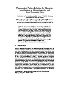
Figure 1 shows a plot of p(yi |xi ) and p(yi |x(j),i ) at one choice of xi for a typical SVR problem with d = 1. To compute the SD , further approximation of (14) is needed, resulting in SˆD (j) =

1 X DKL (p(yi |xi ); p(yi |x(j),i )). |ID |

(15)

i∈ID

Fig. 1. Demonstration of the proposed feature ranking criterion with d = 1. Dots indicate locations of yi

When p(y|x) and p(y|x(j) ) are Laplace functions or Gaussian functions, explicit expressions of SˆD (j) exist. Using (7), the KL divergence for the case of Laplace function can be shown to be L σ(j) −1 σL |f (x) − f (x(j) )| |f (x) − f (x(j) )| exp(− )+ L σL σ(j)

L DKL (pL (y|x; σ L ); pL (y|x(j) ; σ(j) )) = ln

+

σL L σ(j)

(16)

L for a given x where σ L is that given by (9) and σ(j) is obtained from (9) by replacing f (x) with f (x(j) ). Using (16) in (15) and removing associated constants yields

L SˆD (j) =

|f (xi ) − f (x(j),i )| 1 X σL [ L exp(− ) |ID | i∈I σ(j) σL

is Gaussian, the expressions are G σ(j) σG 2 2 G 2 f (x) + f (x(j) ) + (σ ) − 2f (x)f (x(j) ) 1 + − G 2 2 2(σ(j) ) 2 X (f (xi ) − f (x(j),i )) 1 G [ SˆD (j) = G 2 2|ID | i∈I (σ(j) ) G DKL (pG (y|x; σ G ); pG (y|x(j) ; σ(j) )) = ln

(18)

D

G

σ(j) σG + ( G )2 + 2 ln G ] σ σ(j)

(19)

where the expression of (18) is given by [18]. In summary, SˆD (j) can be computed for all j = 1, · · · , d, after a one-time training of SVR, one-time evaluation of σ L L G (or σ G ), d-time RP process, d-time evaluation of σ(j) (or σ(j) ) and d-time evaluation of DKL . Remark 1. The kernel matrix is different for each of the dL G time evaluation of σ(j) (or σ(j) ) and this incurs additional computations. Such computations can be kept low using update formulae. Suppose xr , xq and x(j),r , x(j),q are two samples before and after the RP process is applied to feature j. It is easy to show that K(x(j),r , x(j),q ) = K(xr , xq ) + xj(j),r ∗ xj(j),q − xjr ∗ xjq for linear kernel and K(x(j),r , x(j),q ) = K(xr , xq ) ∗ exp[κ(xjr − xjq )2 − κ(xj(j),r − xj(j),q )2 ] with kernel parameter κ for Gaussian kernel. IV. F EATURE S ELECTION S CHEME L G The proposed SˆD and SˆD can be used in two ways. The most obvious is when it is used once to yield a ranking list of all features based on a one time training of SVR on D. It can also be used for more extensive ranking schemes like the recursive feature elimination (RFE) scheme. Basically, the RFE approach works in iterations. In each iteration, a ranking of all remaining features is obtained using some appropriate L ˆG measures (SˆD , SD or others). The least important feature, as determined by the measure is then removed from further consideration. This procedure stops after n − r iterations to yield the top r features. Accordingly, the overall scheme L G with respect to measure SˆD ( SˆD ) is referred to as SD-LRFE (SD-G-RFE). Inputs to scheme SD-L-RFE are D and Γ = {1, · · · , d}, while the output is a ranked list of features in the form of an index set Γ† = {γ1† , · · · , γd† } where γj† ∈ Γ for each j = 1, · · · , d in decreasing order of importance. Following Theorem 1, the associated computational costs of the SD-L-RFE (SD-G-RFE) scheme is the training of SVR G L at each iteration and the evaluations of SˆD (j)(SˆD (j)) using (18) ((16)) for each j of the remaining features in that iteration. This is the case of the proposed scheme. In the next section where other benchmark methods are discussed, the retraining of SVR at each iteration and within the iteration may be needed for the ranking of features because of inapplicability of Theorem 1.

D

L σ(j) |f (xi ) − f (x(j),i )| + + ln L ]. L σ σ(j)

(17)

Following the same development for the case when p(y|x)

V. E XPERIMENT This section presents result of numerical experiment of SDL-RFE, SD-G-RFE and the following five existing benchmark methods on artificial and real-world data sets.

4

Mutual Information method (MI) [19]: It measures the importance of a feature by considering both the mutual information between this feature and target and the mutual information between this feature and the selected ones. Dependence maximization method (HSIC) [4]: It uses cross-covariance in the kernel space, known as the Hilbert-Schmidt norm of cross-covariance operator (HSIC) [20], as a dependence measure between feature variables and target variable. The importance of a feature is measured by its sensitivity to this dependence measure. SVM-RFE method (∆kωk2) [3], [5]: It measures the importance of a feature by the sensitivity of the cost function (1) with and without this feature. SVR radius-margin bound method (RMB) [5]: It measures the importance of a feature by its sensitivity w.r.t. SVR radius-margin bound. SVR span bound method (SpanB) [5]: It measures the importance of a feature by its sensitivity w.r.t. SVR SpanB bound.

where yi and yˆi , for i ∈ {1, · · · , |Dtst |}, are the true and predicted target values respectively . Statistical paired t-test using MSE and SCC are conducted for all problems. Specifically, paired t-test between SD-L-RFE and each of the other methods is conducted using different number of top ranked features. Herein, the null hypothesis is that the mean MSE or SCC of the two tested methods are same against the alternate hypothesis that they are not. The chance that this null hypothesis is true is measured by the returned p-value and the significance level is set at 0.05 for all experiments. The symbols “+” and “−” are used to indicate the win or loss situation of SD-L-RFE over the other tested method. In all experiments, the numerical algorithm for training of SVR is implemented by the LIBSVM package [21], where sequential minimal optimization method is used to solve the dual problem (4).

The first two benchmark methods are filter methods while the last three are wrapper methods. All methods, except mutual information method, use the same RFE scheme described in Section IV for ranking the features, and hence they are referred to as mRMR, HSIC-RFE, ∆kωk2 -RFE, RMB-RFE and SpanB-RFE, respectively. Note that the retraining of SVR within each RFE iteration is not needed for ∆kωk2 -RFE. However, in the implementation of RMB-RFE and SpanB-RFE by [5], retraining is used within each iteration of the RFE scheme. Obviously, this is much more expensive process than the proposed method since the result of Theorem 1 is not applicable to them. Our experiments include both cases: RMB-RFE and SpanB-RFE when retraining is not used and RMB-RFE* and SpanB-RFE* when it is. For each experiment data set, the result is reported over 30 realizations, which are created by random (stratified) sampling of the set D into subsets Dtrn and Dtst . As usual, Dtrn is used for SVR training, hyper-parameters tuning and feature ranking while Dtst is used for unbiased evaluation of the feature selection performance. For each realization, Dtrn is normalized to zero mean and unit standard deviation and its normalization parameters are then used to normalize Dtst . The kernel function used for all problems is Gaussian kernel. In each experiment, all hyper-parameters (C, κ, ǫ) are chosen by a 5-fold cross-validation on the first five realizations of Dtrn , and the hyper-parameters corresponding to the lowest average cross-validation error among five realizations is chosen. The grid over the (C, κ, ǫ) is [2−2 , 2−1 , · · · , 26 ] × [2−6 , 2−5 , · · · , 22 ] × [2−5 , 2−4 , · · · , 22 ]. Two well-known regression performance measures, mean squared error (MSE) and squared correlation coefficient (SCC), are used to evaluate the performance. They are given by

In this subsection, three artificial regression problems are used to evaluate the performance of every feature selection method. The first two problems were used in [22] and the last one is new. Each problem has 10 variables x1 , · · · , x10 and the target variable y depends on some of the features as given in their underlying functions: • Additive function problem

•

•

•

•

•

A. Artificial Problems

y = 0.1 exp(4x1 )+ •

4 +3x3 +2x4 +x5 +δ, 1 + exp(−20(x2 − 0.5))

Interactive function problem y = 10 sin(πx1 x2 ) + 20(x3 − 0.5) + 10x4 + 5x5 + δ,

•

Exponential function problem y = 10 exp(−((x1 )2 + (x2 )2 )) + δ,

where xj , ∀j = 1, · · · , 10 is uniformly distributed within the range [0,1] for the first two problems and [-1,1] for the last. Gaussian noise δ ∼ N (0, 0.1) for the first two problems while δ ∼ N (0, 0.2) for the last. Each artificial problem has 2000 samples. They are randomly split into Dtrn and Dtst in the ratio of |Dtrn |:|Dtst |=1:9. To investigate the effect of sparseness of the training set, decreasing sizes of |Dtrn | are also used while |Dtst | is maintained at 1800. Table I presents the number of realizations (out of 30 realizations) that relevant feature are successfully ranked as the top features by the various methods for the different settings of |Dtrn |. The best performance in each setting is highlighted in bold. From this table, the advantage of the proposed methods is clear. They generally performs as least as well if not better than all other benchmark methods except when |Dtrn | = 50 in the interactive problem,. For benchmark methods RMB-RFE* and SpanB-RFE*, the proposed methods yield comparable P|Dtst | 2 performance. It is also evident that as the size of |Dtrn | (ˆ y − y ) i i i=1 , MSE := decreases, the performance of proposed methods generally |Dtst | degrades less than that of benchmark methods. In fact, SDP P P L-RFE correctly ranks the important features in the top two (|Dtst | i yˆi yi − i yˆi i yi )2 P P P P P P SCC := (|Dtst | i yˆi2 − i yˆi i yˆi )(|Dtst | i yi2 − i yi i yi ) positions for all settings for the exponential function problem.

5

Figure 2 shows the average MSE and SCC against topranked features over 30 realizations on Dtst for exponential problem. Methods RMB-RFE and Span-RFE are not shown since they completely fail as shown in Table I. From this figure, the advantages of the proposed methods are obvious. Specifically, the proposed methods perform better than RMBRFE* and Span-RFE* when |Dtrn | = 100, 70, better than HSIC-RFE and ∆kωk2 -RFE when |Dtrn | = 50, 40, and better than mRMR for all |Dtrn |. This can be verified by aforementioned t-test. Also, it is interesting to see that the curves yielded by SD-L-RFE and SD-G-RFE constantly have one minimal MSE point (or maximal for SCC), and the unique extreme point happens when the top two features are selected. These bimodal curves strongly validate the effectiveness of the proposed feature selection methods. This is not the case for other methods. The figures for other two problems show the similar patterns and therefore not shown here. TABLE I T HE NUMBER OF REALIZATIONS THAT RELEVANT FEATURE ARE SUCCESSFULLY RANKED IN THE TOP POSITIONS OVER 30 REALIZATIONS FOR THREE ARTIFICIAL PROBLEMS . T HE BEST PERFORMANCE FOR EACH |Dtrn | IS HIGHLIGHTED IN BOLD .

Additive

Interactive

Exponential

Method\|Dtrn | SD-L-RFE SD-G-RFE mRMR HSIC-RFE ∆kωk2 -RFE RMB-RFE SpanB-RFE RMB-RFE* SpanB-RFE* Method\|Dtrn | SD-L-RFE SD-G-RFE mRMR HSIC-RFE ∆kωk2 -RFE RMB-RFE SpanB-RFE RMB-RFE* SpanB-RFE* Method\|Dtrn | SD-L-RFE SD-G-RFE mRMR HSIC-RFE ∆kωk2 -RFE RMB-RFE SpanB-RFE RMB-RFE* SpanB-RFE*

200 30 30 19 14 4 0 0 30 30 200 30 30 9 7 0 0 0 30 30 100 30 30 18 30 30 0 0 4 28

100 27 28 7 5 5 0 1 25 23 100 30 30 2 9 14 0 0 30 30 70 30 30 2 29 30 0 1 5 28

70 21 23 1 5 11 0 0 22 20 70 29 30 0 8 9 0 0 30 30 50 30 29 0 28 28 0 0 29 30

50 19 19 0 3 4 0 0 9 9 50 12 11 0 6 10 0 0 20 16 40 30 28 0 22 28 0 1 27 29

B. Real Problems Six real-world data sets from the Statlib1 , UCI repository [23] and Delve archive2 are used for evaluation purposes. Description of these data sets and the parameters used in the experiments are given in Table II. Table III shows the t-test results for all six real-world data sets. It is seen from this table that the proposed methods 1 http://lib.stat.cmu.edu/datasets/ 2 http://www.cs.toronto.edu/∼delve/data/datasets.html

TABLE II D ESCRIPTION OF REAL - WORLD DATA SETS . |Dtrn|, |Dtst |, d, C , κ AND ǫ REFER TO THE NUMBER OF TRAINING SAMPLES , NUMBER OF TEST SAMPLES , NUMBER OF FEATURES , AND SVR HYPER - PARAMETERS C , κ, ǫ RESPECTIVELY. Data sets mpg abalone cpusmall housing bodyfat triazines

|Dtrn | 353 1254 820 456 227 168

|Dtst | 39 2923 7372 50 25 18

d 7 8 12 13 14 60

C 26 26 26 26 2−2 2−1

κ 2−4 2−5 2−5 2−4 2−6 2−6

ǫ 2 2 2 2

2−5 2−3

consistently perform at least as well, if not better than all benchmark methods and the advantage is more significant for mpg, abalone, cpusmall, housing and bodyfat data sets. There two exceptions: the first few rows of data sets abalone and bodyfat show that the SD-L-RFE is statistically worse off than some benchmark methods. This should not be seen as a worrying sign as it happens for the case where one or two features are used. Clearly, this case corresponds to one of over-elimination of features. In practice, early stopping of RFE would have been triggered by the substantial increase of MSE or decrease of SCC. C. Discussion The better performance of proposed method over mRMR is expected since this common filter method is not effective in capturing effects of 3 or more interacting features. The other filter method, HSIC-RFE, appears to be quite effective in dealing with data having interacting features, and generally shows nearly comparable performance with the wrapper method ∆kωk2 -RFE. However, it is not as effective as the proposed methods from the results on artificial problems, especially when the training data is sparse, and on real-world data sets of mpg, abalone and cputime. The better performance of the proposed methods over ∆kωk2 -RFE, RMB-RFE and Span-RFE is interesting and deserves more attentions, since all of them are wrapper-based feature selection methods for SVR. The better performance of the proposed methods over them are probably attributed to the following two differences. Firstly, different ranking criteria are used. The proposed method uses the “aggregate” sensitivity of SVR probabilistic predictions with respect to a feature over the feature space while ∆kωk2 RFE uses the sensitivity of the cost function of SVR with respect to a feature and RMB-RFE and Span-RFE uses the sensitivity of the error bound of SVR with respect to a feature. Secondly, ∆kωk2 -RFE, RMB-RFE and Span-RFE assumes that the SVR solution remains unchanged when a feature is removed within each RFE iteration. This appears to be a strong assumption, judging from the relative performances of RMBRFE, Span-RFE RMB-RFE* and Span-RFE*. Another advantage of the proposed method is the modest computational load. As mentioned in Section 3, the evaluation of scores for d features includes a one-time training of SVR of about O(n2.3 ) [24] complexity, one-time evaluation of σ L (or σ G ) of O(mn) where n = |D|, m is the number of support L vectors, d-time RP process of O(dn), d-time evaluation of σ(j)

6

0 1

2

3 4 5 6 7 8 Number of Top−ranked Features

9

10

0.4 0.2 1

2

exponential−50

10

1

3 4 5 6 7 8 Number of Top−ranked Features

9

10

0.8 0.6 0.4

2

3 4 5 6 7 8 Number of Top−ranked Features

1 2

3 4 5 6 7 8 Number of Top−ranked Features

9

10

0.8 0.6 0.4 0.2 1

2

9

10

5 4 3 2 1 0 1

2

3 4 5 6 7 8 Number of Top−ranked Features

3 4 5 6 7 8 Number of Top−ranked Features

9

10

9

10

exponential−40

6

1

0.2 1

2

1

exponential−40

Mean squared error

2

Squared correlation coefficient

Mean squared error

3

2

9

3

0 1

exponential−50

4

0 1

SD−L−RFE SD−G−RFE mRMR HSIC−RFE ∆ ||w||2−RFE RMB−RFE* SpanB−RFE* 3 4 5 6 7 8 Number of Top−ranked Features

4

Squared correlation coefficient

1

0.8 0.6

exponential−70

5

1 Mean squared error

2

Squared correlation coefficient

Mean squared error

3

exponential−70

exponential−100

SD−L−RFE SD−G−RFE mRMR HSIC−RFE ∆ ||w||2−RFE RMB−RFE* SpanB−RFE*

9

10

Squared correlation coefficient

exponential−100 4

1 0.8 0.6 0.4 0.2 0 1

2

3 4 5 6 7 8 Number of Top−ranked Features

Fig. 2. Average MSE (left-hand side) and average SCC (right-hand side) against top-ranked features over 30 realizations for Exponential Function Problem with six different settings

G (or σ(j) ) of O(dmn), and d-time evaluation of DKL of O(dn). Hence, after one-time training SVR, the proposed criterion scales linearly with respect to d and n. Obviously, ∆kωk2 RFE, RMB-RFE and Span-RFE have similar computational cost like the proposed methods. However, RMB-RFE* and Span-RFE* require the training of SVR d − 1 times more than the proposed methods when evaluating the scores for d features. This additional computational load is of O(dn2.3 ), which is significant when n is large.

VI. C ONCLUSIONS This paper presents a new wrapper-based feature selection method for SVR. This method measures the importance of a feature by the aggregation, over the feature space, of the sensitivity of SVR probabilistic prediction with and without the feature. Two approximations of the criterion with random permutation process are proposed. The numerical experiment on both artificial and real-world problems suggests that the proposed method generally performs as least as well, if not better than three benchmark methods. The advantage of the proposed methods is more significant when the training data is sparse, or has a low samples-to-features ratio. As a wrapper method, the computational cost of proposed methods is moderate. R EFERENCES [1] A. Blum and P. Langley, “Selection of relevant features and examples in machine learning,” Artificial Intelligence, vol. 97, no. 1-2, pp. 245–271, 1997. [2] R. Kohavi and G. H. John, “Wrappers for feature selection,” Artificial Intelligence, vol. 97, no. 1-2, pp. 273–324, 1997. [3] I. Guyon, J. Weston, S. Barnhill, and V. Vapnik, “Gene selection for cancer classification using support vector machines,” Machine Learning, vol. 46, no. 1-3, pp. 389–422, 2002. [4] L. Song, A. Smola, A. Gretton, J. Bedo, and K. Borgwardt, “Supervised feature selection via dependence estimation,” in ICML ’07: Proceedings of the 24th international conference on Machine learning. New York, NY, USA: ACM, 2007, pp. 823–830. [5] A. Rakotomamonjy, “Analysis of svm regression bounds for variable ranking,” Neurocomputing, vol. 70, no. 7-9, pp. 1489 – 1501, 2007. [6] R. Tibshirani, “Regression shrinkage and selection via the lasso,” Journal of the Royal Statistical Society. Series B, vol. 58, no. 1, pp. 267–288, 1996. [7] A. Rakotomamonjy, “Variable selection using SVM-based criteria,” Journal of Machine Learning Research, vol. 3, pp. 1357–1320, 2003.

[8] K.-Q. Shen, C.-J. Ong, X.-P. Li, and E. P. Wilder-Smith, “Feature selection via sensitivity analysis of SVM probabilistic outputs,” Machine Learning, vol. 70, no. 1, pp. 1–20, 2008. [9] J.-B. Yang, K.-Q. Shen, C.-J. Ong, and X.-P. Li, “Feature selection for mlp neural network: The use of random permutation of probabilistic outputs,” IEEE Transactions on Neural Networks, vol. 20, no. 12, pp. 1911–1922, 2009. [10] A. J. Smola and B. Scholkopf, “A tutorial on support vector regression,” Statistics and Computing, vol. 14, no. 3, pp. 199–222, 2004. [11] D. MacKay, “The evidence framework applied to classification networks,” Neural Computation, vol. 4, no. 5, pp. 720–736, 1992. [12] M. H. Law and J. T. Kwok, “Bayesian support vector regression,” in In Proceedings of the Eighth International Workshop on Artificial Intelligence and Statistics, 2001, pp. 239–244. [13] J. B. Gao, S. R. Gunn, C. J. Harris, and M. Brown, “A probabilistic framework for SVM regression and error bar estimation,” Machine Learning, vol. 46, no. 1-3, pp. 71–89, 2002. [14] W. Chu, S. S. Keerthi, and C. J. Ong, “Bayesian support vector regression using a unified loss function,” IEEE Transactions on Neural Networks, vol. 15, pp. 29–44, 2004. [15] C. J. Lin and R. C. Weng, “Simple probabilistic predictions for support vector regression,” Department of Cmputer Science, National Taiwan University, Tech. Rep., 2004. [16] C. M. Bishop, Neural Networks for Pattern Recognition. Oxford University Press, November 1995. [17] Page.E.S., “A note on generating random permutations,” Applied Statistics, vol. 16, no. 3, pp. 273–274, 1967. [18] W. Penny, “Kullback-Liebler divergences of Normal, Gamma, Dirichlet and Wishart densities,” Wellcome Department of Cognitive Neurology, University College London, Tech. Rep., 2001. [19] F.H.Long, H.C.Peng, and C.Ding, “Feature selection based on mutual information: criteria of max-dependency ,max-relevance, and minredundancy,” IEEE Transactions on Pattern Analysis and Machine Intelligence, vol. 27, no. 8, pp. 1226–1238, August 2005. [20] A. Gretton, O. Bousquet, A. Smola, and B. Schoelkopf, “Measuring statistical dependence with Hilbert-Schmidt norms,” in ALT 2005, 10/08/ 2005, pp. 63–78. [21] C.-C. Chang and C.-J. Lin, LIBSVM: a library for support vector machines, 2001. [Online]. Available: http://www.csie.ntu.edu.tw/∼cjlin/libsvm [22] J. H. Friedman, “Multivariate adaptive regression splines,” The Annals of Statistics, vol. 19, no. 1, pp. 1–67, 1991. [23] A.Asuncion and D.J.Newman, “UCI machine learning repository,” 2007. [Online]. Available: http://www.ics.uci.edu/∼mlearn/MLRepository.html [24] J. C. Platt, Using sparseness and analytic QP to speed training of support vector machines. Cambridge, MIT Press, 1998, ch. In M.S. Kearns, S.A. Solla and D. A. Cohn (Eds), Advances in Neural Information Processing Systems, 11.

7

TABLE III t- TEST ON REAL - WORLD DATA SET. T HE p- VALUES LESS THAN 0.05 ARE HIGHLIGHTED IN BOLD . N

Dataset

mpg

abalone

cpusmall

housing

bodyfat

triazines

mpg

abalone

cpusmall

housing

bodyfat

triazines

N

SD-L-RFE mean value

SD-G-RFE mean pvalue value

mRMR mean pvalue value

1 2 3 4 5 6 7 1 2 3 4 5 6 7 8 2 4 6 8 10 12 2 4 6 8 10 12 13 2 4 6 8 10 12 14 1 10 20 30 40 50 60

16.47 7.71 6.76 6.81 6.82 6.68 6.20 6.73 4.95 4.74 4.69 4.67 4.64 4.62 4.57 40.39 18.99 19.20 20.66 21.64 23.78 19.00 16.00 13.74 11.47 9.57 10.12 10.48 .00022 .00018 .00021 .00020 .00020 .00021 .00021 0.020 0.018 0.017 0.017 0.018 0.018 0.018

16.47 7.71 6.76 6.81 6.82 6.70 6.20 6.67 4.95 4.74 4.69 4.67 4.64 4.62 4.57 64.81 19.33 19.22 21.28 22.52 23.78 19.00 15.94 13.59 12.46 10.76 10.12 10.48 .00022 .00018 .00021 .00020 .00020 .00021 .00021 0.020 0.017 0.017 0.018 0.018 0.018 0.018

1.00 1.00 1.00 1.00 1.00 0.98 1.00 0.63 0.95 1.00 0.99 0.95 0.87 0.98 1.00 0.00+ 0.55 0.97 0.32 0.24 1.00 1.00 0.98 0.94 0.54 0.40 1.00 1.00 0.91 0.93 1.00 0.97 0.99 1.00 1.00 1.00 0.92 0.98 0.83 0.94 0.99 1.00

16.86 16.32 15.51 13.46 11.84 6.68 6.20 6.10 6.02 5.39 5.39 5.34 5.21 4.59 4.58 297.51 279.65 116.14 19.69 20.68 23.78 29.36 25.46 16.28 15.24 11.32 9.45 10.48 .00017 .00016 .00019 .00023 .00023 .00023 .00021 0.020 0.017 0.018 0.018 0.018 0.018 0.018

0.75 0.00+ 0.00+ 0.00+ 0.00+ 1.00 1.00 0.000.00+ 0.00+ 0.00+ 0.00+ 0.00+ 0.32 1.00 0.00+ 0.00+ 0.00+ 0.07 0.15 1.00 0.00+ 0.00+ 0.26 0.06 0.18 0.62 1.00 0.000.07 0.08 0.04 0.05 0.16 1.00 0.95 0.84 0.75 0.63 0.98 0.91 1.00

1 2 3 4 5 6 7 1 2 3 4 5 6 7 8 2 4 6 8 10 12 2 4 6 8 10 12 13 2 4 6 8 10 12 14 1 10 20 30 40 50 60

0.73 0.87 0.89 0.89 0.89 0.89 0.90 0.36 0.53 0.55 0.55 0.55 0.56 0.56 0.56 0.89 0.95 0.95 0.94 0.94 0.93 0.77 0.80 0.83 0.86 0.88 0.88 0.87 0.89 0.84 0.79 0.80 0.75 0.74 0.73 0.12 0.26 0.28 0.29 0.26 0.25 0.25

0.73 0.87 0.89 0.89 0.89 0.89 0.89 0.36 0.53 0.55 0.55 0.56 0.56 0.56 0.56 0.82 0.95 0.95 0.94 0.94 0.93 0.77 0.80 0.83 0.85 0.87 0.88 0.87 0.89 0.84 0.79 0.80 0.75 0.74 0.73 0.12 0.27 0.29 0.26 0.26 0.25 0.25

1.00 1.00 1.00 1.00 1.00 0.98 1.00 0.63 0.95 1.00 0.99 0.95 0.87 0.98 1.00 0.00+ 0.55 0.97 0.32 0.24 1.00 1.00 0.98 0.94 0.54 0.40 1.00 1.00 0.91 0.93 1.00 0.97 0.99 1.00 1.00 1.00 0.92 0.98 0.83 0.94 0.99 1.00

0.72 0.73 0.74 0.78 0.81 0.89 0.90 0.42 0.42 0.49 0.49 0.49 0.50 0.56 0.56 0.16 0.21 0.67 0.94 0.94 0.93 0.65 0.70 0.80 0.82 0.86 0.88 0.87 0.95 0.92 0.84 0.79 0.76 0.73 0.73 0.08 0.25 0.22 0.20 0.26 0.26 0.25

0.75 0.00+ 0.00+ 0.00+ 0.00+ 1.00 1.00 0.000.00+ 0.00+ 0.00+ 0.00+ 0.00+ 0.32 1.00 0.00+ 0.00+ 0.00+ 0.07 0.15 1.00 0.00+ 0.00+ 0.26 0.06 0.18 0.62 1.00 0.000.07 0.08 0.05 0.05 0.16 1.00 0.95 0.84 0.75 0.62 0.98 0.90 1.00

HSIC-RFE ∆kωk2 -RFE mean pmean pvalue value value value MSE measure 22.45 0.00+ 16.47 1.00 18.06 0.00+ 7.71 1.00 15.67 0.00+ 7.54 0.22 13.46 0.00+ 6.88 0.91 9.79 0.00+ 6.71 0.86 6.44 0.67 6.63 0.92 6.20 1.00 6.20 1.00 6.15 0.006.27 0.005.90 0.00+ 4.97 0.51 5.62 0.00+ 4.80 0.05 5.41 0.00+ 4.72 0.42 5.29 0.00+ 4.66 0.88 5.28 0.00+ 4.63 0.67 4.90 0.00+ 4.60 0.62 4.57 1.00 4.57 1.00 293.6 0.00+ 75.45 0.00+ 82.44 0.00+ 60.09 0.00+ 28.57 0.32 39.89 0.00+ 20.49 0.78 29.36 0.00+ 22.49 0.28 25.61 0.00+ 23.78 1.00 23.78 1.00 19.00 1.00 28.99 0.00+ 14.86 0.60 15.19 0.71 13.90 0.94 13.69 0.98 11.54 0.96 12.02 0.74 10.49 0.50 11.08 0.28 9.51 0.65 10.36 0.87 10.48 1.00 10.48 1.00 .00022 0.91 .00022 0.91 .00025 0.00+ .00017 0.19 .00026 0.00+ .00020 0.29 .00026 0.05 .00020 0.95 .00025 0.05 .00020 0.95 .00025 0.05 .00020 0.66 .00021 1.00 .00021 1.00 0.021 0.95 0.021 0.69 0.019 0.63 0.018 0.80 0.017 0.89 0.017 0.87 0.017 0.94 0.017 0.95 0.018 0.75 0.017 0.85 0.020 0.52 0.018 0.93 0.018 1.00 0.018 1.00 SCC measure 0.63 0.00+ 0.73 1.00 0.70 0.00+ 0.87 1.00 0.74 0.00+ 0.88 0.22 0.78 0.00+ 0.89 0.91 0.84 0.00+ 0.89 0.86 0.90 0.67 0.89 0.92 0.89 1.00 0.89 1.00 0.41 0.000.40 0.000.44 0.00+ 0.53 0.51 0.46 0.00+ 0.54 0.05 0.48 0.00+ 0.55 0.42 0.50 0.00+ 0.56 0.88 0.50 0.00+ 0.56 0.67 0.53 0.00+ 0.56 0.62 0.56 1.00 0.56 1.00 0.17 0.00+ 0.79 0.00+ 0.77 0.00+ 0.83 0.00+ 0.92 0.32 0.89 0.00+ 0.94 0.78 0.92 0.00+ 0.94 0.28 0.93 0.00+ 0.93 1.00 0.93 1.00 0.77 1.00 0.65 0.00+ 0.82 0.60 0.81 0.71 0.83 0.94 0.83 0.98 0.86 0.96 0.85 0.74 0.87 0.50 0.86 0.28 0.88 0.65 0.87 0.87 0.87 1.00 0.87 1.00 0.89 0.91 0.89 0.91 0.83 0.00+ 0.86 0.19 0.80 0.00+ 0.81 0.29 0.79 0.05 0.78 0.95 0.77 0.05 0.76 0.95 0.76 0.05 0.75 0.66 0.73 1.00 0.73 1.00 0.08 0.95 0.07 0.69 0.19 0.63 0.22 0.80 0.26 0.89 0.28 0.87 0.26 0.94 0.29 0.95 0.22 0.75 0.27 0.85 0.17 0.52 0.26 0.93 0.25 1.00 0.25 1.00

IS THE NUMBER OF TOP RANKED FEATURES .

RMB-RFE mean pvalue value

SpanB-RFE mean pvalue value

RMB-RFE* mean pvalue value

SpanB-RFE* mean pvalue value

22.45 17.77 17.39 15.71 13.62 11.16 6.20 7.15 6.37 5.16 4,83 4.73 4.71 4.63 4.58 276.56 242.23 167.24 19.96 20.81 23.78 64.09 38.98 28.96 24.63 12.25 10.81 10.48 .00021 .00021 .00021 .00022 .00022 .00023 .00021 0.021 0.020 0.020 0.019 0.018 0.018 0.018

0.00+ 0.00+ 0.00+ 0.00+ 0.00+ 0.00+ 1.00 0.00+ 0.00+ 0.00+ 0.00+ 0.17 0.16 0.78 1.00 0.00+ 0.00+ 0.00+ 0.25 0.25 1.00 0.00+ 0.00+ 0.00+ 0.00+ 0.07 0.63 1.00 0.51 0.11 0.88 0.31 0.14 0.27 1.00 0.65 0.25 0.15 0.30 0.83 0.93 1.00

31.79 18.35 16.29 14.30 13.51 8.62 6.20 6.97 6.82 6.29 5.87 5.29 4.89 4.71 4.58 141.00 32.66 16.60 17.54 19.67 23.78 62.60 56.52 50.93 43.99 37.94 17.83 10.48 .00026 .00023 .00021 .00023 .00023 .00022 .00021 0.021 0.021 0.021 0.020 0.019 0.019 0.018

0.00+ 0.00+ 0.00+ 0.00+ 0.00+ 0.04+ 1.00 0.01+ 0.00+ 0.00+ 0.00+ 0.00+ 0.00+ 0.07 1.00 0.00+ 0.15 0.05 0.06 0.07 1.00 0.00+ 0.00+ 0.00+ 0.00+ 0.00+ 0.00+ 1.00 0.08 0.02+ 0.16 0.09 0.12 0.48 1.00 0.65 0.18 0.11 0.17 0.43 0.73 1.00

22.21 17.75 17.31 15.96 13.96 11.17 6.20 7.12 6.67 5.96 5.73 5.28 4.88 4.63 4.58 295.11 222.18 112.87 78.51 55.55 23.78 46.80 23.22 18.33 11.38 11.71 10.81 10.48 .00032 .00020 .00019 .00019 .00019 .00020 .00021 0.021 0.020 0.020 0.020 0.019 0.019 0.018

0.00+ 0.00+ 0.00+ 0.00+ 0.00+ 0.00+ 1.00 0.00+ 0.00+ 0.00+ 0.00+ 0.00+ 0.00+ 0.79 1.00 0.00+ 0.00+ 0.00+ 0.00+ 0.00+ 1.00 0.00+ 0.01+ 0.03+ 0.95 0.15 0.65 1.00 0.00+ 0.28 0.12 0.54 0.78 0.59 1.00 0.65 0.20 0.14 0.23 0.46 0.72 1.00

16.97 8.59 7.69 7.30 6.65 6.50 6.20 6.18 4.95 4.87 4.79 4.76 4.70 4.67 4.58 291.26 247.39 206.61 124.44 59.30 23.78 19.00 13.97 12.63 11.34 11.60 10.69 10.48 .00018 .00022 .00024 .00025 .00024 .00023 .00021 0.021 0.018 0.017 0.018 0.018 0.018 0.018

0.69 0.25 0.15 0.41 0.78 0.63 1.00 0.000.92 0.00+ 0.00+ 0.01+ 0.06 0.12 1.00 0.00+ 0.00+ 0.00+ 0.00+ 0.00+ 1.00 1.00 0.35 0.54 0.93 0.18 0.70 1.00 0.000.04+ 0.06 0.00+ 0.01+ 0.19 1.00 0.85 0.89 0.93 0.97 0.94 0.96 1.00

0.63 0.70 0.71 0.74 0.78 0.82 0.90 0.32 0.39 0.51 0.54 0.55 0.55 0.56 0.56 0.22 0.31 0.52 0.94 0.94 0.93 0.23 0.54 0.66 0.71 0.85 0.86 0.87 0.52 0.73 0.79 0.79 0.78 0.76 0.73 0.094 0.11 0.12 0.18 0.25 0.22 0.25

0.00+ 0.00+ 0.00+ 0.00+ 0.00+ 0.00+ 1.00 0.00+ 0.00+ 0.00+ 0.02+ 0.17 0.16 0.78 1.00 0.00+ 0.00+ 0.00+ 0.25 0.25 1.00 0.00+ 0.00+ 0.00+ 0.00+ 0.07 0.63 1.00 0.51 0.11 0.88 0.31 0.14 0.27 1.00 0.65 0.25 0.15 0.30 0.83 0.94 1.00

0.48 0.69 0.73 0.76 0.78 0.86 0.90 0.33 0.35 0.40 0.44 0.50 0.53 0.55 0.56 0.60 0.91 0.95 0.95 0.94 0.93 0.25 0.34 0.41 0.49 0.56 0.79 0.87 0.38 0.46 0.47 0.48 0.53 0.57 0.73 0.11 0.11 0.12 0.14 0.17 0.19 0.25

0.00+ 0.00+ 0.00+ 0.00+ 0.00+ 0.04+ 1.00 0.01+ 0.00+ 0.00+ 0.00+ 0.00+ 0.00+ 0.07 1.00 0.00+ 0.15 0.05 0.06 0.07 1.00 0.00+ 0.00+ 0.00+ 0.00+ 0.00+ 0.00+ 1.00 0.08 0.02+ 0.16 0.09 0.12 0.48 1.00 0.85 0.18 0.11 0.17 0.43 0.73 1.00

0.63 0.71 0.71 0.74 0.86 0.82 0.90 0.32 0.36 0.43 0.45 0.50 0.54 0.56 0.56 0.17 0.37 0.68 0.78 0.84 0.93 0.45 0.73 0.79 0.86 0.86 0.87 0.87 0.18 0.58 0.80 0.78 0.76 0.75 0.73 0.094 0.12 0.14 0.17 0.17 0.21 0.25

0.00+ 0.00+ 0.00+ 0.00+ 0.00+ 0.00+ 1.00 0.00+ 0.00+ 0.00+ 0.00+ 0.00+ 0.00+ 0.78 1.00 0.00+ 0.00+ 0.00+ 0.00+ 0.00+ 1.00 0.00+ 0.01+ 0.03+ 0.95 0.15 0.64 1.00 0.00+ 0.28 0.12 0.54 0.78 0.59 1.00 0.65 0.20 0.14 0.23 0.46 0.72 1.00

0.72 0.86 0.87 0.88 0.89 0.90 0.90 0.41 0.53 0.54 0.54 0.55 0.55 0.53 0.56 0.17 0.29 0.41 0.65 0.84 0.93 0.77 0.83 0.84 0.86 0.86 0.86 0.87 0.79 0.75 0.75 0.73 0.73 0.75 0.73 0.11 0.26 0.30 0.28 0.27 0.26 0.25

0.69 0.25 0.15 0.41 0.78 0.63 1.00 0.000.92 0.00+ 0.00+ 0.01+ 0.06 0.12 1.00 0.00+ 0.00+ 0.00+ 0.00+ 0.00+ 1.00 1.00 0.35 0.54 0.93 0.18 0.70 1.00 0.00+ 0.04+ 0.06 0.00+ 0.01+ 0.19 1.00 0.85 0.89 0.93 0.97 0.94 0.96 1.00