Feature Selection for Ranking 1,2

1

1,3

1

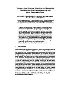
Xiubo Geng *, Tie-Yan Liu , Tao Qin *, Hang Li 1

Microsoft Research Asia, No.49 Zhichun Road, Haidian District, Beijing 100080, P.R. China Institue of Computing Technology, Chinese Academy of Sciences, Beijing, 100080, P.R. China 3 Dept. Electronic Engineering, Tsinghua University, Beijing, 100084, P.R. China 1 {tyliu, hangli}@microsoft.com 2 [email protected] 3 [email protected]

2

ABSTRACT Ranking is a very important topic in information retrieval. While algorithms for learning ranking models have been intensively studied, this is not the case for feature selection, despite of its importance. The reality is that many feature selection methods used in classification are directly applied to ranking. We argue that because of the striking differences between ranking and classification, it is better to develop different feature selection methods for ranking. To this end, we propose a new feature selection method in this paper. Specifically, for each feature we use its value to rank the training instances, and define the ranking accuracy in terms of a performance measure or a loss function as the importance of the feature. We also define the correlation between the ranking results of two features as the similarity between them. Based on the definitions, we formulate the feature selection issue as an optimization problem, for which it is to find the features with maximum total importance scores and minimum total similarity scores. We also demonstrate how to solve the optimization problem in an efficient way. We have tested the effectiveness of our feature selection method on two information retrieval datasets and with two ranking models. Experimental results show that our method can outperform traditional feature selection methods for the ranking task.

Categories and Subject Descriptors H.3.3 [Information Search and Retrieval]: Information Search and Retrieval – Selection process.

General Terms Algorithms, Performance, Experimentation, Theory

Keywords Information retrieval, learning to rank, feature selection

1. INTRODUCTION Ranking is a central issue in information retrieval, in which given *The work was done when the first and the third authors were interns at Microsoft Research Asia. Permission to make digital or hard copies of all or part of this work for personal or classroom use is granted without fee provided that copies are not made or distributed for profit or commercial advantage and that copies bear this notice and the full citation on the first page. To copy otherwise, or republish, to post on servers or to redistribute to lists, requires prior specific permission and/or a fee. SIGIR’07, July 23–27, 2007, Amsterdam, Holland. Copyright 2007 ACM 1-58113-000-0/00/0004…$5.00.

a set of objects (e.g., documents), a score for each of them is computed and the objects are sorted according to the scores. Depending on applications the scores may represent the degrees of relevance, preference, or importance. In this paper, without loss of generality, we take ranking in relevance search as example. Traditionally only a small number of strong features (e.g., BM25 [25] and language model [17][23]) were used to represent relevance and to rank documents. In recent years, with the development of the supervised learning algorithms like Ranking SVM [10][13] and RankNet [4], it becomes possible to incorporate more features (strong or weak) into ranking models. In this situation, feature selection inevitably becomes an important issue, particularly from the following viewpoints. First, feature selection can help enhance accuracy in many machine learning problems, which strongly indicates that feature selection is also necessary for ranking. For example, although the generalization ability of Support Vector Machines (SVM) depends on margin which does not change with the addition of irrelevant features, it also depends on the radius of training data points, which can increase when the number of features [19][5][29] increases. Moreover, the probability of over-fitting also increases as the dimension of feature space increases, and feature selection is a powerful means to avoid over-fitting [22]. Second, feature selection can also help improve the efficiency of training. In information retrieval, especially in web search, usually the data size is very large and thus training of ranking models is computationally costly. For example, when applying Ranking SVM to web search, it is easy to encounter a situation in which training cannot be completed in an acceptable time period (c.f., [12]). To cope with the problem, we can conduct feature selection before training, because the complexities of most learning algorithms are proportional to the number of features. Although feature selection is important, to our knowledge, there have been no methods of feature selection dedicatedly proposed for ranking. Most of the methods used in ranking were developed for classification. Basically, feature selection methods in classification fall into three categories [8]. In the first category, which is named filter, feature selection is defined as a preprocessing step and can be independent from learning. A filter method computes a score for each feature and then selects features according to the scores [20]. Yang et al [31] and Forman [7] conducted comparative studies on filter methods, and they found that information gain (IG) and chi-square (CHI) are among the most effective methods of feature selection for classification. The second category referred to as wrapper [15] utilizes the learning system as a black box to score subsets of features, and the third

category called the embedded method [3] performs feature selection within the process of training. Among these three categories, the most comprehensively-studied methods are the filter methods. Therefore, we also base our discussions on this category in this paper, and we will use “feature selection” and “the filter methods for feature selection” interchangeably. When applying the feature selection methods to ranking, several problems may arise. First, there is a significant gap between classification and ranking. In ranking, a number of ordered categories are used, representing the ranking relationship between instances, while in classification the categories are “flat”. Obviously, existing feature selection methods for classification are not suitable for ranking. Second, the evaluation measures (e.g. mean average precision (MAP) [32] and normalized discounted cumulative gain (NDCG) [11]) used in ranking problems are different from those measures used in classification: 1) in ranking usually precision is more important than recall [32] while in classification both precision and recall are important; 2) in ranking correctly ranking the top-n instances is more critical [11] while in classification making a correct classification decision is of equal significance for all instances. These differences indicate the necessity of developing new techniques for feature selection in ranking. In this paper, we propose a novel method for this purpose with the following properties. 1)

The method makes use of ranking information, instead of simply viewing the ranks as flat categories. For example, it uses evaluation measures or loss functions [4][10] in ranking to measure the importance of features.

2)

Inspired by the work in [1][14][27], it considers the similarities between features, and tries to avoid selecting redundant features.

3)

It models feature selection for ranking as a multi-objective optimization problem. The final objective is to find a set of features with maximum importance and minimum similarity.

4)

It provides a greedy search algorithm to solve the optimization problem. The corresponding solution produced is proven to be equivalent to the optimal solution to the original problem under certain condition.

We believe that these properties are essential for feature selection in ranking. We have tested the performance of the proposed feature selection method on two datasets (OHSUMED [9] and .gov in TREC2004 [28]) and with two state-of-the-art ranking models (Ranking SVM [10] and RankNet [4]). Experimental results show that the proposed method can outperform traditional feature selection methods in the task of ranking for information retrieval. The rest of the paper is organized as follows. Section 2 introduces our feature selection method. Section 3 describes the experimental settings, and the experimental results are reported in Section 4. Section 5 summarizes the major findings in this work, and lists potential future work.

2. FEATURE SELECTION METHOD 2.1 Overview

Suppose the goal is to select 𝑡(1 ≤ 𝑡 ≤ 𝑚) features from the entire feature set {𝑣1 , 𝑣2 , … , 𝑣𝑚 }. In our method we first define the importance score of each feature 𝑣𝑖 , and define the similarity between any two features 𝑣𝑖 and 𝑣𝑗 . Then we employ an efficient algorithm to maximize the total importance scores and minimize the total similarity scores of a set of features.

2.2 Importance of feature We first assign an importance score to each feature. Specifically, we propose using an evaluation measure like MAP and NDCG (the definitions of them will be given in Section 3) or a loss function (e.g. pair-wise ranking errors [10][13]) to compute the importance score. In the former, we first rank instances using the feature, evaluate the performance in terms of the measure, and then take the evaluation result as the importance score. In the latter, we also rank instances using the feature, and then view a score inversely proportional to the corresponding loss as the importance score. Note that for some features larger values correspond to higher ranks while for other features smaller values correspond to higher ranks, when calculating MAP, NDCG or the loss of ranking models, we actually sort the instances for two times (in the normal order and in the inverse order), and take the larger score as the importance score of the feature.

2.3 Similarity between features Inspired by the work in [1][14][27], we also consider removing redundancy in the selected features. This is particularly necessary in the cases in which we are required to only utilize a small number of features. In this work, we measure the similarity between any two features on the basis of their ranking results. That is, we regard each feature as a ranking model, and the similarity between two features is represented by the similarity between the ranking results that they produce. Many methods have been proposed to measure the distance between two ranking results (ranking lists), such as Spearman’s footrule F, rank correlation R, and Kendall’s 𝜏 [16][18]. In principle all of them can be used here, and in this paper we choose Kendall’s 𝜏 as an example. The Kendall’s 𝜏 value of query q for any two features 𝑣𝑖 and 𝑣𝑗 can be calculated as follows, 𝜏𝑞 𝑣𝑖 , 𝑣𝑗 =

# 𝑑 𝑠 ,𝑑 𝑡 ∈𝐷𝑞 𝑑 𝑠 ≺𝑣𝑖 𝑑 𝑡 𝑎𝑛𝑑 𝑑 𝑠 ≺𝑣𝑗 𝑑 𝑡 } #{ 𝑑 𝑠 ,𝑑 𝑡 ∈𝐷𝑞 }

where 𝐷𝑞 denotes the set of instance pairs 𝑑𝑠 , 𝑑𝑡 in response with respect to query q, #{∙} represents the number of elements in a set, and 𝑑𝑠 ≺𝑣𝑖 𝑑𝑡 implies that instance 𝑑𝑡 is ranked ahead of instance 𝑑𝑠 by feature vi. For a set of queries, the Kendall’s 𝜏 va lues of all the queries are averaged, and the result 𝜏 𝑣𝑖 , 𝑣𝑗 is used as the final similarity score between features 𝑣𝑖 and 𝑣𝑗 . It is easy to see that 𝜏 𝑣𝑖 , 𝑣𝑗 = 𝜏 𝑣𝑗 , 𝑣𝑖 holds.

2.4 Optimization formulation As aforementioned, we want to select those features with largest total importance scores and smallest total similarity scores. Mathematically, this can be represented as follows:

max min 𝑠. 𝑡.

𝑖

𝑖 𝜔𝑖

𝑥𝑖

𝑗 ≠𝑖 𝑒𝑖,𝑗 𝑥𝑖 𝑥𝑗

𝑥𝑖 𝜖 0,1 𝑖 = 1, … , 𝑚 𝑖 𝑥𝑖

(1)

=𝑡

Here 𝑡 denotes the number of selected features, 𝑥𝑖 = 1 (or 0) indicates that feature 𝑣𝑖 is selected (or not), 𝜔𝑖 denotes the importance score of feature 𝑣𝑖 , and 𝑒𝑖,𝑗 denotes the similarity between feature 𝑣𝑖 and feature 𝑣𝑗 . In this paper, we let 𝑒𝑖,𝑗 = 𝜏 𝑣𝑖 , 𝑣𝑗 , and obviously 𝑒𝑖,𝑗 = 𝑒𝑗 ,𝑖 . In (1), there are two objectives: to maximize the sum of the importance scores of individual features, and to minimize the sum of similarity scores between any two features. Since multiobjective programming is not easy to solve, we take a common approach in optimization and convert multi-objective programming to single-objective programming using linear combination. max

𝑖 𝜔𝑖

𝑥𝑖 − 𝑐

𝑖

(2)

Here c is a parameter to balance the two objectives.

2.5 Solution to optimization problem The optimization in (2) is a typical 0-1 integer programming problem. As far as we know, there is no efficient solution to such kind of problem. One possible approach would be to perform exhaustive search. However, the time complexity of it, 𝑂(𝐶𝑚𝑡 ), is too high to make it applicable in real applications. We need to look for more practical solutions. In this work, we propose a greedy search algorithm for tackling the issue, as in Fig.1. Algorithm GAS (Greedy search Algorithm of feature Selection)

3.

Construct an undirected graph G0, in which each node represents a feature, the weight of node 𝑣𝑖 is 𝜔𝑖 and the weight of an edge between node 𝑣𝑖 and node 𝑣𝑗 is 𝑒𝑖,𝑗 . Construct a set S to contain the selected features. Initially S0 = ∅. For i = 1…t, (1) Select the node with the largest weight, without loss of generality, suppose that the selected node is 𝑣𝑘 𝑖 . (2) A punishment is conducted on all the other nodes according to their similarities with 𝑣𝑘 𝑖 . That is, the weights of all the other nodes are updated as follows. 𝜔𝑗 ← 𝜔𝑗 − 𝑒𝑘 𝑖 ,𝑗 ∗ 2𝑐, 𝑗 ≠ 𝑘𝑖 (3) Add 𝑣𝑘 𝑖 to the set S and remove it from graph G together with all the edges connected to it: 𝑆𝑖+1 = 𝑆𝑖 ⋃{𝑣𝑘 𝑖 }, 𝐺𝑖+1 = 𝐺𝑖 \{𝑣𝑘 𝑖 }

4.

Proof: The condition 𝑆𝑡+1 ⊃ 𝑆𝑡 indicates that when selecting the (t+1)-th feature, we do not change the already-selected t features. Denote 𝑆𝑡 = {𝑣𝑘 𝑖 |𝑖 = 1, … , 𝑡} , where 𝑣𝑘 𝑖 is the ki-th feature selected in the i-th iteration. Then the task turns out to be that of finding the (t+1)-th feature so that the following objective can be met. max

Output St. Fig.1 Greedy algorithm of feature selection for ranking

The time complexity of the proposed algorithm is of order O(mt), and thus the algorithm is efficient. Furthermore, as made clear in

t+1 i=1 𝜔𝑘 𝑖

–𝑐

𝑡+1 𝑖=1

𝑗 ≠𝑖 𝑒𝑘 𝑖 ,𝑘 𝑗

(3)

Since 𝑒𝑘 𝑖 ,𝑘 𝑗 = 𝑒𝑘 𝑗 ,𝑘 𝑖 , we can rewrite (3) as max

𝑖 𝑥𝑖 = 𝑡

2.

Theorem 1: With the greedy search algorithm in Fig.1 one can find the optimal solution to problem (2), provided that 𝑆𝑡+1 ⊃ 𝑆𝑡 , where 𝑆𝑡 denotes the selected feature set with 𝑆 = 𝑡.

𝑗 ≠𝑖 𝑒𝑖,𝑗 𝑥𝑖 𝑥𝑗

𝑠. 𝑡. 𝑥𝑖 𝜖 0,1 𝑖 = 1, … , 𝑚

1.

Theorem 1, the algorithm can help find the optimal solution under a condition, which is widely used in many additive models, such as Boosting.

t+1 i=1 𝜔𝑘 𝑖

− 2𝑐

𝑡 𝑖=1

𝑡+1 𝑗 =𝑖+1 𝑒𝑘 𝑖 ,𝑘 𝑗

(4)

And since 𝑆𝑡+1 ⊃ 𝑆𝑡 and 𝑆𝑡 = {𝑣𝑘 𝑖 |𝑖 = 1, … , 𝑡}, (4) equals max𝑠

t i=1 𝜔𝑘 𝑖

− 2𝑐

𝑡−1 𝑖=1

𝑡 𝑗 =𝑖+1 𝑒𝑘 𝑖 ,𝑘 𝑗

+ 𝑤𝑠 − 2𝑐

𝑡 𝑖=1 𝑒𝑘 𝑖 ,𝑠

Note that the first part of the objective is a constant with respect to s, and thus the goal becomes to select the node maximizing the second part. It is easy to see that in our greedy search algorithm, for the (t+1)-th iteration, the current weight for each node 𝑣𝑠 is 𝑤𝑠 − 2𝑐 𝑡𝑖=1 𝑒𝑘 𝑖 ,𝑠 . Therefore, selecting the node with the largest weight is equivalent to selecting the feature that satisfies the optimization requirements in (2). ∎

3. EXPERIMENT SETTINGS 3.1 Datasets In our experiments, we used two benchmark datasets. The first dataset is the .gov data which was used in the topic distillation task of Web track of TREC 2004 [28]. There are in total 1,053,110 documents and 75 queries with binary relevance judgments in the dataset. We first used the BM25 model [25] to retrieve the top 1000 documents for each query, and then used the retrieved documents in our experiments. We extracted 44 features for each document, including both conventional features like document length, term frequency, inverse document frequency, BM25, language model [17][23] features, PageRank, and HITS, and newly-proposed features, such as HostRank [30] and relevance propagation [24]. The second dataset is the OHSUMED data [9], which was used in many experiments in information retrieval [6][10], including the TREC-9 filtering track [26]. OHSUMED is a bibliographical document collection, developed by Hersh et al at the Oregon Health Sciences University. It is a subset of the MEDLINE database. There are in total 16,140 query-document pairs upon which three levels of relevance judgments are made: “definitely relevant”, “possibly relevant”, and “not relevant”. We extracted in

total 26 features from each document in a similar way to that in [24] 1. In our experiments, we divided each of the two datasets into three parts, for training (both feature selection and model training), validation, and testing. Therefore, for each dataset, we can create six different settings corresponding to different training, validation, and testing sets, and run six trials. The results we report in this paper are those averaged over six trials.

3.2 Evaluation measures 3.2.1 Mean average precision (MAP) MAP is a measure on precision of ranking results. It is assumed that there are two types of documents: positive and negative (relevant and irrelevant). Precision at n measures the accuracy of top n results for a query. 𝑛𝑢𝑚𝑏𝑒𝑟 𝑜𝑓 𝑝𝑜𝑠𝑖𝑡𝑖𝑣𝑒 𝑖𝑛𝑠𝑡𝑎𝑛𝑐𝑒𝑠 𝑤𝑖𝑡 ℎ𝑖𝑛 𝑡𝑜𝑝 𝑛

𝑃(𝑛)×𝑝𝑜𝑠 (𝑛) 𝑁 𝑛=1 number of positive instances

where n denotes position, N denotes number of documents retrieved, pos(n) denotes a binary function indicating whether the document at position n is positive. MAP is defined as AP averaged over all queries. In our experiments, the OHSUMED dataset has three types of labels. We define “definitely relevant” as positive and the other two as negative when calculating MAP, as in [6].

3.2.2

1

min 𝑤 𝑇 𝑤 + 𝐶 2

Normalized discount cumulative gain (NDCG)

NDCG is designed for measuring ranking accuracies when there are multiple levels of relevance judgment. Given a query, NDCG at position n in is defined as 𝑁(𝑛) = 𝑍𝑛

2𝑅 (𝑗 )−1 𝑛 𝑗 =1 log (1+𝑗 )

where n denotes position, R(j) denotes score for rank j, and Zn is a normalization factor to guarantee that a perfect ranking’s NDCG at position n equals 1. For queries for which the number of retrieved documents is less than n, NDCG is only calculated for the retrieved documents. In evaluation, NDCG is further averaged over all queries. Note that the above measures are not only used for evaluating feature selection methods, but also used within our method to compute the importance scores of features.

1

It should be noted that although the numbers of features in the .gov and the OHSUMED datasets used in our experiments are not particularly large, since the algorithm GAS is efficient, it can handle datasets with significantly larger numbers of features.

𝑖,𝑗 ,𝑞 𝜀𝑖,𝑗 ,𝑞

𝜔𝜙 𝑞, 𝑑𝑖 ≥ 𝜔𝜙 𝑞, 𝑑𝑗 + 1 − 𝜀𝑖,𝑗 ,𝑞

Similarly to Ranking SVM, RankNet [4] also uses instance pairs in training. RankNet employs a neural network as the ranking function and relative entropy as loss function. Let 𝑃𝑖𝑗 be the estimated posterior probability 𝑃(𝑑𝑖 ≻ 𝑑𝑗 ) and 𝑃𝑖𝑗 be the “true” posterior probability, and let 𝑜𝑞,𝑖,𝑗 = 𝑓 𝜑 𝑞, 𝑑𝑖 − 𝑓(𝜑(𝑞, 𝑑𝑗 )) . The loss for an instance pair in RankNet is defined as 𝐿𝑞,𝑖,𝑗 ≡ 𝐿 𝑜𝑞,𝑖,𝑗 = −𝑃𝑖𝑗 𝑜𝑞,𝑖,𝑗 + log(1 + 𝑒 𝑜𝑞 ,𝑖,𝑗 ) RankNet then employs gradient decent to minimize the total loss with respect to the training data. Since gradient decent may lead to local optimum, RankNet makes use of a validation set to select the best model. The effectiveness of RankNet especially on largescale datasets has been verified [33]. Our experiments were conducted in the following way. First, we ran a feature selection method on the training set. Next, we used the selected features to train a ranking model with the training set, and tuned the parameters of the ranking model (e.g. the combination coefficient C in the objective function of Ranking SVM, and the number of epochs in RankNet) with the validation set. These two steps were repeated several times to tune the parameters in the feature selection methods (e.g. the parameter c in our method). Finally, we used the obtained ranking model to conduct ranking on the test set, and evaluated the results in terms of MAP and NDCG.

3.4 Algorithms for comparison Our proposed algorithm has two variants. We list them in the following table. Table 1. Variants of Algorithm Algorithm

Description

GAS-E

In GAS-E we use evaluation measures (e.g. NDCG, MAP) to calculate the importance score of each feature.

GAS-L

In GAS-L we use the empirical loss of ranking model to measure the importance of each feature. For example, in Ranking SVM, we use pair-wise ranking error; and in RankNet, we use the cross entropy loss.

3.3 Ranking model Since feature selection is only a preprocessing step, its effectiveness should be evaluated after combining with ranking models. In our experiments, two ranking models, Ranking SVM and RankNet, were used.

𝑟𝑞∗ :

3.3.2 RankNet

𝑛

Average precision of a query is calculated based on precision at n: 𝐴𝑃 =

Many previous studies have shown that Ranking SVM [10][13] is an effective algorithm for ranking. Ranking SVM makes an extension of SVM to ranking; in contrast to traditional SVM which works on instances, Ranking SVM utilizes instance pairs and their preference labels in training. The optimization formulation of Ranking SVM is as follows:

𝑠. 𝑡. ∀ 𝑑𝑖 , 𝑑𝑗 ∈

We adopted two widely-used measures in evaluation of ranking methods for information retrieval: MAP [32], and NDCG [4][11].

𝑃(𝑛) =

3.3.1 Ranking SVM

For comparison, we selected IG and CHI as the baselines. IG measures the reduction in uncertainty (entropy) in classification prediction when knowing the feature. CHI measures the degree of independence between the feature and the categories. Since the notion of category in ranking differs, in theory these two methods

0.38 0.36 0.34

MAP

cannot be directly applied to ranking. As approximation, we treated “relevant” and “irrelevant” in the .gov data as two categories, and treated “definitely relevant,” “possibly relevant,” and “not relevant” in the OHSUMED dataset as three categories. That is to say, the order information among the “categories” was ignored. Note that in practice IG and CHI are directly used as feature selection methods in ranking, and such kind of approximation is always made. In addition, we also used “With All Features (WAF)” as another baseline, in order to show the benefit of conducting feature selection.

0.32

GAS-L

0.3

IG

0.28

CHI GAS-E

0.26 0.24

4. EXPERIMENTAL RESULTS

0

10

20

30

40

50

feature number

4.1 The .gov data Fig.2 shows the performances of the feature selection methods on the .gov dataset when they work as preprocessors of Ranking SVM. Fig.3 shows the performances when using RankNet as the ranking model. In the figures, the x-axis represents the number of selected features.

0.66 0.65

0.64 NDCG@10

Let us take Fig.2(a) as example. One can find that by using our algorithms (GAS-E and GAS-L), with only six features Ranking SVM can achieve the same or even better performances when compared with the baseline method WAF. With more features selected, the performances can be further enhanced. In particular, when the number of features is 18, the ranking performance becomes relatively 15% higher than that of WAF.

(a) MAP of RankNet

0.63 0.62

GAS-L

0.61

IG

0.6

CHI

0.59

GAS-E

0.58 0.57

0

10

0.36

(b)

0.34

MAP

30

40

50

feature number

0.38

0.32

GAS-L

0.3

IG

0.28

CHI GAS-E

0.26 0.24

0

10

20

30

40

50

feature number

(a) MAP of Ranking SVM 0.67 0.66

0.65 NDCG@10

20

0.64 0.63

GAS-L

0.62

IG

0.61

CHI

0.6

GAS-E

0.59 0.58

0

10

20

30

40

50

feature number

(b) NDCG@10 of Ranking SVM Fig.2 Ranking accuracy of Ranking SVM with different feature selection methods on the .gov dataset

NDCG@10 of RankNet

Fig.3 Ranking accuracy of RankNet with different feature selection methods on the .gov dataset When the number of selected features further increases, the performances do not improve, and in some cases, they even decrease. This validates the necessity of feature selection: the use of more features does not necessarily lead to a higher ranking performance. The reason is that when more features are available, although the performance on the training set may get better, the performance on the test set may deteriorate, due to over-fitting. This is a phenomenon widely observed in other learning tasks such as classification [7]. Therefore, effective feature selection can improve both accuracy and efficiency (it is trivial) of learning for ranking. Experimental results indicate that in most cases GAS-L can outperform GAS-E, although not significantly. Our explanation to this is as follows. Since feature selection is used as preprocessing of training, it is better to make the feature selection more coherent with the ranking model (i.e. GAS-L). The features selected by GAS-E may be good in terms of MAP or NDCG; however, they might not be good for training the model. Note that the difference between GAS-E and CAS-L is small, which does not prevent them from both outperforming other feature selection methods. Experimental results also indicate that with GAS-L and GAS-E as feature selection methods the ranking performances of Ranking SVM are more stable than those with IG and CHI as feature selection methods. This is particularly true when the number of selected features is small. For example, from Fig.2(a) we can see that with four features, the MAP values of GAS-L and GAS-E are

0.32

0.31 0.3

MAP

more than 0.3, while those of IG and CHI are only 0.28 and 0.25 respectively. Furthermore, IG and CHI cannot lead to clearly better performances than WAF. There may be two reasons: IG and CHI are not designed for ranking and the ordinal information between instances may lose when using them; there may be redundancy among features selected by IG and CHI. For NDCG@10 and for RankNet, we can observe similar tendencies and draw similar conclusions.

IG 0.28

CHI GAS-E

0.27

4.2 OHSUMED data

0.26

0

5

10

20

25

30

(a) MAP of RankNet 0.6

0.59 0.58

GAS-L

0.57

IG 0.56

CHI GAS-E

0.55

0.455 0.45

0.54

0

0.445

5

10

0.44

MAP

15

feature number

NDCG@10

Fig.4 shows the results of different feature selection methods on the OHSUMED dataset when they work as preprocessors of Ranking SVM. It can be seen that CHI performs the worst this time. When the number of features selected by CHI is smaller than 15, the ranking accuracy is significantly below that of WAF. By contrast, both IG and our algorithms can achieve good ranking accuracies with less than 5 features. With more features added, our algorithms gradually outperform IG. Let us take Fig.4(a) as example. With our algorithms the MAP of Ranking SVM increases when the number of selected features increases (from 5, 6 to 15), while with IG, it begins to decrease after 5 features are selected. In most cases, our algorithms outperform both IG and WAF by one or two percents.

GAS-L

0.29

15

20

25

30

feature number

0.435

GAS-L

0.43 0.425

0.42

IG

(b) NDCG@10 of RankNet

CHI

Fig.5 Ranking accuracy of RankNet with different feature selection methods on the OHSUMED dataset

GAS-E

0.415

For NDCG@10 and for RankNet, we can observe similar tendencies and come to similar conclusions.

0.41

0

5

10

15

20

25

30

In summary, our feature selection algorithms for ranking really outperform the feature selection methods proposed for classification, and also improve upon the baseline method without feature selection.

feature number

(a) MAP of Ranking SVM 0.61

4.3 Discussions

0.6

NDCG@10

0.59 0.58 0.57

GAS-A

0.56

IG

0.55

CHI

0.54

GAS-E

0.53 0.52

0

5

10

15

20

25

30

feature number

(b) NDCG@10 of Ranking SVM Fig.4 Ranking accuracy of Ranking SVM with different feature selection methods on the OHSUMED dataset

From the results of the two datasets, we made the following observations: 1) Feature selection can improve the ranking performance more significantly for the .gov dataset than for the OHSUMED dataset. For example, some feature selection methods can lead to more than 10% relative improvement over WAF for the .gov dataset, while most feature selection methods can only result in 1~2% or even less improvement for the OHSUMED dataset. 2) Our proposed algorithms outperform IG and CHI more significantly for the .gov dataset than for the OHSUMED dataset. For example, GAS-L is significantly better than IG and CHI for the .gov dataset; in contrast the improvement over IG is modest for the OHSUMED dataset. To figure out the reasons, we conducted the following additional experiments. We first plotted the importance of each feature in the two datasets in Fig.6. The x-axis represents features and the y-axis represents their MAP values when they are regarded as ranking models. The features are sorted according to their MAP values. From this

figure we can see that the .gov dataset contains more ineffective features (or noisy features). There are more than 10 features whose MAP is smaller than 0.1. In this case, feature selection can help remove noisy features and thus improve the performance of final ranking. In contrast, most of the features in the OHSUMED dataset are equally effective. Therefore, the benefit of removing noisy features is not large. Furthermore, we plotted the similarity between any two features (in terms of Kendall’s 𝜏) in the two datasets in Fig.7. Here, both xaxis and y-axis represent features, and the level of darkness represents the strength of similarity (the darker, the more similar). From the figure we can see that the features in the .gov dataset are clustered into many blocks, with features in the same blocks highly similar and features in different blocks less similar. Since our method also minimizes the total similarity scores between selected features, for each cluster, only representative features can be selected and thus we can reduce the redundancy in the features. As a result, our method performs better than the other feature selection methods. For the OHSUMED dataset, there are only two large blocks, with most features similar to each other. In this case, the similarity punishment in our approach cannot work well. That is why the improvement of our method over the other methods is not so significant. Based on the discussions above, we conclude that if the effects of features vary largely and there are redundant features, our method can work very well. When applying our method in practice, therefore, one can first test the two aspects.

0.3 0.25 MAP

5. CONCLUSIONS AND FUTURE WORK In this paper, we have proposed an optimization method for feature selection in ranking. To our knowledge, this is the first work dedicated to the topic. The contributions of this paper include the following points. 1) We have discussed the differences between classification and ranking, and made clear the limitations of the existing feature selection methods when applied to ranking. 2) We have proposed a novel method to select features for ranking, in which the problem is formalized as an optimization issue. In this method, we maximize the total importance scores of selected features, and at the same time minimize the total similarity scores between the features. We also give an efficient solution to the proposed optimization problem. 3) We have evaluated the proposed method using two public datasets, with two ranking models, and in terms of a number of evaluation measures. Experimental results have validated the effectiveness and efficiency of the proposed method.

0.35

0.2

As discussed in this paper, feature selection for ranking is an important research topic, for which there are still many open problems that need to be addressed.

0.15 0.1 0.05 0 0 2 4 6 8 10 12 14 16 18 20 22 24 26 28 30 32 34 36 38 40 42

features

(a) The .gov dataset

1) In this paper, we have used measures such as MAP and NDCG to compute the importance of a feature and used measures such as Kendall’s 𝜏 to compute the similarity between features. In principle, one could employ other measures for the same purpose. Furthermore, one could also choose to minimize redundancy among three or four features. 2) In this paper we have only given a greedy search algorithm for the optimization, which can guarantee to find the optimal solution of the integer programming problem under certain condition. It is meaningful to work out an efficient algorithm that solves the original optimization problem directly. With it, one can expect an improvement on ranking performance over those reported in this paper.

0.3

0.25 0.2

MAP

Fig.7 Similarity between features in the two datasets

0.15 0.1 0.05

0 0 1 2 3 4 5 6 7 8 9 10111213141516171819202122232425 features

(b) The OHSUMED dataset Fig.6 MAP of individual features in the two datasets

3) There are two objectives in our optimization method for feature selection. In this paper, we have combined them linearly for simplicity. In principle, one could employ other ways to represent the tradeoff between the two objectives. 4) We have demonstrated the effectiveness of our method with two datasets, and with a small number of manually extracted features. It is necessary to further conduct experiments on larger datasets and with more features.

6. REFERENCES [1] R. Battiti. Using mutual information for selecting features in supervised neural net learning. IEEE Transactions on Neural Networks. vol. 5, NO.4, July 1994. [2] P. Borlund. The concept of relevance in IR. Journal of the American Society for Information Science and Technology 54(10): 913-925, 2003 [3] L. Breiman, J. H. Friedman, R. A. Olshen, and C.J.Stone. Classification and regression trees. Wadsworth and Brooks, 1984. [4] C. Burges, T. Shaked, E. Renshaw, A .Lazier, M. Deeds, N. Hamilton, G. Hullender. Learning to rank using gradient descent. ICML 2005. [5] A. Blum and P. Langley. Selection of relevant features and examples in machine learning. AI, 97(1-2), 1997. [6] Y. Cao, J. Xu, T. Y. Liu, H. Li, Y. Huang, H. W. Hon. Adapting ranking SVM to document retrieval. SIGIR 2006. [7] G. Forman. An extensive empirical study of feature selection metrics for text classification. Journal of Machine Learning Research, 2003. [8] I. Guyon, A. Elisseeff. An introduction to variable and feature selection. Journal of Machine Learning Research, 2003. [9] W. Hersh, C. Buckley, T. J. Leone, and D. Hick-man. OHSUMED: an interactive retrieval evaluation and new large text collection for research. SIGIR 1994. [10] R. Herbrich, T. Graepel, and K. Obermayer. Large margin rank boundaries for ordinal regression. Advances in Large Margin Classifiers, MIT Press, Pages: 115-132, 2000. [11] K. Jarvelin and J. Kekalainen. Cumulated gain-based evaluation of IR techniques, ACM Transactions on Information Systems, 2002. [12] T. Joachims. Making large-scale SVM learning practical. Advances in Kernel Methods - Support Vector Learning, B. Schölkopf and C. Burges and A. Smola (ed.), MIT-Press, 1999. [13] T. Joachims. Optimizing search engines using clickthrough data. KDD 2002. [14] N. Kwak, C. H. Choi. Input feature selection for classification problems. Neural Networks, IEEE Transactions on Neural Networks, vol.13, No.1, January 2002.

[15] R. Kohavi, G. H. John. Wrappers for feature selection. Artificial Intelligence, 1997. [16] M. Kendall. Rank correlation methods. Oxford University Press, 1990. [17] J. Lafferty and C. Zhai. Document language models, query models, and risk minimization for Information Retrieval. SIGIR 2001. [18] A. M. Liebetrau. Measures of association, volume 32 of Quantitative Applications in the Social Sciences. Sage Publications, Inc., 1983. [19] W. Lior, S. Bileschi. Combining variable selection with dimensionality reduction. CVPR 2005. [20] D. Mladenic and M. Grobelnik. Feature selection for unbalanced class distribution and Naïve Bayes. ICML 1999. [21] R. Nallapati. Discriminative models for information retrieval. SIGIR 2004. [22] A. Y. Ng. Feature selection, L1 vs. L2 regularization, and rotational invariance. ICML 2004. [23] J. Ponte and W. B. Croft. A language model approach to information retrieval. SIGIR 1998. [24] T. Qin, T. Y. Liu, X. D. Zhang, Z. Chen, and W. Y. Ma. A study of relevance propagation for web search. SIGIR 2005. [25] S. Robertson. Overview of the okapi projects, Journal of Documentation, Vol. 53, No. 1, pp. 3-7, 1997. [26] S.Robertson and D.A.Hull. The TREC-9 Filtering Track Final Report. Proceeding of the 9th Text Retrieval Conference, pages 25-40, 2000 [27] S. Theodoridis, K. Koutroumbas. Pattern recognition. Academic Press, New York, 1999. [28] E. M. Voorhees and D.K. Harman. TREC: experiment and evaluation in Information Retrieval. MIT Press, 2005. [29] J. Weston, S. Mukherjee, O. Chapelle, M. Pontil, T. Poggio and V. Vapnik. Feature selection for SVMs. NIPS 2001. [30] G. R. Xue, Q. Yang, H. J. Zeng, Y. Yu, and Z. Chen. Exploiting the hierarchical structure for link analysis. SIGIR 2005. [31] Y. Yang and Jan O. Pedersen. A comparative study on feature selection in text categorization. ICML 1997. [32] R. B. Yates, B. R. Neto. Modern information retrieval, Addison Wesley, 1999. [33] MSN, http://www.msn.com.