Rapport de th�ese professionnelle
Fast Speaker Adaptation Patrick Nguyen
June 18, 1998
Entreprise :
Speech Technology Laboratory
Encadrant(s) dans l'entreprise :
Dr. Roland Kuhn and Dr. Jean-Claude Junqua
Encadrant acad�emique :
Prof. Christian Wellekens
Clause de con dentialit�e :
NON
Communications MM Institut Eur�ecom
Abstract In typical speech recognition systems, there is a dichotomy between speaker independent and speaker-dependent systems. While speaker-independent system are ready to be used straight \out of the box," their performance is usually two times or three times worse than that of speaker-dependent systems. The latter, on the other hand, require large amounts of training data from the designated speaker and each user has to go through a long and tedious initialization of the system before using it. To address these issues, the concept of speaker adaptation has been introduced. We attempt to modify the speaker-independent system using a small amount of data from the speci c speaker to improve its performance. Its scope of application ranges from dictation systems to hands-free dialing and car navigation. For this thesis, we consider the most di�cult case of speaker adaptation where we use very small adaptation data, hence the name of fast adaptation. We have implemented two state-of-the-art adaptation techniques, namely MLLR and MAP. We have studied two STL methods and compared their performance and theoretical relationships. A new adaptation technique, MLED, and some derivatives of that technique have been designed and implemented.
R�esum�e En g�en�eral, les syst�emes de reconnaissance de la parole sont soit ind�ependants du locuteur, soit d�ependants du locuteur. Bien que les syst�emes ind�ependants du locuteur pr�esentent l'avantage de pouvoir ^etre utilis�es tels quels, leurs performances se r�ev�elent commun�ement deux �a trois fois inf�erieures �a celles des syst�emes d�ependants du locuteur. Ces derniers, cependant, n�ecessitent l'apport d'une base de donn�ee cons�equente de la part du locuteur en question, et ainsi chaque utilisateur doit subir un long et fastidieux processus d'initialisation du syst�eme avant toute utilisation. A n de r�esoudre ces probl�emes, le concept d'adaptation au locuteur est introduit. Nous tentons de modi er les syst�emes ind�ependants du locuteur avec un nombre restreint de donn�ees sp�eci ques au locuteur pour en am�eliorer ses performances. Les syst�emes de dict�ee, la num�erotation vocale d'appels t�el�ephoniques et les syst�emes de routage automobile automatique comptent parmi les domaines d'application typiques envisag�es. Dans cette th�ese, nous nous int�eressons au cas le plus di�cile de l'adaptation au locuteur, o�u l'on fait usage d'une quantit�e r�eduite de donn�ees, d'o�u son nom d'adaptation rapide. Nous avons d�evelopp�e les deux techniques d'adaptation classiques, nomm�ement MLLR et MAP. De plus, nous avons �etudi�e deux m�ethodes internes �a STL, compar�e leurs performances respectives ainsi que leurs relations th�eoriques. Une nouvelle technique d'adaptation, MLED, et des variantes ont �et�e con�cues et mises en �uvre.
Contents 1 Introduction 1.1 1.2 1.3 1.4
Characteristics of speech . . . . . . . . Speech Recognition . . . . . . . . . . . Hidden Markov Models . . . . . . . . Perceptual Linear Predictive features .
2 Adaptation 2.1 2.2 2.3 2.4
General Idea . . . . . . . . . . Issues . . . . . . . . . . . . . . The modes of adaptation . . . Properties of adaptation . . . . 2.4.1 Asymptotic convergence 2.4.2 Unseen units . . . . . . 2.4.3 Implementation cost . . 2.5 Parameters to update . . . . .
3 Maximum-Likelihood adaptation 3.1 3.2 3.3 3.4 3.5 3.6 3.7
Introduction . . . . . . . . . . . Maximum-likelihood estimation Optimizing � . . . . . . . . . . Deleted interpolation . . . . . . Viterbi mode . . . . . . . . . . Properties . . . . . . . . . . . . Current method . . . . . . . . .
. . . .
. . . .
. . . .
. . . .
. . . .
. . . .
. . . .
. . . .
. . . .
. . . .
. . . .
. . . .
. . . .
. . . .
. . . .
1
1 2 4 5
6
. . . . . . . .
. . . . . . . .
. . . . . . . .
. . . . . . . .
. . . . . . . .
. . . . . . . .
. . . . . . . .
. . . . . . . .
. . . . . . . .
. . . . . . . .
. . . . . . . .
. . . . . . . .
. . . . . . . .
. . . . . . . .
. . . . . . . .
. . . . . . . .
. . . . . . . .
. . . . . . . .
. 6 . 7 . 9 . 9 . 9 . 9 . 9 . 10
. . . . . . .
. . . . . . .
. . . . . . .
. . . . . . .
. . . . . . .
. . . . . . .
. . . . . . .
. . . . . . .
. . . . . . .
. . . . . . .
. . . . . . .
. . . . . . .
. . . . . . .
. . . . . . .
. . . . . . .
. . . . . . .
. . . . . . .
. . . . . . .
. . . . . . .
11
11 11 13 13 14 15 15
4 Maximum-Likelihood Linear Regression
16
5 Maximum a posteriori
20
4.1 A�ne transformation . . . . . . . . . . . . . . . . . . . . . . . . . 16 4.2 Regression classes in MLLR . . . . . . . . . . . . . . . . . . . . . 17 4.3 Implementation . . . . . . . . . . . . . . . . . . . . . . . . . . . . 18 5.1 Introduction . . . . . . . . . . . . . . . . . . . . . . . . . . . . . . 20 5.2 Optimization Criterion . . . . . . . . . . . . . . . . . . . . . . . . 20 5.3 Update Formulae . . . . . . . . . . . . . . . . . . . . . . . . . . . 22 i
CONTENTS
ii
5.4 Estimating the prior parameters . . . . . . . . . . . . . . . . . . 23 5.5 Properties . . . . . . . . . . . . . . . . . . . . . . . . . . . . . . . 24 5.6 Bayesian linear regression . . . . . . . . . . . . . . . . . . . . . . 25
6 Eigenvoices 6.1 6.2 6.3 6.4 6.5
Constraining the space . . . . . . . . . . . . . . . . . . . Eigenvoices and speaker-space . . . . . . . . . . . . . . . Projecting . . . . . . . . . . . . . . . . . . . . . . . . . . Missing units . . . . . . . . . . . . . . . . . . . . . . . . Maximum-likelihood estimation . . . . . . . . . . . . . . 6.5.1 The ML framework . . . . . . . . . . . . . . . . . 6.5.2 How to approximate �^(ms) ? . . . . . . . . . . . . . 6.6 Estimating the eigenspace . . . . . . . . . . . . . . . . . 6.6.1 Generating SD models . . . . . . . . . . . . . . . 6.6.2 The assumptions underlying eigenvoice methods 6.7 Relaxing constraints . . . . . . . . . . . . . . . . . . . . 6.8 Meaning of eigenvoices . . . . . . . . . . . . . . . . . . .
7 Experiments
7.1 Introduction . . . . . . . . . . . . . . . 7.2 Problem . . . . . . . . . . . . . . . . . 7.3 Databases . . . . . . . . . . . . . . . . 7.3.1 Isolet . . . . . . . . . . . . . . 7.3.2 Library StreetNames . . . . . . 7.3.3 Carnav . . . . . . . . . . . . . 7.4 Goals . . . . . . . . . . . . . . . . . . 7.4.1 Viterbi vs Baum-Welch . . . . 7.4.2 MLLR Classes . . . . . . . . . 7.4.3 Number of iterations . . . . . . 7.4.4 Number of dimensions . . . . . 7.4.5 Sparse adaptation data . . . . 7.5 Results . . . . . . . . . . . . . . . . . . 7.5.1 Results on Isolet . . . . . . . . 7.5.2 Results on the LibStr database 7.5.3 Noisy environment . . . . . . . 7.5.4 Eigenvoices results . . . . . . . 7.6 Summary . . . . . . . . . . . . . . . .
8 Conclusion
. . . . . . . . . . . . . . . . . .
. . . . . . . . . . . . . . . . . .
. . . . . . . . . . . . . . . . . .
. . . . . . . . . . . . . . . . . .
. . . . . . . . . . . . . . . . . .
. . . . . . . . . . . . . . . . . .
. . . . . . . . . . . . . . . . . .
. . . . . . . . . . . . . . . . . .
. . . . . . . . . . . . . . . . . .
. . . . . . . . . . . . . . . . . .
. . . . . . . . . . . .
. . . . . . . . . . . .
. . . . . . . . . . . .
. . . . . . . . . . . .
. . . . . . . . . . . .
. . . . . . . . . . . . . . . . . .
. . . . . . . . . . . . . . . . . .
. . . . . . . . . . . . . . . . . .
. . . . . . . . . . . . . . . . . .
. . . . . . . . . . . . . . . . . .
27
27 28 31 31 31 32 32 35 36 36 41 42
45
45 45 45 46 46 47 47 47 47 48 49 49 49 49 52 57 57 62
64
8.1 Goals and achievements . . . . . . . . . . . . . . . . . . . . . . . 64 8.2 Summary . . . . . . . . . . . . . . . . . . . . . . . . . . . . . . . 65 8.3 Future Work . . . . . . . . . . . . . . . . . . . . . . . . . . . . . 65
CONTENTS
iii
A Mathematical derivations
A.1 Expectation-Maximization Algorithm . . . . A.1.1 Mathematical formulation . . . . . . . A.1.2 Extension of the algorithm to MAP . A.2 Q-function factorization . . . . . . . . . . . . A.3 Maximizing Q with W . . . . . . . . . . . . . A.4 Di�erentiation of h(ot ; s) for eigenvoices . . . A.4.1 Linear dependence . . . . . . . . . . . A.4.2 Scaling and translation of eigenvectors A.5 MAP Reestimation formulae . . . . . . . . .
B Algorithms B.1 B.2 B.3 B.4
MLLR: Slow algorithm . MLLR: Fast algorithm . Current STL algorithm Cost . . . . . . . . . . . B.4.1 MLLR . . . . . . B.4.2 MLED . . . . . .
. . . . . .
. . . . . .
. . . . . .
. . . . . .
. . . . . .
. . . . . .
. . . . . .
. . . . . .
. . . . . .
. . . . . .
. . . . . .
. . . . . .
. . . . . . . . .
. . . . . . . . .
. . . . . . . . .
. . . . . . . . .
. . . . . . . . .
. . . . . . . . .
. . . . . . . . .
. . . . . . . . .
. . . . . . . . .
. . . . . . . . .
. . . . . . . . .
. . . . . .
. . . . . .
. . . . . .
. . . . . .
. . . . . .
. . . . . .
. . . . . .
. . . . . .
. . . . . .
. . . . . .
. . . . . .
66
66 67 68 68 69 72 72 73 73
75
75 76 77 78 78 79
List of Figures 1.1 1.2 1.3 1.4 1.5 2.1 2.2 3.1 5.1 6.1 6.2 6.3 6.4 6.5 6.6 6.7 6.8 6.9 6.10 6.11 6.12 7.1 7.2 7.3 7.4 7.5 7.6 A.1
Training Phase . . . . . . . . . . . . . . . . . . . . . . . . . . . . Recognition Phase . . . . . . . . . . . . . . . . . . . . . . . . . . Preprocessing stage . . . . . . . . . . . . . . . . . . . . . . . . . . Left-to-right models . . . . . . . . . . . . . . . . . . . . . . . . . PLP Block diagram . . . . . . . . . . . . . . . . . . . . . . . . . Adaptation: block diagram . . . . . . . . . . . . . . . . . . . . . Over tting . . . . . . . . . . . . . . . . . . . . . . . . . . . . . . Deleted interpolation vs iteration steps . . . . . . . . . . . . . . . MAP using di�erent priors . . . . . . . . . . . . . . . . . . . . . Constraining the model . . . . . . . . . . . . . . . . . . . . . . . Constraining with eigenspace . . . . . . . . . . . . . . . . . . . . Constraining search . . . . . . . . . . . . . . . . . . . . . . . . . Linear, unbounded, and continuous space . . . . . . . . . . . . . Independence of variability spaces . . . . . . . . . . . . . . . . . Orthogonality (zero projection) . . . . . . . . . . . . . . . . . . . E -Largest variance criterion . . . . . . . . . . . . . . . . . . . . . A simple check for the dimension . . . . . . . . . . . . . . . . . . Large variability with low recognition impacts . . . . . . . . . . . Samples eigenvalues for 30 speakers . . . . . . . . . . . . . . . . . Output EigenMeans for each states of rst eigenvoice, model part of letter `a' . . . . . . . . . . . . . . . . . . . . . . . . . . . . . . Age and eigenvoices . . . . . . . . . . . . . . . . . . . . . . . . . A tree representation of the clusters . . . . . . . . . . . . . . . . The transformation matrix (squared module) . . . . . . . . . . . The estimate of variance of the coordinate decreases with the dimension . . . . . . . . . . . . . . . . . . . . . . . . . . . . . . . Normalized Euclidean distance . . . . . . . . . . . . . . . . . . . Choosing the dimensionality of the eigenspace . . . . . . . . . . . Learning curve: error rate vs number of adaptation utterances . Hidden Markov Process . . . . . . . . . . . . . . . . . . . . . . .
iv
2 3 3 4 5 6 8 14 24 28 29 34 37 37 38 39 40 41 42 43 44 48 50 59 60 60 63 66
List of Tables 7.1 7.2 7.3 7.4 7.5 7.6 7.7 7.8 7.9 7.10 7.11
Recognition Rates for Di�erent Values of � . . . . Viterbi retraining and deleted interpolation . . . . MAP using SI priors . . . . . . . . . . . . . . . . . MAP using MLLR priors . . . . . . . . . . . . . . Vanilla MLLR . . . . . . . . . . . . . . . . . . . . . Tweaking the heuristic parameter for LibStr . . . . Adaptation in a realistic environment . . . . . . . Recognition Rates with balanced missing data . . . Recognition Rates for unbalanced adaptation data Adapting with a small amount of data . . . . . . . Adapting with one letter . . . . . . . . . . . . . . .
v
. . . . . . . . . . .
. . . . . . . . . . .
. . . . . . . . . . .
. . . . . . . . . . .
. . . . . . . . . . .
. . . . . . . . . . .
. . . . . . . . . . .
. . . . . . . . . . .
52 53 54 55 56 57 58 61 61 62 62
Chapter 1
Introduction In this section, I will present useful notations and de nitions regarding speech recognition. The intended readership is assumed to have had prior exposure to speech recognition and no attempt is made to explain or demonstrate any of the quoted results and methods. Only material used in the remainder of this report is presented. For further information, please refer to [RJ94, JH96]. The section is organized as follows: rst, the characteristics of speech are discussed. Then, a short excursion into speech recognition is taken to describe the general block system of current speech recognition systems. The particular modelling technique known as hidden Markov modelling is reviewed. Also, we brie y present feature extraction.
1.1 Characteristics of speech Much like signal processing, speech recognition attempts to extract information buried in a waveform and guess the emitted signal symbol from a discrete alphabet. Also akin to speech processing, the signal may have undergone some channel distortion from the source to the receiver. Each transformation alters the signal and therefore makes it more di�cult to recognize. However, the speech signal bears some speci c variability that is di�cult to express mathematically. To be e�ective, a speech recognizer has to either nd a representation that inherently cancels these e�ects, or to embody a structure that takes care of these variations. In this section, we enumerate the sources of such variations. For the sake of simplicity, we will introduce arbitrary classi cations to help us understand the di�erent situations in which such variability occurs. However, one should bear in mind that the classi cation is somewhat arbitrary and as a consequence the classes and their respective e�ects on speech might overlap. Good insight into the e�ects described below helps one to develop understanding of apparent idiosyncrasies in the results. The material given here is a summary of [JH96]. � Style variations: these are the speaker-controlled variations. Style may 1
CHAPTER 1. INTRODUCTION
2
convey information or be required by the context. Examples of style include carefulness, clearness, articulateness, etc. � Context: the context in which the production occurs has some e�ect on the speech. It may in uence the speaking rate, stylistic variations and stress. An example of a context is man-machine dialogue. � stress: this group includes emotional factors and the variability induced by the environment. Typical examples for these are fear and the Lombard re ex. � Voice quality: this section includes e�ects such as tense voice, whispering, etc. � Speaking rate: the rate at which the speech is produced also a�ects intelligibility. In addition to these, physiological di�erences such as gender also a�ect the speech. For instance, it is widely accepted that females have a shorter vocal tract and a high pitch. Also, they might also be more likely to have a lower volume voice. More generally, we organize the source variability into linguistic, intraand inter-speaker, environment, and context variabilities. Factors that drive inter-speaker variability are of utmost interest here and include physiological con guration, age, native language, etc. They a�ect other variabilities.
1.2 Speech Recognition In typical recognition systems, there are two phases: � a training phase, where the recognizer system is initialized. � a recognition phase, where the recognizer system is used to nd out what was said
Figure 1.1 Training Phase label: `a' label: `a'
HMM: `a' TRAINING
model parameters
CHAPTER 1. INTRODUCTION
3
Figure 1.2 Recognition Phase RECOGNIZER label: ?? LABEL: `a'
Figure 1.3 Preprocessing stage preprocessor output Data acquisition Feature extraction
raw signal s(t)
observation vectors ot
Figure 1.2 shows a typical recognition system. At the entrance of the preprocessing machine, we have a speech signal, for instance the sampled and quanti ed voltage of a microphone. The preprocessing machine then attempts to extract the relevant information into T n-dimensional vectors. Each of these vectors is called an observation vector and in turn each component of these vectors is called a feature. The sequence O = (o1 ; : : : ; ot ; :::; oT ) is said to be an observation, utterance, or realization. The number of such observation vectors is called the length of the observation. A transcription is a sequence of discrete symbols (called labels) that are semantically associated with an observation, or by abuse of language with a corpus. The particular mapping of a transcription with observation indices t in O is called a segmentation of O with regards to the transcription. We call any set of observations a corpus. This, in turn, is dubbed either a training corpus or a test corpus when used in the training or recognition phase, respectively. The number of observations in a corpus, denoted Q, is called the size of the corpus. When the corpus is large enough to hold any possible utterance of the label, we say that we have a fully representative realization for the label. If it only holds a reasonably large number of such utterances, we say that we have a su�ciently representative realization. Finally, if we only have a small corpus, the corpus is thus possibly non representative and therefore we are said to have an insu�ciently representative realization. Furthermore, the
CHAPTER 1. INTRODUCTION
4
greater the corpus, the more reliable the implied model will be.
1.3 Hidden Markov Models Figure 1.4 Left-to-right models a00 s0
a11
a01
a22
a12
s1
non emitting output state b(1) ( ) �
�(1) ; 1 (1) �2
aS 2;S 2 aS 1;S 1 a 2 1
S sS 2 S
s2 output b(2) ( )
sS 1
output non emitting b(S 2) ( ) state
�
�
�1(S 2) ; �2(S 2)
�(2) 1 ;(2) �2
The theory and implementation are well-known and will not be repeated here. Rather, we present our notation and particular assumptions. For this thesis, we use left-to-right HMMs with output on transitions. Each observation vector has dimension n. The probability of an observation vector ot to be emitted if the HMM is in state s, selecting mixture component m is: 1 �o �(s) �T C (s) 1 �o �(s) � (1.1) 1 exp b(ms) (ot ) = t m m 2 t m (2�)n=2 jCm(s) j1=2 where � �(ms) is the mean of the m-th component of the mixture gaussian of the state (s). It is an n-dimensional vector. � Cm(s) is the covariance matrix of the mixture component m of state (s). It is assumed diagonal and its inverse is called the precision matrix. The covariance is therefore an n � n-dimensional matrix with n possibly nonzero components. The output probability for the whole state is
b(s) (ot ) = where
Ms X m=1
b(ms) (ot )c(ms)
(1.2)
CHAPTER 1. INTRODUCTION
5
� Ms is the number of components of the mixture probability distribution
of state s � c(ms) is the component weight associated to the m-th gaussian of state s. Given that the HMM is in state (s 1), the probability that it goes to the next state (s) is called the transition probability and written as 1;s .
1.4 Perceptual Linear Predictive features In this section, we brie y summarize how the front-end works. Its task is to transform waveforms in the time domain into vectors of observation carrying relevant features for speech recognition. Figure 1.5 reproduces the block diagram of the Perceptual Linear Predictive (PLP) front-end. The main idea is to use linear predictive analysis on data that correspond to those of the ear.
Figure 1.5 PLP Block diagram
SPEECH SIGNAL
All-pole modelling
Auditory spectrum calculation
FRAME BLOCKING CRITICAL-BAND
Hamming: w(n) = :54 + :46 cos[ N2�n1 ] Bark scaling
EQUAL LOUDNESS
Pre-emphasis of equal loudness
INTENSITY-LOUDN.
Steven's power law: Loudness = 3 intensity p
IDFT AR MODELLING PLP Feature vectors
Durbin's algorithm
Chapter 2
Adaptation This part summarizes the speaker adaptation approach. Speaker-dependent models usually perform better than speaker-independent models. Speaker adaptation refers to the set of techniques that try to modify speaker-independent models to approximate speaker-dependent models.
2.1 General Idea Figure 2.1 Adaptation: block diagram ADAPTATION
Speaker Independent
adaptation utterances
Adapted model
Suppose we have a speaker independent model SI. The SI model has been trained on a large observation data set O0 . Let O be the adaptation utterance, and let S be the test utterance. We want to nd a model using O and starting from SI that maximizes L(Oj�). We say that we have a su�ciently representative realization when we have enough observation data to construct a reliable measurement. In some cases, we will also have a su�ciently representative realization for S . The adaptation utterance O is generally small and therefore unreliable. The idea is to nd an intelligent method for having SI move towards the speakerdependent model (SD) that maximizes EL(S j�). Since O is small, we have to 6
CHAPTER 2. ADAPTATION
7
nd heuristics that minimize the variance of the model and possibly asymptotically (that is, when we have a fully representative realization for O) converge to SD.
2.2 Issues There are two kinds of scarcity of adaptation data: 1. unseen parameters: here, we do not see all of the model, but for instance only a few of its HMMs. Thus, we have to use redundancy between parameters to infer unseen parameters from seen ones, for instance by tying parameters. If there is the same number of observations for all parameters, then we say that O is balanced. 2. small number of utterances: if the intra-speaker variability for the speaker being adapted is large, the amount of adaptation data required increases. In the case of a small amount of adaptation data, over-reliance on these data to adapt the model may give an adapted model that is unreliable because it is even further from the true speaker-dependent model than was the original SI model. The resulting phenomenon is called over tting. This gives rise to the issue of nding good seed models or good priors. Over tting is shown on gure 2.2. The legend for the gure is: A = M(O) TST = M(S ) SD = M(O1 ) = arg max L(O1 j�) � SI = M(O0 ) = arg max L(O0 j�) �
(2.1) (2.2) (2.3) (2.4)
where M(�) is the model inferred from an observation O is the adaptation utterance S is the test utterance O1 is a fully representative realization for the given speaker O0 is the training sequence for the speaker independent model In that gure we represent two cases of adaptation. The cloud represents the variability of the speaker. The speaker-dependent model is at the center of this cloud. In the rst case (the top part of the gure), the SI is far away from SD, so that adaptation is likely not to over t. In the second case, the SI model is relatively close to the cloud, and we are likely to over t. As we can see, when var(A) and var(TST ) are so large (unreliable models), we have a large probability of over tting the model: when SI is far away from TST, then we can approximate TST u SD u A, else we will over t.
CHAPTER 2. ADAPTATION
8
Figure 2.2 Over tting A SD SI
TST
A
SI
SD
TST
CHAPTER 2. ADAPTATION
9
2.3 The modes of adaptation Depending on the task, adaptation can be carried out in di�erent ways. If we know the transcription (the concatenation of the corresponding models) of the adaptation utterance, then the adaptation is said to be supervised. If we don't, the adaptation is unsupervised. The adaptation is called incremental or online when we wait until we have a reasonable amount of data before adapting. When we adapt having the full adaption utterance, then we call this o�ine.
2.4 Properties of adaptation There are three properties that we want to use to understand the domain of application of each adaptation method. They are asymptotic convergence, robustness with respect to unseen units, and implementation cost.
2.4.1 Asymptotic convergence
When the adaptation is intended to be running on a reasonably large amount of data, then we want it to be equivalent to the MLE when the amount of data for the speaker becomes in nite. If A(�) is the model obtained from the adaptation corpus O(Q) , Q the corpus size, then we want to write: lim A(O(Q) ) � Qlim arg max f (O(Q) j�) !1 �
Q!1
(2.5)
Such property is useful in dictation systems, for instance, and in all systems where the amount of adaptation data is small and then continuously becomes larger.
2.4.2 Unseen units
Another property is important in very fast adaptation. We want the adaptation method to update the parameters (accurately) whether or not they have been seen. This property is useful when the adaptation needs to be e�ective even though observations from the current speaker for most HMM states have not occurred, for instance in reverse directory phonebooks or airplane ticket reservation services.
2.4.3 Implementation cost
Speech recognition is already a complex task for most embedded systems. We do not wish to add too much additional cost for these systems. The cost is measured in terms of memory use and computation. \Cheap" adaptation systems can be used in hand-held devices, portable phones, etc.
CHAPTER 2. ADAPTATION
10
2.5 Parameters to update As de ned by Rabiner, Markov Models can be de ned as
� = (A; B; �)
(2.6)
Then the following parameters are of interest � output distribution means �: these de ne the centers of the gaussians � variances: the gaussians are centered around �, and the variance matrices, C , de ne the weighting of each feature in the distance as shown here �(o; �) = (o �)T C 1 (o �) (2.7)
� mixture weights: with each gaussian, we associate a weight so that we can
interpret it as a gaussian transition probability � transition probability: these are used to control the relative duration for which the HMM should remain in the same state. It is thus understood that � are the most important parameters, since an accurate mean is required to estimate the variances. In turn, � and C 1 are prerequisites for mixture updates, and so on. Also, as shown in [CP96], we have to take into account the fact that gaussians in high dimensional spaces have a tendency to be more spread out. The list above is thus sorted in decreasing order of importance. Experimental evidence [AS96] has veri ed that the means are the most important parameters to update. In noisy environments, however, adaptation of variances has sometimes proven successful. Rabiner has observed poor performance due to variance shrinking when there is too little adaptation data. Also, since variances are second order statistics, adapting variances also mean computing and storing the corresponding second order statistics. Furthermore, updating variances may result in signi cant increases in computational costs. If we choose to update variances, we will have twice as many parameters to update. Considering this, we will concentrate on adapting the means only.
Chapter 3
Maximum-Likelihood adaptation 3.1 Introduction The basic idea behind this technique is as follows. We consider adaptation as an additional training step: we attempt to maximize the likelihood of the observations given our model, with respect to our model parameters. Therefore, the formulae are similar to those of the standard training procedure. In this chapter, we give a more detailed explanation of this approach. We rst present the reestimation algorithm, followed by a model-weighting improvement. Then, we describe an approximation of the formulae that comes in useful for practical systems. Lastly, we study its properties.
3.2 Maximum-likelihood estimation In this section, we brie y sketch the derivation of the reestimation algorithm. A speaker is a speech production machine. Given our production, we want to optimize our model with respect to the maximum likelihood of the observation given our model, assuming that new data from the speaker will resemble seen data. We want to optimize the model using �^ = arg max L(Oj�) (3.1) �2
where O is the adaptation utterance
is where the model is constrained. For example, in embedded reestimation is set to be the set of models that keep the same topological con guration as SI and where each mean is free to roam in Rn where n is the dimension of the feature space. In MLLR, we will set to a di�erent universe. 11
CHAPTER 3. MAXIMUM-LIKELIHOOD ADAPTATION
12
Baum ([Bau72]) has shown that the likelihood can be indirectly optimized by iteratively increasing the auxiliary function Q [ADR77]
Q(�; �^) =
X
�2states
L(O; �j�) log[L(O; �j�^ )]
(3.2)
It was shown that this function can to be independently maximized (see appendix A.2) and for the means adaptation we need to optimize S� Ms T n o X X X 1 ^
m(s) (t)[n log(2�) + logjCm(s) 1 j + h(ot ; s)] Q(�; �) = 2 L(Oj�) states s mixt gauss m time t in � in s (3.3) where h(ot ; s) = (ot �^(ms) )T Cm(s) 1 (ot �^(ms) ) (3.4)
and let ot be the feature vector at time t ( Cms) 1 be the inverse covariance for mixture gaussian m of state s �^(ms) be the approximated adapted mean for state s, mixture component m
m(s) (t) be the L(using mix gaussian mj�; ot ) The most important de nition is that of m(s) (t). It bears several interpretations that are useful to us. First of all, it might be thought of as the per-mixture gaussian component of the state occupation probability, thus
(s) (t) = P (being in state s at time tjO; �) = and
Ms X m=1
m(s) (t)
(s) (s)
m(s) (t) = (s) (t) cPmMbsm (ot )
m=1 (ot ) (s) = N (ot ; �(ms) ; Cm(s) ). Intuitively, this pawith c(ms) the mixture weight and bm
rameter quanti es the probability of seeing a mixture gaussian given O; �, in other words the contribution of that particular mixture to observing ot . Furthermore, for Viterbi training we set
(s) (t) =
�
1; if best path is in that state at that time 0; else
(3.5)
which is equivalent to stating
(s) (t) =
�
1; if state is seen (at time t) 0; if unseen
(3.6)
CHAPTER 3. MAXIMUM-LIKELIHOOD ADAPTATION
13
As we have seen, m(s) (t) accounts for the reliability of the mixture being seen. So it should be used as a contribution weight for the observation: it represents the probability that observation frame ot is a realization of our mixture gaussian at that time t. Apart from fuzzy clustering in MLLR (see 4), it should not be used to determine the amount of adaptation the parameter should receive, because the very idea is that unseen parameters ( m(s) (t) = 0) should be adapted.
3.3 Optimizing � The reestimation formulae are (see [RJ94]): P (s) (s) �^(ms) = t mP(t)(o(s()t) �m ) t m (t) In the remainder, we de ne X A0 = m(s) (t) t
A1 [j ] =
X
A2 [j ] =
X
t
t
(3.7) (3.8)
m(s) (t)o(t)[j ];
j = 1:::n
(3.9)
m(s) (t)o(t)[j ]2
j = 1:::n
(3.10)
as respectively the zero-th order, rst order, and second order statistics or accumulators. Bear notice that, since we only adapt the means, then there is no need to compute the second-order statistics. For practical reasons, it is convenient to compute these statistics using the forward-backward algorithm as de ned in [RJ94]. Since these are the set of su�cient statistics for our model parameters, then it is natural that our other algorithms will make use of these accumulators.
3.4 Deleted interpolation Given the over tting criterion explained in section 2.2, the exact optimum of the log-likelihood might not be the best solution to our problem. We do not want to model the observation perfectly. Rather, we retain a part of the initial SI model using a linear weighting formula. Figure 3.1 illustrates the concept. The notation was introduced for gure 2.2, page 8. MLE is the maximum-likelihood estimate. We can use deleted interpolation ([RJ94]) as a simple solution M^ = (1 ") SI + " MLE (3.11) and " is the con dence we have in A. If we use the number of wrong letters when decoding the test sentence using the SI as the distance to the TST model: �(SI; TST ) = # wrong letters when decoding S =total # of letters (3.12)
CHAPTER 3. MAXIMUM-LIKELIHOOD ADAPTATION then we can set
"
_
14
�(SI; TST )
(3.13)
Figure 3.1 Deleted interpolation vs iteration steps MLE
" = :5
SI
" = :3 i=1
"=1 i=
i=2 iteration i=1
1
i=3
Generally, we use an expectation-maximization (EM) iterative algorithm to estimate MLE, in some cases also called Baum-Welch training ([RJ94]). The algorithm iteratively moves towards MLE from SI. Figure 3.1 shows how deleted interpolation di�ers from setting a number of iterations. The di�erence is threefold: 1. we only have discrete levels when truncating EM (the iteration number is an integer) 2. we do not have a linear interpolation if we truncate EM 3. to carry out real deleted interpolation, we need to run EM and then interpolate (so we need to remember the initial model) Because of the third point, setting the number of iterations to an empirically determined value (usually two or three) is much more customary and convenient. Sometimes, we want to use a combination of both: make a single step and a linear interpolation towards that step. Therefore, for the means update case, we make use of the latter update formula: P (s) ( s ) t m (t)o(t) �^m = (1 ")� + " P (3.14) (s) t m (t) We want to have some more control over the learning function and consequently we change " into "(q), where q is the number of the adaptation session.
3.5 Viterbi mode In the decoding process, we usually do not want to use a forward backward algorithm, but rather a Viterbi decoding. To use the formulae in the Viterbi case, we need to set the state occupation probability, � if best path is in state s at time t ( s )
(t) = 01;; else (3.15)
CHAPTER 3. MAXIMUM-LIKELIHOOD ADAPTATION
15
Remembering that we have ([RJ94]), (s) (s) (s) (3.16)
(ms)(t) = (s) (t) cm N (Lo(t ;o�jms); Cm ) t we have thus the opportunity to use Viterbi again or not to yield respectively � (s) if m is arg maxr c(rs) N (ot ; �(ms) ; Cm(s) ) ( s )
m (t) = 0cm; ; else (3.17) or (s) (s) (s) (3.18)
(ms)(t) = (s) (t) cm N (bo(ts;) (�om); Cm ) t If we choose formula (3.17), I will call this full Viterbi mode, else we use formula (3.18) for semi Viterbi mode.
3.6 Properties We study this algorithm in light of what was said in the introduction (section 2.4): � convergence: by de nition, MLE converges. As the number of utterances available approaches in nity, MLE is a good estimator of the true speakerdependent model. However, simple deleted interpolation does not converge. If we use the adaptation incrementally, it will converge. � robustness to unseen units: we do not adapt unseen units. In largevocabulary systems, this is a problem. We have to use tying with deleted interpolation to achieve our goal. � cost: the cost is minimal. We make a forced alignment, an additional pass to compute the statistics, and then update the models.
3.7 Current method In the current STL method, we use � as the set of models that have HMMs with means allowed to take any value in Rn � Viterbi occupation probabilities � single step of the iterative maximization with deleted interpolation � only update seen parameters and works in immediate mode. In brief, this is a Viterbi retraining with an embedded deleted interpolation. It is a simple and e�cient method. We will use it as a baseline for comparison. A detailed description of the algorithm is given in the appendix B.3.
Chapter 4
Maximum-Likelihood Linear Regression In this section we describe maximum likelihood linear regression (MLLR) in particular. We will concentrate on means-only adaptation because means are the most important components to update.
4.1 A�ne transformation We use an a�ne transformation of the mean vectors, that is 2
�^
6 = 66 4
�^1 �^2
.. . �^n
2
3 7 7 7 5
=W
6 6 6 6 6 4
1 �1 �2 .. .
�n
3 7 7 7 7 7 5
(4.1)
. where n is the observation dimension. Denote � = [ 1 .. �T ]T and call it augmented mean vector. We need to nd the n � (n + 1)-matrix W . Replacing into equation 3.3, deriving with respect to W , and solving for W
16
CHAPTER 4. MAXIMUM-LIKELIHOOD LINEAR REGRESSION
17
(see appendix A.3), we get
Z=
X
X
mixture m time t in class c
m (t)�m1 o(t)�mT
G(i) �= gjq (i) = V(m) = where
Mc X
(4.2)
vii(m) d(jqm)
(4.3)
m (t)Cm1
(4.4)
m=1 T X
t=1 D(m) = �m�mT
# c(ms) N (ot ; �(ms) ; C(ms) ) � ( t ) ( t ) s s
(ms)(t) = PN L(otjs) r=1 �r (t) r (t)
(4.5)
"
is the mixture occupation probability and we get each row of the wi T = G(i) 1zTi
(4.6) (4.7)
where wi is the ith row of W and zi is the ith row of Z .
4.2 Regression classes in MLLR A regression class is the analog of mixture tying in the standard training phase. A regression class ties mixtures to the same adaptation matrix. There are roughly three granularity levels in our case: � global tying: all output are transformed by a matrix W � tying by HMM: all mixtures belonging to the same HMM (i.e. to the HMM such as a phoneme in a context-independent system) will be updated with the same matrix � tying by state: matrices are allowed to go across model boundaries, but all mixtures in the same state are updated with the same matrix. This allows us, for instance, to di�erentiate phonemes within the adaptation. States belonging to a phoneme can be identi ed with phonetic knowledge and dynamic programming alignment. � tying by mixture: this is the most general regression class generation. It does not have a particular meaning and has dubious applicability in Viterbi mode. If a mixture is shared by states of di�erent units, this type of tying is \orthogonal" to the others.
CHAPTER 4. MAXIMUM-LIKELIHOOD LINEAR REGRESSION
18
The more we tie mixtures together, the fewer parameters we will have to estimate, but also unfortunately the coarser our approximation will be. Leggetter and Woodland ([LW95b]) veri ed that for a given adaptation corpus size, there was an optimal number of classes (with respect to the error rate). A commonly accepted empirically determined minimum value is about 3 utterances per class (see [AS96]). Gales (in his technical report [Gal96]) used more elaborate schemes for the generation of regression classes. While his scheme indeed improved the likelihood L(Oj�), there was no improvement in the error rate (decoding the test corpus S ). Since our problem instance (see 7.3.1) is somehow a degenerate case, we feel there might be no point in investigating the more complicated schemes ourselves. We have one utterance per word (and 26 words). On the model-granularity level, the trees can hence be built manually, from phonetic knowledge. As mentioned, the mixture-level granularity can be built only from acoustic measures and will probably not yield better results. If we want to use state granularity, we have 8 states per word (using left-to-right models, no skip), and therefore the regression classes should hold roughly at least 8 states � 3 utterances = 24 states. The adaptation corpus will also be phnetically Tunbalanced. The heuristics and procedures for the tree building and updates are di�cult and it is felt that, again, the gain in error rate does not justify such an increase in complexity.
4.3 Implementation In my rst attempt to implement MLLR (see appendix B.1), I was computing the G and Z matrices for every observation time frame ot , which meant O(n � (n + 1) � (n + 2)) computations for each time frame, to reduce memory use. We can reduce the computational cost considerably by factoring the formulae as shown in [LW95a] (section 2.3):
Z=
XX
s m
Cm(s) 1
�
�
"
T X t
#
.
m(s) (t)ot [1 .. �m(s)T ]
XX vii �m �mT G(i) =
s m
(4.8) (4.9)
where vii is the ith diagonal component of
Vm(s) =
"
X
t
#
m(s) (t) Cm(s)
(4.10)
Therefore, we only need to compute the following accumulator for each mix-
CHAPTER 4. MAXIMUM-LIKELIHOOD LINEAR REGRESSION ture
A=
"
T X t
.
m(s) (t) ..
T X t
m(s) (t)oTt
#T
19
(4.11)
So we need one n + 1 vector for each mixture, versus n � (n + 1) � (n + 2) per regression class, with a gain of O(n � (n + 2)) in the computational cost. In the original implementation, it would take approximately 10 seconds for each letter utterance on a Linux p266 system. The fast implementation now takes less than 10 seconds to complete a speaker (i.e. to go through one repetition of the alphabet and update the means). To implement the algorithm e�ciently (in terms of computational costs), we need to proceed in ve phases 1. initialize accumulators to zero 2. compute the accumulators in the forward-backward algorithm (see equation 4.11) . 3. gather the results in n [G(i) .. ziT ] matrices (see equations 4.8, 4.9, 4.10 and 4.5). 4. invert the i matrices and multiply with ziT with equation 4.7. 5. update the means using equation 4.1. The costs in memory and computation are given in B.4.
Chapter 5
Maximum a posteriori In this chapter, we present maximum a posteriori (MAP) adaptation as described by Gauvain and Lee (e.g. [GL94, GL92]).
5.1 Introduction Until now, we have only been concerned about maximizing the likelihood of an observation due to the model. This is a correct approach if we have in nite data from a speaker: information about new data from the speaker is already contained in the training utterances. However, in the case of fast adaptation, we have only a few and quite unreliable utterances. Therefore, as with deleted interpolation, we will use a priori information on the model parameters so as not to over t. We can thus regard MAP as an optimal interpolation with respect to the a posteriori distribution, f (�jO). The new idea is to use prior knowledge explicitly (ie something that we know before adapting). The rst section of this chapter de nes the problem, the next presents a solution. After that, we describe practical problems particular to that method. The last section discusses the properties of the method.
5.2 Optimization Criterion In order to get a rm understanding of the method, let us make a short investigation of estimation theory (see [Slo97]). We need to nd parameters that model a source from a production (or an observation) O. We de ne the best value of parameters that minimizes an arbitrary cost C (�) associated with the values: the cost is nil if the parameters are correct, and semi-positive elsewhere. If �^ is the set of absolutely parameter values, and our estimate is �~, then we
20
CHAPTER 5. MAXIMUM A POSTERIORI have to de ne a C (�) such that
21
(
if �^ = �~ � 0; elsewhere
C (�^ ; �~) = 0;
(5.1)
Let T be our test corpus observations. T is by hypothesis perfectly generated by �^. An example cost function might be C (�^ ; �~) = # of wrong letters while decoding T (�^) using �~ (5.2) possibly normalized by the number of symbols in the correct sentence (that is the de nition of the error rate). Note that in the theoretical case there is an in nite number of �~ 6= �^ such that C (�^ ; �~) = 0. Because we have a nite set of productions from �^ at adaptation time, which we denote O and call adaptation data, our estimate �~ is a stochastic variable through O: �~ = function of O (5.3) Since �~ is a random variable, the cost C (�^ ; �~) is also non-deterministic. Our nal goal is to minimize the expected value of the cost function due to O, which in turn we call the risk function: R(�^ ; �~) = E:jO C (�^ ; �~) (5.4) For mathematical tractability, we use the absolute cost function as de ned below, rather than the error rate: ( ^ ~ C (�^ ; �~) = 0; if jj�^ �~jj < " (5.5) � 0; if jj� �jj > " and " arbitrarily small. Given this, the optimal estimator is that which maximizes the a posteriori function as given by
�MAP = arg max f (�jO) �
(5.6)
For obvious reasons, the name of this estimator is MAP. We will now take an alternate view of the formula. Using Bayes' theorem, we have
�MAP = arg max f (�jO) = arg max L(Oj�)P0 (�) � �
(5.7)
and L(Oj�) is the likelihood of the observation given the model. We discard P (O) based on the assumption that it does not depend on the model. P0 (�) is
known as the prior probability density function (pdf) of the model: it summarizes knowledge that we have about the model before doing any observation.
CHAPTER 5. MAXIMUM A POSTERIORI
22
For instance, if we quantize the models, then we de ne �i as the centroids, pi the associated weight to each centroid (eg the probability of a vector being in
that cluster, the number of observed samples of models associated to a cluster divided by total number of samples), and K the number of clusters, i = 1:::K , then a prior might be:
P0 (�) =
K X i=1
pi P (� = �i )
(5.8)
5.3 Update Formulae Unfortunately, the complexity of HMMs is such that we cannot, for the sake of mathematical tractability, have any prior pdf (see [GL94, GL92]). A more detailed explanation is given in the appendix A.5 . For the clarity of the expos�e, we only state key results. The prior pdf is set to a product of multivariate Dirichlet and normalWishart (or normal-gamma) densities:
P0 (�) =
K Y k=1
� � ck k 1 jrk j(�k n)=2 exp �2k (�k �0k )T rk (�k �0k ) exp[ 21 tr(uk rk )]
(5.9) Consequently, prior knowledge is contained in the parameters of P0 (�), and for the means these are �k and �0k , for the weights k , and for the variances �k and uk . Again, let us consider the adaptation of the means only. Our prior pdf is centered around �0k , and �k de nes the inverse dispersion (ie the precision) around it. For these reasons, we shall call �0 as the prior means and �k , the reliability of the prior. Similarly to the ML estimate, the observation does not de ne su�cient statistics for the estimate. Again, we use the EM algorithm to optimize the parameters iteratively. Thanks to our choosing P0 (�) within the family of conjugate prior pdfs for O, by de nition f (�jO) belongs to the same as P0 (�) and in our case a product of normal-gamma densities. The value for which this pdf is maximum is called the mode �^k = arg max (5.10) � f (�jO) It pertains to the properties of normal-gamma densities and is given by 0 P (5.11) �^k = �k ��k++P t
((tt))ot t Comparing to the ML formula P ( ML ) (5.12) �^k = Pt
(t()to) t t
CHAPTER 5. MAXIMUM A POSTERIORI
23
we strengthen our intuition about � and �0 . As � increases to in nity, the estimate is just the prior: we have total con dence of the prior. As � decreases to zero, we rely totally on the observation (which is equivalent to the ML estimate).
5.4 Estimating the prior parameters Since the key di�erence between this approach and ML lies in the prior knowledge of the model, and because prior knowledge is expressed on the sole basis of �0k and �k , then we have to address the issue of nding the correct values for these. These parameters are sometimes called hyperparameters.
Prior Means
In the original MAP papers, we use SI priors. It means that the mode of the prior density �0k is set to the SI model. Ahadi-Sarkani [AS96] has investigated the use of other priors. He has applied speaker clustering to obtain several models. Then, he used as prior whatever centroid would yield the best decoding score:
�0 = arg �2f�max f (Oj�) ;� ;:::g 1 2
(5.13)
This can be thought of as speaker-decoding prior adaptation. Since P0 (�) now depends on O, we have to regard MAP as an estimate re nement, or an optimal version of deleted interpolation. The method of speaker clusters has two major practical problems: � it is hard to de ne the clusters and build the speaker-cluster dependent models. This is performed o�ine. � during the adaptation, we have to perform as many forced alignments or decodings (in the supervised and unsupervised modes respectively) as there are of clusters. Subsequently, we used the same concept but made use of other methods to estimate the prior means. We rst compute an adapted model given O, and then move it further towards O. Figure 5.1 explains the concept. We start o� from SI, the speaker-independent model. ML = arg max� L(Oj�) is the ML estimate for the adaptation utterance. The A point is obtained with another adaptation method, for instance MLLR (see chapter 4): A = M(O). M(�) is an adaptation method. It is hoped that \A" is closer to the speaker-dependent model SD. We draw the curves corresponding to the di�erent values of � . When � = 0, both curves intersect at ML. When � = 1, then we are at the starting point of the curve, namely the prior mean. We see that there is an optimal value of � that leads to the closest estimate on the curve to SD.
CHAPTER 5. MAXIMUM A POSTERIORI
24
Figure 5.1 MAP using di�erent priors ML
MAP A j
MAP SI j
A
SD
SI
The heuristic parameter
The most convenient way of nding �k is to evaluate it as an a posteriori constant: perform adaptation, and test it, for all possible values of � and pick the best one. This, however, is incompatible with � being part of the training-based only data. So as to use neither test nor adaptation data, we perform adaptation using subsets of the training data to estimate � . Another alternative is to use the empirical Bayes' approach ([AS96]). In the practical environment, however, the test database is quite di�erent from the training data. Therefore, � is purely a function of the mismatch between the test and the training conditions and therefore no particular methodology can be applied (eg refer to the libstr database 7.3).
5.5 Properties We analyze the three properties of this algorithm, namely � convergence � robustness to unseen units � cost
Asymptotic convergence
Consider an in nitely long sentence. Then P P ��0 + P t t ot = Pt t ot = � lim � = lim ML T !1 MAP T !1 � + t t t t P
(5.14)
The cumulated evidence t takes precedence over � and the �MAP becomes the speaker-dependent estimate. MAP adaptation is asymptotically convergent.
CHAPTER 5. MAXIMUM A POSTERIORI
25
Unseen units
When no data is available for a mixture, then the cumulated evidence is void and (for � > 0), (5.15) lim � = lim ��0 +P t ot = �0 T !0 MAP T !0 � + T We do not adapt unseen mixtures. This is a problem. Several methods such as RMP [AS96] and EMAP solve the problem by \guessing" the unseen parameters given the seen parameters. A computationally cheap replacement for the expensive EMAP uses the minimum cross-entropy (MCE) criterion [AH98] also exists. Note that it is not such an important problem if we use MLLR or MLED as priors.
Cost
The cost of applying the algorithm is very low: it just consists of computing the accumulators and updating the parameters with a simple formula. Furthermore, we have almost no additional cost if we use the MAP formula right after MLLR or MLED adaptation. Concerning the memory use, if we use only one iteration then there is no additional cost. This adaptation is very lightweight.
5.6 Bayesian linear regression Consider applying the maximum a posteriori criterion to the linear regression as exposed in chapter 4. This problem is di�cult to tackle in general. The prior density is de ned on the transformation parameters:
P0 (�) = P0 (W )
(5.16)
The complexity of MLLR is such that we can leverage the requirement that
P0 (�) belongs to the conjugate priors of O: the problem is already hard.
We will explain the approach used by Chien and Wang [CW97]. Let us consider a slightly di�erent transformation that also rescales the variance
�^ = A� + b ^ C 1 = AC 1 AT . W = [b .. A]
(5.17) (5.18) (5.19)
which is referred to by Gales [Gal97] as constrained transformation. Embedding the transformation parameters in the second-order statistics considerably
CHAPTER 5. MAXIMUM A POSTERIORI
26
cripples mathematical and computation tractabilities. A is the linear transformation and b is the bias vector. We will restrict the matrix A to be diagonal. We choose the prior density to be a joint gaussian with diagonal covariance: (
if wij 6= 0; P0 (W ) = P (A; b) = 0; p0 (a; b); else
i 6= j; i; j = 1; :::n (5.20)
with a the vector of the diagonal of A, we have � �� � p 1 1 a � a 1 (5.21) p0 (w) = 2� K exp 2 [a �a b �b ]K b � b K is the precision matrix, that is, the inverse of the covariance of a; b. The expectation of a (for instance 1 for a diagonal matrix) is �a and that of b is �b (for instance 0 for no bias). Let kij refer to the sub-component of K . Again, we use the EM-algorithm for MAP optimization. The bias is (for each dimension) P � t oCt [iw] + (1 � )fk22 �b k12 (a �a )ga2 P b= (5.22) � t C [i] + (1 � )k22 a2 This time, however, it is hard to nd an analytic solution that solves @R @A : we can not solve the auxiliary function. We have to use the steepest-descent algorithm to nd iteratively the best a vector for each iteration of the EM algorithm. When A is assumed to be the identity, the optimal bias reduces to P
P
� t ot Cw[i] + (1 � )�b C [i] b = P C [i] + (1 � )=�2 t b
(5.23)
Chapter 6
Eigenvoices In this chapter, we apply the concept of eigenvoices [Kuh97] to speaker-adaptation. The general concept, however, has a broad range of application domains such as coding, speaker identi cation, speaker veri cation, etc. We will start by brie y presenting eigenvoices in the light of speaker adaptation. Then, we present the issues and their solutions as a class of adaptation techniques using the concept. Furthermore, while we always refer to speaker adaptation most of the material can be transposed to other types of adaptation, such as adaptation to recording conditions. This technique was invented by Roland Kuhn [Rol98].
6.1 Constraining the space The problem of over tting is due to the large variability of observations. The idea is to decrease the number of degrees of freedom of the model to be able to estimate it more robustly. Of course, this approach has some drawbacks in that the more we constrain the model the less accurately we are able to estimate it. Hence we have to nd the minimal set of intrinsic parameters and constrain the model to it. To explain the matter, we choose MLLR as an example. For instance, it has been observed that MLLR requires a minimal number of adaptation sentences to be e�ective. The solution is obtained through tying. The issue of the generation of the regression classes has been explored to nd a good way of tying the distributions together. Reducing the number of degrees of freedom increases the number of statistics used to estimate each intrinsic (free) parameter and henceforth the reliability with which these parameters are estimated. To solve the issue of the balance of seen statistics per parameter, the MLLR community has devised a dynamic tree-based adapt-and-descend approach, ensuring that a minimal amount of data is seen to estimate a transformation, thereby smoothing the histogram of seen statistics per parameters. 27
CHAPTER 6. EIGENVOICES
28
Figure 6.1 Constraining the model 000000000 111111111 Valid region 111111111 000000000 000000000 111111111 000000000 111111111 000000000 111111111 000000000 111111111 000000000 111111111 000000000 111111111 000000000 111111111 000000000 111111111 000000000 111111111 000000000 111111111 SD 000000000 111111111
Variability
SI
Figure 6.1 illustrates another way of interpreting the reduction of degrees of freedom. In this diagram, the white region represents the set of SD models possible purely on the basis of adaptation data; the shaded region shows where (based on a priori information) SD models may be located. The adapted model derived by this method (black square) must lie in the intersection of the two regions. The terminology has been introduced in section 2.2. As we see, a more accurate estimate is obtained through use of knowledge of where the SD model should lie. Thus, we have a notion of \allowed" regions in the full parameter space, just as we have bigrams in the search grammar.
6.2 Eigenvoices and speaker-space When the number of parameters becomes too large, as is the case with face recognition, and considering the phenomena covered in the previous section, we want to reduce the dimension of the problem. We apply the approach of identifying the intrinsic degrees of freedom that has proved successful in face recognition (see [TP91]): eigenfaces. To reduce the dimensionality of the problem, we apply a linear dimension technique called principal component analysis (PCA [Jol86]). PCA is well known and has been applied successfully to a wide range of problems. For instance, it has been applied in speech recognition at the feature-level. Our approach considers the models and is thereby new in that respect. Given a set of speaker-dependent models, PCA discovers the linear directions that account for the largest variability. In tribute to eigenfaces, we will call the variability directions herewith derived eigenvoices and the space spanned by
CHAPTER 6. EIGENVOICES
29
these vectors eigenspace. It is believed that SD models reside in this space. Thus, if we call the space spanned by all SD models the speaker space, then the eigenspace is a linear approximation of it. Figure 6.2 represents two speakers, the models corresponding to their adaptation utterances, and the eigenspace constraint. We see that both speakerdependent models, SD1 and SD2 are located on the eigenspace. The adaptation utterances, however, have intra-speaker variability and are unreliably estimated. They are far from the eigenspace.
Figure 6.2 Constraining with eigenspace A1
SD1
SI
SD2 A2 eigenspace
We attempt to use prior knowledge of where in the full parameter space the model should lie: this we called the eigenspace. To get a rough idea of the reduction involved, consider a model comprising all letters of the alphabet, 6 emitting states, and a one-gaussian output distribution per state. Additionally, suppose we have one example of each letter to adapt with. The feature vector has 18 dimensions and the average number of feature vectors per model is roughly 40 frames. Please refer to chapter 7 for a more detailed description. Then: � the full dimension of the problem, as embraced by ML estimation, is states � 1 gaussian � 18 features = 2808 parameters 26 models � 6 model state
CHAPTER 6. EIGENVOICES
�
� �
�
30
The ratio of seen statistics per free parameters, denote �, is very low and of the order of the average number of frames the HMM stays at a given state. Since the average number of frames per model is 40, then if we suppose the frames will be uniformly distributed on the states, and then uniformly distributed on the output distributions, then the ratio � of seen statistics per degrees of freedom is 40 frames=6 states=1 distribution � 6:7 = �ML This is probably one of the worst ratios we can achieve. But it bears the good property that all free parameters receive the same amount of statistics, and hence we say that the ratio is balanced. for MLLR, using a global matrix, we have 18�18 = 324 degrees of freedom. Then the ratio of seen statistics per intrinsic free parameter (degree of freedom) is also balanced and equal to 40 � 2808 � 8:7� ML 6 324 for MLLR using one matrix per HMM, then again � is balanced and equal to �ML � 262808 � 324 � :33�ML for MLLR using HMM clusters, the ratio is not guaranteed to be balanced anymore, and is equal to �ML � 2808 324 � average number of HMMs in each cluster Note that we can use the same statistics to estimate more than one parameter. In this case, however, the free parameters will not receive the same amount of data, hence we can state that � is not balanced in this case. for MAP, we consider the training SI database as adaptation utterances. To account for the speaker mismatch, we set the � parameter to equal the equivalent number of times the gaussian is seen, thereby leading to � = �ML + �
� for eigenvoices, in the case where the statistics are spread evenly on the
parameters then, if the dimension of the eigenspace is E = 5, we obtain: � = �ML � 2808 5 � 562�ML We can say that eigenvoices has the best � value. We hope that reducing the dimension will not make the estimation too rough. This assumption is reasonable inasmuch as PCA yields the direction that bear the largest variability.
CHAPTER 6. EIGENVOICES
31
6.3 Projecting To keep in line with the eigenfaces literature, we present the original method. In eigenfaces, the values of the free intrinsic parameters (the weight associated to each eigenvoice, or eigenvalue), are obtained through a projection of the picture onto the eigenspace. Consequently, we build a MLE model corresponding to the adaptation utterance. We enforce the eigenspace constraint by projecting the model onto the eigenspace. Therefore, the algorithm can be described as follows: 1. Estimate the eigenspace P = [��(1)T :::�(E )T ] from o�ine data. If N is the dimension of the model (�), then P is a matrix of dimension (N � E ) 2. For the adaptation, iterate for each EM iteration � . PT (s) T �T P (a) Compute the accumulator A = Tt m(s) (t) .. t m (t)ot This step is identical to the forward-backward step of the Baum-Welch ML estimate. PT (s) (b) update with �^ML = Pt T
mm(s()t()to) t t
3. Project the supervector using �EV = P T P �ML ^ Note that RMP (see [AS96]) is similar to estimating eigenspaces at run-time. RMP has to estimate the regression during adaptation (which is very costly) to ensure a good �-ratio, because the number of parameters is unknown.
6.4 Missing units As underlined in section 2.4, the issue of missing data is very important in fast speaker-adaptation. The problem with the projection approach resides in the MLE: unseen means will remain unchanged and therefore the ratio of seen statistics per parameter � is very unbalanced at this point. The projection operator smoothes the distribution but in an uncontrolled way. We want to devise a method that uses all the statistics to estimate each eigenvalue and thereby achieving balance of the �-ratio. It will enable us to make the best use of the adaptation data. The next method solves the problem. This method was devised by me during my stay at STL and is the subject of a US patent application (see [Pat98]).
6.5 Maximum-likelihood estimation The main di�erence with image processing is that speech recognition uses a hidden process and the parameters are hidden, and therefore there exists no su�cient statistics of xed dimension that we can use to estimate the model parameters. My idea was to use the well-known EM algorithm to complete the data and optimize our model given the completed data.
CHAPTER 6. EIGENVOICES
32
6.5.1 The ML framework
In the ML framework, we wish to maximize the likelihood of an observation O = o1 : : : oT with regards to the model �. It has been shown that this could be done by iteratively maximizing the auxiliary function Q(�; �^), where � is the current model at the iteration, and �^ is the estimated model. We have S� X Qb (�; �^) = 12 P (Oj�)
Ms X
T n X
states s mixt gauss m time t in � in s
m(s) (t)[n log(2�) + logjCm(s) j + h(ot ; s)] (6.1)
where
h(ot ; s) = (ot �^(ms) )T Cm(s) 1 (ot �^(ms) )
(6.2)
and let ot be the feature vector at time t Cm(s) 1 be the inverse covariance for mixture gaussian m of state s �^(ms) be the approximated adapted mean for state s, mixture component m
m(s) (t) be the P (using mix gaussian mj�; ot ) In the next section we express the constraint of � 2 eigenspace, and the corresponding maximum of the Q(�; �) function.
6.5.2 How to approximate �^(ms)?
Expressing model in terms of eigenvectors
The intuition is to search within the space of SD models. Let this space be spanned by the super mean vectors �(j ) with j = 1 : : : E , 3 2 �(1) (j ) 1 7 6 6 �(1) 2 (j ) 7 7 6 .. 7 6 7 6 . 6 (6.3) �(j ) = 6 �(s) (j ) 77 m 7 6 7 6 .. 7 6 . 5 4 ( S ) � �MS� (j ) where �(ms) (j ) represents the mean vector for the mixture gaussian m in the state s of the eigenvector (eigenvoice) j .
o
CHAPTER 6. EIGENVOICES Then we need
2
�^ =
6 6 6 6 6 6 6 6 6 6 4
33
�^(1) 1 �^(1) 2
.. . ( �^ms) .. . ( S �^MS��)
3 7 7 7 7 7 7 7 7 7 7 5
=
E X j =1
w(j )��(j )
(6.4)
The �(j ) are orthogonal and the w(j ) are the eigenvalues of our speaker model. We assume here that any new speaker can be modeled as a linear combination of our database of seen speakers. Then
�^(ms) =
E X j =1
w(j )��(ms) (j )
(6.5)
with s in states of �, m in mixture gaussians of Ms .
Substituting into Q(�; �^)
Since we need to maximize Q(�; �^), we just need to set
@Q @we = 0;
e = 1:::E
(6.6)
@wi = 0; i 6= j .) (Note that because the eigenvectors are orthogonal, @w j Hence we have S� T Ms X X @Q = 0 = X @ (s) (t)h(o ; s) ; t m @we state s mixt gauss m time t @we �
in �
�
e = 1 : : : E (6.7)
in s
See the appendix for the computation of the last derivative. We have 0=
XXX
s m t
8 <
m(s) (t) : �m(s)T (e)Cm(s) 1 ot +
E X j =1
9 =
wj �m(s)T (j )Cm(s) 1 �(ms) (e); (6.8)
from which we nd the set of linear equations XXX
E
XXX X
m(s) (t)��m(s)T (e)Cm(s) 1 ot =
m(s) (t) wj �m(s)T (j )Cm(s) 1 �(ms) (e); e = 1 : : : E s m t s m t j =1 (6.9)
Fortunately, we have only a small matrix to invert.
CHAPTER 6. EIGENVOICES
34
Constrained search and projection
Figure 6.3 shows how MLED di�ers from projection into the eigenvoice space. In this gure, assume the dimension of the full space is 2; the eigenvoice space has dimension 1. The ellipses are the points where the objective function f (�) (the likelihood L(Oj�)) takes a constant value. We want the optimum value that lies in the eigenspace. If we project the optimum in the 2-dimensional space (unconstrained) into the eigenvoice space, which corresponds to computing the ML estimate and then projecting, then it is possible that we obtain a bad value for the objective function. Therefore, the idea is to optimize the search given the constraint, rather than applying the constraint after the search.
Figure 6.3 Constraining search
eigenspace projected model
f(.)=2 f(.) = 0
optimal along the eigenspace
unconstrained optimum
Note that Ahadi's RMP method is quite similar to eigenvoices with one dimension, and where MAP replaces ML.
Algorithm Formulae We need to solve: XXX
s m t
E
X XXX
m(s) (t)��m(s)T (e)Cm(s) 1 ot =
m(s) (t) wj �m(s)T (j )Cm(s) 1 �(ms) (e); e = 1 : : : E
for we , e = 1; :::E . We can write this as
s m t
v = Qw
j =1
where the vector of the eigenvalues is what we need to nd w = [w1; w2 ; : : : ; wE ]T
(6.10) (6.11) (6.12)
CHAPTER 6. EIGENVOICES The vector v is an E -dimensional vector, which can be written 2 P P P (s) (s)T (1)Cm(s) 1 ot 3
( t )� � m m s m t 6 P P P (s) 6
(t)��(s)T (2)Cm(s) 1 ot 777 v = 66 s m t m .. m 7 5 4 . P P P (s) (s)T (E )Cm(s) 1 ot
( t )� � m m s m t
If ve is the e-th component of v then XXX ve =
m(s) (t)��m(s)T (e)Cm(s) 1 ot s m t
35
(6.13)
(6.14)
If each coe�cient of the (E � E )-matrix Q is qej , (e-th row, j -th column), then XXX qej = (6.15)
m(s) (t)wj �m(s)T (j )Cm(s) 1 �(ms) (e) s m t
Algorithm step by step Therefore, the algorithm is
1. Estimate the eigenspace P = [��(1)T :::�(E )T ] from o�ine data. If N is the dimension of the model (�), then P is a matrix of dimension (N � E ) 2. For the adaptation, iterate for each EM iteration � . PT (s) T �T P (a) Compute the accumulator A = Tt m(s) (t) .. t m (t)ot This step is identical to the forward-backward step of the Baum-Welch ML estimate. (b) Compute Q; v (c) Compute w = Q 1v using gaussian elimination (d) update with �^ = P w
6.6 Estimating the eigenspace Eigenvoice-based techniques rely on an accurate estimation of the eigenspace. Two issues have to be addressed: 1. the quality of the SD models 2. given good models, the quality of the dimension reduction algorithm [PNBK97, CP96] Problem (1) occurs because we need a lot of SD models to capture the interspeaker variability, and each model requires a lot of data to be estimated with. Problem (2) is inherent to the assumptions of all eigenvoice techniques.
CHAPTER 6. EIGENVOICES
36
6.6.1 Generating SD models
Constructing a large database of SD models is a potentially expensive process. To the best of my knowledge, no such database is easily available. For practical reasons, we want to use a database that captures inter-speaker variability (males, females, natives, non-natives, etc) and construct SD-like models out of a small number of utterances. We can generate these models using the well-known adaptation methods such as MLLR and MAP. In the case of MLLR, there is an interesting property: we use the concept of dimension reduction at the supervector level. That is, we apply MLLR to estimation of the SD training models. Combining the two constraints, we write:
�^ =
E X e=1
!
we W� e � =
E X e=1
�
we W� e � =
E X e=1
we �e
(6.16)
Therefore, if we carry out PCA at the supervector level instead of on the transformation matrices, then using a linear combination of the eigen-transformations is equivalent to using PCA on MLLR-derived models.
6.6.2 The assumptions underlying eigenvoice methods
The main conjecture of the eigenvoice techniques is that the eigenspace accurately models the speaker space. The remainder of this section describes each conjecture and possible x 1. linearity. We assume that the space is linear. To loosen up this constraint, we might want to use a nonlinear dimension reduction (see [CP96]). 2. independence. We assume that the intra-speaker variability space does not depend on the speaker space. We can use simple interpolation techniques to model that. 3. orthogonality. We assume that the intra-speaker variability space projects into zero on the inter-speaker variability space. The principal intra-speaker variability space can be found and integrated in a non-orthogonal projec@wi = 0; j 6= i when deriving in tion in eigenvoices and by not assuming @w j MLED. 4. largest variance. When we choose the E -largest variability components as the inter-speaker variability components, we assume that the inter-speaker variability is larger for all of these dimensions. Assuming independence and zero projection, there is a simple test we can do to check whether any of the principal directions is indeed an inter-speaker direction. 5. large variability has large impacts on recognition results. It is assumed that the directions of the greatest variability in feature vectors are also those that cause the greatest di�culty for recognition performance. (Since speech recognition is really a discrimination problem, this assumption is not completely valid.)
CHAPTER 6. EIGENVOICES
37
Linearity
First, in practical system, due to the hidden nature of the parameters, we only have local-maximization techniques, so we can safely assume that the space is continuous and unbounded around our starting point. Figure 6.4 shows on the left a linear space versus on the right side a non linear space. In the remainder, for the gures, each line represents the variability-space (denote �-space). For instance, think of ��-space as the vocal-tract length, and 2 �-space as the e�ort in loudness of the voice.
Figure 6.4 Linear, unbounded, and continuous space 2
� �0 j
��
��
Again, since we are usually search in a very close local space, linearity seems to be a reasonable conjecture.
Independence
We sincerely hope that parameters are independent of each other. Implicit parameters (parameters that a�ect variability, eg stress, length of vocal tract) are not independent of each other, for instance, a speaker with given dynamics in lungs air pressure (the �� direction) might not speak as loud (the 2 � non independent direction) in condition of anger (the 2 � orthogonal direction) as someone else. Figure 6.5 Independence of variability spaces 2
� �0 j
��
CHAPTER 6. EIGENVOICES
38
Zero Projection
Here, we assume that our variability spaces are orthogonal with each other. This is true if the invariance assumption holds for in the base system. That is, when doing PCA, our models di�er in the speaker-space and only in it.
Figure 6.6 Orthogonality (zero projection) 2
� �0 j
��
Largest variability-spaces are ��-spaces
If E is the conjectured dimension of the eigenspace, then taking the E directions associated with the largest variability might not be the best solution. Figure 6.7 shows the e�ect of mistaking a 2 � for a ��. Figure 6.8 shows how a necessary condition can be used to assess the (in)validity of a supposedly inter-speaker variability dimension. Each inter-speaker variability dimension must by de nition satisfy the following Ed22 < Ed2� (6.17) Under certain assumptions, the associated recipe might be 1. Compute M(Oki=1::N ) as the model trained on one utterance for all speakers i, k is the kth iteration. 2. With these realizations, we can nd an estimate for Ed22 in the considered dimension 3. Do the same to nd the inter-speaker variability (train a model for each speaker and all utterances of that speaker), or just extract the estimate for Ed2� in the dimension 4. Check the condition (eg. 6.17)
Largest variability has largest e�ects on recognition results
Figure 6.9 demonstrates the concept. Suppose we have two speakers, namely A and B . Each speaker has a di�erent cost function. The higher the cost function,
CHAPTER 6. EIGENVOICES
39
Figure 6.7 E -Largest variance criterion 2
�
NOT OK
M
(O)
Wrong MLED SI
Pure ML OK MLED
no adaptation M
(S )
��
CHAPTER 6. EIGENVOICES
40
Figure 6.8 A simple check for the dimension 2
�
M
M
(O1k6=l )
M
(O1i=1::N )
(O2i=1::N )
d� �� M
(O1l6=k ) M
(O3i=1::N )
d2
CHAPTER 6. EIGENVOICES
41
the better the recognition. For each speaker, we have drawn the concentration ellipsis, A for speaker A and conversely B for speaker B . With PCA, we measure �1 for eigenvoice number 1, and �2 for other eigenvector. We have �1 > �2 : the variability for eigenvoice 1 is greater than that of eigenvoice 2. However, consider perturbing the models a little bit in each eigenvoice directions. It is easy to understand that due to the shape of the landscape de ned by the cost function, with the same perturbation we achieve a greater loss moving away from the optimum with eigenvoice 2. Therefore, we see a case where the greatest variability has a lower impact on recognition.
Figure 6.9 Large variability with low recognition impacts eigenvoice 2
B
�1
A
�2
Optimum for speaker B
Optimum for speaker A eigenvoice 1
6.7 Relaxing constraints The techniques developed up to here assumed that the model was in eigenspace. Given an in nite amount of data, the algorithm does not converge to the ML estimate. We have seen that MAP exhibits that desirable property. The theoretical solution is to consider the eigenspace constraint as prior information, yielding: �^ = arg max f (Oj�)P0 (�) (6.18) �2RN
and P0 (�) is the prior density function that includes the information about the eigenspace. However, the problem is mathematically hard to tackle and also the prior density around the eigenspace is hard to obtain and to express. Also, since
CHAPTER 6. EIGENVOICES
42
there is a large interdependence between the parameters, the solution might also prove computationally costly. The practical solution is to use MLED as a prior to MAP (the prior density around the eigenspace is then replaced by a normal-Wishart around the MLED estimate). As is, this would involve using the iterative EM algorithm to estimate the eigenvalues, and then apply some additional EM iteration with the MAP formulae. We simplify the process by applying the two reestimation formulae at each EM step. Since the use of normal-Wishart priors disallows the speci cation of several priors, we lose information conveyed by the SI model except those used to generate the complete data. We might want to include it using deleted interpolation or MAP, yielding for instance P (6.19) �^ = (1 ")�SI + " �MLED � +P t( t)(t)(ot �) t We might also want to consider MLLR instead of MAP. Of course, this also applies to MLLR: we can apply MAP right after MLLR.
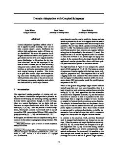
6.8 Meaning of eigenvoices Intuitively, each eigenvoice represents a characteristic of the speaker. Figure 6.10 shows the eigenvalues of the rst 30 set of Isolet (see experiments). The illustration shows the 5 rst dimensions.
Figure 6.10 Samples eigenvalues for 30 speakers E=1
50 0 −50
0
5
10
15
20
25
30
35
0
5
10
15
20
25
30
35
0
5
10
15
20
25
30
35
0
5
10
15
20
25
30
35
0
5
10
15
20
25
30
35
E=2
50 0 −50
E=3
50 0 −50
E=4
20 0 −20
E=5
20 0 −20
CHAPTER 6. EIGENVOICES
43
As we can see, the 15 rst speakers all have negative values for the rst dimension while the 15 remaining speakers all have positive values. As it turns out, the 15 rst speakers are females. The other 15 speakers are male. This property | negative values for females and positive for males | is also found throughout the whole database, with only 2{3 cross-gender errors. Therefore, we see that PCA has, by itself, identi ed the gender as the source of largest variability. The actual parameter that may be identi ed here is probably vocal tract length. Figure 6.11 shows eigenvoice 1 (representing gender) for each state. It is di�cult to mathematically trace the e�ect of the vocal tract length into PLP coe�cients.
Figure 6.11 Output EigenMeans for each states of rst eigenvoice, model part 0.04
0.04
0.02
0.02 State 2
State 1
of letter `a'
0 −0.02 0
5
10
15
−0.04
20
0.04
0.04
0.02
0.02 State 4
State 3
−0.04
0 −0.02 −0.04
5
10
15
20
0
5
10
15
20
0
5
10
15
20
0
0
5
10
15
−0.04
20
0.04
0.04
0.02
0.02
0 −0.02 −0.04
0
−0.02
State 6
State 5
0 −0.02
0 −0.02
0
5
10
15
20
−0.04
Higher order dimensions, however, are more di�cult to interpret. We have tried two approaches: 1. Given the available information on the data set, identify correlations with the eigenvalues. E.g.: given the gender of a speaker, do we know anything about the eigenvalues? 2. Given the eigenvalues, can we infer subjective knowledge about the speaker? We have three types of information for each speaker: gender, age, and origin. In gure 6.12, the last row represents the age of the speaker. We have sorted speakers in increasing age. Each other row represents the corresponding eigenvalue for each dimension. The rst dimension is clearly unrelated (there is no relationship between gender and age of enrolled speakers in the database).
CHAPTER 6. EIGENVOICES
44
For the other dimensions, it is hard to nd a relationship. Origin is not shown but it is also hard to recognize.
Figure 6.12 Age and eigenvoices 50 0 −50 0 50
5
10
15
20
25
30
35
5
10
15
20
25
30
35
5
10
15
20
25
30
35
5
10
15
20
25
30
35
5
10
15
20
25
30
35
5
10
15
20
25
30
35
0 −50 0 20 0 −20 0 20 0 −20 0 50 0 −50 0 100 50 0
0
For the second approach, we had linguists (Nancy Niedzielski, Ken Field and Steven Fincke) listen to the speech samples and interpret dimensions 2 and 3. Roughly, for dimension 2, they found � Loudness: a negative value means loud, a positive value means soft. Eigenvoice is associated to quietness. � Duration: a negative value means quick, at higher relative pitch. The results are more complicated for dimension 3. Eigenvoice may possibly be associated with duration of steady-state portion of the vowels.
Chapter 7
Experiments 7.1 Introduction This chapter contains results of the experiments that we performed to test the adaptation methods. First, we describe the problem. Then, we present the databases that were used. We explain the di�erent tests we tried with their results.
7.2 Problem We wish to increase the accuracy of recognition of utterances of letters of the alphabet. The adaptation set consists of at most a full utterance of the alphabet. We use word-models for letters. The adaptation is done in a supervised mode. We use all the available data as the observation before adapting and hence we are performing o�ine adaptation. Recognition of spelled letters is useful for reverse directory phonebooks, repair dialogues, introducing new words to the recognizer, etc. For the features, the concatenation of 8 PLP-cepstral parameters, energy, and �-cepstral coe�cients, resulting in an 18-dimensional observation vector was used.
7.3 Databases We used three databases, corresponding to an increasing level in di�culty: � Isolet: isolated, high quality, clean speech � LibStr: continuous, moderate quality, clean speech � Carnav: continuous, low quality, speech in car noise environment 45
CHAPTER 7. EXPERIMENTS
46
7.3.1 Isolet The problem
The adaptation set consists of a full utterance of the alphabet. All letters are pronounced in isolation. The test set is another utterance of the alphabet by the same speaker and in the same recording environment. Thus, both of the test set and the adaptation set are balanced1, and both are also insu�ciently representative realizations. For the decoding grammar, we use a simple loop grammar.
The sound les
ISOLET is a database recorded by the Oregon Graduate Institute (see [RACF94, RACJ96]). It consists of utterances of the English alphabet spoken in isolation. There are 150 speakers, 75 females and 75 males, all native American speakers, ages ranging from 14 to 72. Each of them pronounced the alphabet twice. Aberrations (e.g. speech uttered too soon) were discarded. The letters were then automatically extracted and manually reviewed. The recording quality is considered as high. The database is divided into ve subsets, each of which contain both utterances of the alphabet by 15 males and 15 females. Except for the distinction of sex, the subsets are arbitrarily organized. For more information on the database and how to order it, please consult [RACF94].
The speaker-independent model
We used four sets (totalling 120 speakers) to train the speaker-independent model. We used all permutations due to the sets so that we ended up with ve SI models. We have 27 models, namely one silence and all letters of the alphabet. Each model has eight states and an output probability which comprises of 6 mixture gaussians. No states, transitions or mixtures were tied. The system was trained with one gaussian mixture, then each mixture was split in two, the system was retrained, and then the number of mixtures was tripled and a nal retraining took place. An average of around 87.2% in recognition rate was achieved, which corresponds to 12.8% word-error.
7.3.2 Library StreetNames
Library StreetNames, or LibStr for short, was recorded in STL's library. It consists of 19 speakers, males, females, native and non-native speakers alike. For each speaker, we have 1 In fact, the silence model appears in each utterance, but since the recording conditions were identical, this does not in uence the results
CHAPTER 7. EXPERIMENTS
47
� a full utterance of the alphabet, in ve parts: (a,b,c,d,e,f) { (g,h,i,j,k,l) {
(m,n,o,p,q,r) { (s,t,u,v,w) { (x,y,z). The average duration of an utterance is 5 seconds. We use this part as the adaptation dataset. � utterances of 150 spelled street names. No special symbols such as `-' were used. There is no noise in the data. The speaker-independent model was trained on the OGI database: there is a mismatch between the training and testing sets. We decode with a bigram grammar.
7.3.3 Carnav
This database is almost the same as the previous one, except that utterances were pronounced in a noisy environment (in a car). The same SI models, and decoding grammar were used. We turn on the noise reduction to perform the adaptation and recognition.
7.4 Goals In this section, we review the points that we wanted to clarify with experiments.
7.4.1 Viterbi vs Baum-Welch
We want to know whether it is practical to use Viterbi state occupation probabilities instead of the optimal Baum-Welch formulae. This is motivated by the fact that practical systems use adaptation within the recognizing system. The recognizer implements Viterbi decoding and therefore yields Viterbi accumulators. We want to know what is the impact of using the Viterbi approximation.
7.4.2 MLLR Classes
Extensive research was conducted on the problem of which regression classes in MLLR [Gal96]. We want to know if using complex schemes for the generation and use of these classes ts in our interests. MLLR was implemented as a modi cation of the forward-backward algorithm. We also have it in the decoder. We used four variants � one regression class: global matrix that modi es all means � per-letter regression classes: there is one matrix per model � big clusters: we used the following clusters (built from phonetic knowledge) 1. An E-set which included the letters [b, c, d, e, g, p t, v, z]
CHAPTER 7. EXPERIMENTS
48
Figure 7.1 A tree representation of the clusters Global W
sil
E
plosive rem E E
Big clusters A-x
A
I
rem A
o
r
w
Small clusters
2. An A-set which included [a, f, h, j, k, l, m, n, s, x] 3. An I-set which included [i q u y] 4. A miscellaneous set which included [o, r, w] and was updated using a global matrix 5. A silence set which included the silence only � small clusters: we used the same clusters except that A- and E-sets were divided in two 1. A plosive E-set which included the letters [b, d, g, p t] 2. The remainder of the E-set which included the letters [c, e, v, z] 3. An A-x set which included [f, l, m, n, s, x] 4. The remainder of the A-set [a, h, j, k] Figure 7.1 shows the classes represented as a tree structure.
7.4.3 Number of iterations
In the practical system, remember that we do not want to have more than one iteration because it would mean: 1. storing the prior mean for MAPjSI 2. each new iteration costs as much as a new adaptation 3. storing the parameterized observation
CHAPTER 7. EXPERIMENTS
49
7.4.4 Number of dimensions
Eigenvoices-derived techniques assume that dimensionality of the inter-speaker variability space (eigenspace) is known a priori. Carreira-Perpinan [CP96] suggests that it is of the order of six, but has no reference to back up his hypothesis. Dimension of the eigenspace is a crucial issue in that increasing it means increasing complexity and memory use at run time, and also an increased number of speaker to obtain a reliable estimate of the eigenspace. Therefore, we want to know what is the real dimensionality, and how recognition is a�ected by reducing the number of eigenvoices. The more we reduce, the more chances we model \pure" inter-speaker variability. The more dimensions we add in, the more chances we also add intra-speaker variability-tainted eigenvoices.
7.4.5 Sparse adaptation data
As underlined in the abstract, some applications need to update a large number of parameters with very little training data. For instance, we have very short dialogues and large-vocabulary in airplane ticket reservation systems. We need to discover the minimum amount of data that we need before adaptation becomes usable. Also, we need to know which kind of data we need: in some systems we use what we have ad hoc, in others we can choose what we want the user to say and fully represent the phonetic spectrum. Therefore, studying scarcity of data in the balanced and unbalanced problems is useful.
7.5 Results
7.5.1 Results on Isolet
MLLR transformation matrices
Figure 7.2 shows the squared module of the elements of a typical matrix. Roughly, it is 3 2 .. diagonal . large 7 6 � � � 75 W = 64 � � � � (7.1) .. nil . nondiagonal and the bias vector is very small. We are using PLP-feature vectors, so that 2
static
3
7 � = 64 PLP ::: 5 6
�
7
(7.2)
CHAPTER 7. EXPERIMENTS
50
Figure 7.2 The transformation matrix (squared module)
15
10
5
0 0 5 20
10
15 10
15 20
5 0
CHAPTER 7. EXPERIMENTS
51
which means we can identify the in uence of each parameter set of the adaptation matrix 3 2 2 . 2 3 3 PLP 6PLP PLP .. � PLP7 PLP �^ = 4 : : : 5 = 64 � � � � � � � 75 4 : : : 5 (7.3) .. � � PLP � . � � Thus 2
6PLP 6 4
���
PLP
. PLP .. � �
�
.. .
�
3
PLP7
���
�
7 5
2
.. 6diagonal .
= 64 � � � nil
�
large
���
3 7 7 5
.. . nondiagonal
(7.4)
which can be explained case-by-case PLP PLP PLP parameters are orthogonal, one parameter should not a�ect another one � � Acceleration parameters might not be orthogonal � PLP Acceleration parameters carry much more information about the speaker. For instance, they are more robust to noise than static parameters PLP � same explanation
Recognition results for 6 Gaussians
The di�erent variants yielded the following results on Isolet: Variant Error rate Rel impr impr degr even � (better) � (worse) No adaptation 12.8% 0% 0 0 150 N/A N/A Global 9.9% 23% 79 27 44 4.1 1.7 Big clusters 9.3% 27% 87 28 35 4.0 2.2 Per-letter 11.6% 9% 64 51 35 4.3 2.0 MAP j SI 9.2% 28% 89 22 39 4.1 2.2 MAPjMLLR G 7.5% 41% 98 20 32 4.1 1.2 MAPjMLLR BC 7.7% 40% 101 22 27 4.0 1.5 The columns results are computed as follows: # wrong letters � Error rate: number of letters Adapted error rate � Rel impr: SI error rate SI error rate � impr: number of speakers where the number of correct answers increased. This is the cumulated results on the 5 di�erent training test splits (each with 120 speakers to train the SI and 30 to test) � degr: number of speakers where the number of incorrect answers increased. Cumulated results on the 5 di�erent test training test splits. � even: number of speakers where the number of correct answers did not change. Cumulated results on the 5 di�erent test training test splits.
CHAPTER 7. EXPERIMENTS
52
� � (better): average number of incorrectly recognized letters using SI to
decode the test alphabet for models where adaptation improved the model � � (worse): average number of incorrectly recognized letters using SI to decode the test alphabet for models where adaptation degraded the model's performance In other words � MAP using MLLR as prior yields the best results � For two thirds of the speakers we observed improvements � Error rate drops from 12.8% to 7.5%, so there is roughly a 40% relative performance improvement.
Heuristic parameters
Now we compare how methods compare with di�erent values of the parameter: we want to know whether we are sensitive to the heuristic parameter or not. Method MAPjSI MAPj MLLR G MAPj MLLR C MAPj MLLR L
� = 10 � = 20 � !1 89.82 90.33 90.82 % 87.21 % (SI) 91.49 % 92.10 % 92.49 % 90.10 % 90.44 % 90.67 % 92.33 % 90.67 % 88.08 % 88.38 % 88.62 % 88.41 % � =5
Table 7.1: Recognition Rates for Di�erent Values of �
7.5.2 Results on the LibStr database Number of iterations
From this experiment, we show that using one iteration is a good idea in practice: it only degrade performance negligibly. We used the Library StreetNames database. Of course, we used the decoder adaptation (Viterbi mode). Tables 7.2, 7.3, 7.4, 7.5 contain the recognition results for each speaker.
The heuristic parameter
In adaptation techniques where we use parameter smoothing (MAP and Viterbi retraining), the weight given to the starting point is usually xed a priori. We have conducted experiments on the libstr dataset to investigate the in uence of the value of the parameter on recognition results. Table 7.6 summarizes the results. For di�erent values of the parameter, we show the overall recognition rate. We can see that setting the parameter to a reasonable but not optimized value is acceptable. Particularly, tweaking MAPjMLLR does not help much.
CHAPTER 7. EXPERIMENTS
Spk e fw jcj kh klf mba mc mg mk nk pm pr rb rd rk scf sd tha yz Glob
SI 1 iteration 2 iterations 62.11% 64.08% 65.42% 67.65% 67.47% 67.74% 60.34% 65.65% 64.71% 69.28% 70.74% 70.74% 70.58% 73.31% 73.59% 58.95% 66.14% 65.96% 62.20% 67.40% 67.58% 75.68% 78.42% 78.14% 75.50% 78.92% 78.63% 48.11% 50.45% 50.36% 63.46% 69.90% 70.17% 55.86% 71.15% 71.15% 78.96% 78.38% 77.80% 69.91% 80.81% 82.06% 74.75% 81.63% 81.99% 75.63% 77.86% 77.67% 85.33% 87.09% 87.19% 75.70% 76.28% 76.37% 61.69% 71.69% 72.54% 67.87% 72.38% 72.52%
Table 7.2: Viterbi retraining and deleted interpolation
53
CHAPTER 7. EXPERIMENTS
Spk e fw jcj kh klf mba mc mg mk nk pm pr rb rd rk scf sd tha yz Glob
SI 1 iteration 2 iterations 62.11% 64.25% 65.42% 67.65% 67.20% 66.58% 60.34% 65.46% 66.03% 69.28% 71.01% 71.10% 70.58% 72.84% 73.50% 58.95% 66.42% 66.70% 62.20% 65.02% 67.40% 75.68% 76.87% 78.32% 75.50% 76.73% 78.63% 48.11% 51.08% 49.82% 63.46% 68.40% 68.49% 55.86% 68.44% 72.22% 78.96% 79.15% 77.70% 69.91% 77.92% 81.97% 74.75% 78.91% 80.63% 75.63% 77.12% 77.77% 85.33% 85.98% 85.79% 75.70% 75.51% 75.41% 61.69% 70.00% 70.93% 67.87% 71.38% 72.22% Table 7.3: MAP using SI priors
54
CHAPTER 7. EXPERIMENTS
Spk e fw jcj kh klf mba mc mg mk nk pm pr rb rd rk scf sd tha yz Glob
SI 1 iteration 2 iterations 62.11% 69.17% 72.39% 67.65% 73.84% 73.66% 60.34% 72.96% 72.01% 69.28% 70.83% 71.29% 70.58% 76.32% 74.91% 58.95% 69.19% 68.82% 62.20% 68.46% 69.07% 75.68% 82.60% 81.88% 75.50% 81.58% 83.10% 48.11% 51.89% 51.53% 63.46% 72.20% 70.96% 55.86% 74.35% 74.64% 78.96% 81.85% 81.95% 69.91% 82.26% 83.32% 74.75% 83.17% 83.53% 75.63% 84.93% 83.07% 85.33% 90.44% 91.09% 75.70% 80.04% 79.27% 61.69% 78.47% 79.41% 67.87% 75.92% 76.00%
Table 7.4: MAP using MLLR priors
55
CHAPTER 7. EXPERIMENTS
Spk e fw jcj kh klf mba mc mg mk nk pm pr rb rd rk scf sd tha yz Glob
SI 1 iteration 2 iterations 62.11% 68.45% 68.01% 67.65% 73.12% 74.82% 60.34% 71.44% 70.21% 69.28% 70.01% 68.73% 70.58% 76.13% 74.34% 58.95% 66.97% 67.90% 62.20% 66.78% 68.37% 75.68% 82.51% 80.05% 75.50% 81.39% 80.91% 48.11% 51.62% 33.39% 63.46% 70.79% 71.93% 55.86% 71.93% 71.54% 78.96% 81.85% 82.53% 69.91% 80.71% 81.97% 74.75% 82.71% 70.68% 75.63% 83.91% 81.40% 85.33% 90.25% 90.71% 75.70% 79.46% 75.22% 61.69% 76.27% 78.14% 67.87% 74.96% 73.09% Table 7.5: Vanilla MLLR
56
CHAPTER 7. EXPERIMENTS
57
Since this is usually the preferred adaptation method, we realize that usually we do not have to bother about adjusting the parameter. MAP � = 5 72.31 % � = 10 71.83 % � = 20 70.01 % VitRetrain � = :5 72.06 % � = :79 72.38 % � = :9 71.40 % MAPjMLLR � = 5 76.29 % � = 10 76.21 % � = 20 75.91 % Table 7.6: Tweaking the heuristic parameter for LibStr
7.5.3 Noisy environment
In this experiment, we apply the adaptation in a realistic environment. The adaptation utterances are pronounced in a noiseless, clean environment. The test set was recorded while in a car environment. We use a spectral-substraction based noise reduction technique. Table 7.7 summarizes the results. For each row, we have a speaker, and the results corresponding to each adaptation method, namely � SI: no adaptation. This is the baseline system. � Vit: with Viterbi retraining and deleted interpolation � MAP: the maximum a posteriori approach using SI as prior mean. Two di�erent values of the heuristic parameter are shown. Normal means � = 20. Unconservative means � = 5, a heavy reliance on observed data. � MLLR: the MLLR method with no MAP re nement. � MAPjMLLR: MAP using MLLR adapted model as prior mean � Multistyle: we added car noise to the temporal speech signal at di�erent levels, and recomputed the accumulators. This applies to all but the last column. � No addnoise: adapting on clean speech, without noisy \retraining". The last row, Glob, shows the average recognition rate. Viterbi-retraining combined with deleted interpolation and MAP yield similar results: where Viterbi retraining fails, MAP also fails. Using MLLR as a prior for MAP is the best combination.
7.5.4 Eigenvoices results
In this subsection, we present the results obtained with eigenvoices. We used Isolet as the database. The speaker-independent model had 6 states, and one gaussian per mixture for all states.
CHAPTER 7. EXPERIMENTS
SI
58
Multistyle No addnoise MAP MAP MLLR Spk Normal Unconservative only MAP j MLLR MAP j MLLR tha 62 % 68 % 68 % 67 % 67 % 72 % 61 % fmw 62 % 61 % 61 % 57 % 63 % 66 % 66 % ler 65 % 75 % 78 % 76 % 76 % 77 % 69 % rcb 70 % 73 % 71 % 69 % 73 % 74 % 73 % scf 74 % 78 % 77 % 75 % 84 % 86 % 69 % mig 70 % 78 % 77 % 77 % 83 % 82 % 73 % klf 70 % 74 % 76 % 73 % 77 % 76 % 72 % ssd 86 % 85 % 84 % 86 % 88 % 87 % 83 % lcy 54 % 64 % 65 % 65 % 63 % 68 % 60 % mba 55 % 58 % 58 % 61 % 66 % 68 % 58 % gjg 81 % 84 % 85 % 86 % 79 % 81 % 79 % phm 73 % 76 % 76 % 74 % 76 % 79 % 77 % jac 75 % 76 % 73 % 69 % 81 % 83 % 77 % phg 60 % 75 % 72 % 69 % 72 % 72 % 69 % msc 53 % 55 % 56 % 59 % 64 % 64 % 60 % yiz 61 % 69 % 70 % 74 % 63 % 68 % 64 % nan 67 % 67 % 67 % 67 % 67 % 69 % 66 % rls 62 % 67 % 63 % 63 % 72 % 68 % 61 % jmc 73 % 74 % 70 % 67 % 73 % 75 % 74 % rjz 80 % 85 % 81 % 80 % 85 % 87 % 85 % Glob 67.55% 72.15% 71.35% 70.70% 73.60% 75.08% 69.71% Vit
Table 7.7: Adaptation in a realistic environment
CHAPTER 7. EXPERIMENTS
59
Figure 7.3 The estimate of variance of the coordinate decreases with the dimension
600
Test set Training set 500
Estimated variance
400
300
200
100
0
1
2
3
4
5 6 Dimension #
7
8
9
10
Number of dimensions
For eigenvoice techniques, we have to answer the following question: what is the minimum intrinsic dimensionality of the speaker space? In other words, how many parameters do we need to estimate to have an accurate model? If we estimate too many dimensions, then we may catch intra-speaker variabilities. When the dimensionality reaches in nity, it is easy to show that lim � = �ML (7.5) E !1 MLED
we converge to the maximum-likelihood estimation. If we have too few dimensions, on the other hand, the constraint is too strong. By construction, when using PCA, dimension k + 1 is estimated from the residual errors of dimension k. Figure 7.3 shows the estimated variance. Due to PCA's ordering, the smaller dimensions accumulate the largest variances. variability is larger than intra-speaker variability. Figure 7.4 shows the relative error for each dimension: q X (we(test) we(ref)) (7.6) Relative error = jwe(ref)j speakers Figure EvsER shows recognition results as a function of the dimensionlity of the eigenspace. Using MAP after MLED is very helpful since the recognition
CHAPTER 7. EXPERIMENTS
60
Figure 7.4 Normalized Euclidean distance 0.35
0.3
Relative error
0.25
0.2
0.15
0.1
0.05
0
1
2
3
4
5 6 Dimension #
7
8
9
10
Figure 7.5 Choosing the dimensionality of the eigenspace Impact of dimension of eigenspace on recognition rate 90
89
Recognition rate
88
87
86
85
84
MLED MAP|MLED, τ = 10 MAP|MLED, τ = 20 MAP|MLED, τ = 40 0
5
10
15 Dimension of eigenspace
20
25
30
CHAPTER 7. EXPERIMENTS
61
rate becomes almost constant. When the dimensionality is small, then MLED imposes very strict constraints and the recognition results su�er, and when we add dimensions we nd a better estimate. After E = 10, the eigenvalues become small and have a low impact on recognition results.
Sparse adaptation data
The most interesting case for MLED is where we have a very small amount of adaptation data. We show that MLED performs considerably better than MLLR, MAP or any combination those of. As underlined in the introduction (see 2.2), there are two di�erent phenomena occurring when we lack enough data. Table 7.8 shows recognition results for the methods when we have balanced missing data: we have removed 9 letters, � 4 letters from the A-set: A, H, K, L. � 4 letters from the E-set: B, E, P, T. � 1 letter not belonging to the previous sets: O. Method Recognition Results MAPj MLLR G 82.87 % MAPj SI 82 % MLED (E=10) 87.54 % SI 81.2 % Table 7.8: Recognition Rates with balanced missing data We now make the problem harder for MLLR: we remove all 9 letters of the E set (B, C, D, E, G, P, T, V, Z). Table 7.9 summarizes the results. Method Recognition Results MAPj MLLR G 81.08 % MAPj SI 84.69 % MLED (E=10) 86.51 % SI 81.2 % Table 7.9: Recognition Rates for unbalanced adaptation data With almost no adaptation data, standard adaptation techniques just yield unusable estimates. This time, we compare MLED with di�erent dimension of the eigenspace. Table 7.10 shows the results. We used letters A, B, C, and U to adapt the model. For minimal adaptation data, we observe that, surprisingly, MLED still works. Table 7.11 shows adapting still helps. We use only one letter to adapt
CHAPTER 7. EXPERIMENTS
62
Dimension Recognition Results E=1 85.13 % E=5 86.36 % E=10 86.61 % SI 81.2 % Table 7.10: Adapting with a small amount of data with. We tried with two letters of the alphabet, A, and S. As the dimension increases, error rate also increases, but we can still estimate the few rst eigenvalues quite accurately. Adapting with `A' is easier because it is a vowel. We are able to guess the rst dimension (sex) quite accurately. Dimension E=1 E=5 E=10 SI
Letter A 84.97 % 85.67 % 83.69 % 81.2 %
Letter S 85.08 % 84.38 % 82.64 % 81.2 %
Table 7.11: Adapting with one letter To summarize, gure 7.6 shows the learning curve for MLED using 1, 5, and 10 dimension. While being a popular measure, learning curves are not meaningful per se as long as we do not specify if the data is balanced. For this graph, we used � A for one adaptation utterance � A,B,C,U for four utterances � (C, D, F, G, I, J, M, N, Q, R, S, U, V, W, X, Y, Z) for seventeen utterances � the full alphabet for 26 utterances
7.6 Summary In short, we can conclude that � it is always better to use MAPjMLLR rather than MLLR only. � it is best to use MAPjMLLR with one global matrix � we are relatively insensitive to heuristic parameters � using Viterbi instead of Baum-Welch does not hurt
CHAPTER 7. EXPERIMENTS
63
Figure 7.6 Learning curve: error rate vs number of adaptation utterances 88
87.5
87
86.5
86
85.5
85
84.5
E=1 E=5 E = 10
84
83.5
0
5
10
15
20
25
30
� there is little advantage in using MAPjSI rather than the current (opti� � � �
mized) Viterbi-based adaptation it is safe to truncate the EM-algorithm to the rst iteration MLED performs very well when adaptation data becomes scarce the number of dimensions we should use depends on the amount of adaptation data using speaker adaptation, one can expect approximately 20 % to 40 % relative improvement in the error rate.
Chapter 8
Conclusion In this chapter, we explain in short what has been accomplished during my internship. We start by stating our objectives for the internship, and how they have been met. Then, we summarize the results and theoretical developments that constitute the core of this report. Lastly, we envision further research in the area.
8.1 Goals and achievements For the Eur�ecom industrial thesis, we have to meet two requirements: 1. academic relevance: the student has to demonstrate mastery of concepts acquired during his training and ability to learn new theoretical concepts. In our case, the goal was to understand MLLR and MAP. 2. industrial relevance: the student has to prove usefulness to the enterprise by developing actual, relevant material. In our case, it consisted of implementing MLLR and MAP. I have achieved the following points: 1. academic relevance: a new method, based on eigenvoice, was developed. Its mathematical formulation was completed. Variants and improvements were invented. It showed considerable improvement for sparse data. Adaptation methods were theoretically compared. I am co-author of two publication submissions. 2. industrial relevance: three US patent applications were submitted. MLED, MLLR and MAP were implemented, tested, and compared. A combination of these (MAPjMLED and MAPjMLLR) was devised, and generated considerable improvements. A practical, useable implementation was realized. 64
CHAPTER 8. CONCLUSION
65
8.2 Summary Throughout this internship, I worked on speaker adaptation. I de ned a set of properties to compare adaptation techniques formally. Two popular adaptation techniques, MLLR and MAP, were implemented. At this point we were able to reproduce experiments from the state-of-the-art literature, as a baseline for comparison. Then, a combination of MLLR and MAP was implemented, increasing performance by almost one third. Furthermore, a new adaptation technique that applies the ML criterion to eigenvoices was designed and tested. Very promising results in the case of sparse adaptation data were obtained. It is hoped that research on the eigenvoices idea will continue.
8.3 Future Work Compared to MLLR and MAP, eigenvoices is still immature. It has not been publicly presented yet. Thus, the research community did not have a chance to work on it yet, as opposed to other adaptation techniques. Yet, very competitive results have been observed. Therefore, it is felt that future work should focus on eigenvoices. Moreover, since our estimate depends strongly on the eigenspace, one should explore: � experimenting on medium- to large-vocabulary systems � estimation of the eigenspace using realistic size of databases. � the unbalancedness with respect to speaker-variety in the training set of speakers should be considered. � guiding the eigenspace-discovery algorithm (eg with LDA) might prove useful � the ability of eigenvoices to work on environmental variety should be tested and explored as well. � for dictation systems, we should derive a method for transposing the eigenspace to unknown test conditions (eg user's o�ce environment). In telephone-based systems, quality (mobile, speaker-phone, pay phone, etc) and background noise are sources of variability. � databases that catch all these variabilities should be constructed.
Appendix A
Mathematical derivations A.1 Expectation-Maximization Algorithm The objective we are striving for is that of optimizing the likelihood of an observation L(Oj�) by changing the model parameters. We showed how to compute this likelihood given a model in the introduction 1.3. Due to the hidden nature of the process (see gure A.1), there exists no su�cient statistics of xed dimension for the model parameters: given the observation vectors, we do not know for how much time the HMM stayed in each state and which mixture gaussian was used to produce the vector.
Figure A.1 Hidden Markov Process
?
?
?
?
?
?
?
observation frames
There is no known algorithm to solve the problem of optimizing the model � given the observation only. This problem is called the incomplete data problem because we do not know the state sequence / mixture component sequence that produced the realization. To solve this issue, we complete our data by estimating missing data with our current t. Using our new solution, we re ne 66
APPENDIX A. MATHEMATICAL DERIVATIONS
67
our estimation of missing data and apply the procedure again with a new, better t. In the next subsection, we present a sketch of the corresponding mathematical development.
A.1.1 Mathematical formulation
We start o� with our current t �^, the model that we re ne. We also have O, the observed data. The incomplete data problem is
O ! (�; � ); max L(Oj�) � With � the state and mixture component sequences provided by the optimal model. We approximate these with the ones provided by �^, to solve the (easier) complete data problem:
O; (�; � ) ! max L(Oj�) � D = (O; �; � ) is all we need to solve the problem and hence is referred to as
complete data. Since we are unsure of our state-mixture component sequence, it is wise to maximize the expectation of the function given �^ and the observation h
Q(�; �^) = E log L(O; �; � j�)jO; �^ If we let
h
i
H (�; �^) = E log L(O; �; � jO; �)jO; �^
(A.1) i
(A.2)
and observe that log L(Oj�) = Q(�; �^) H (�; �^) Jensen's inequality is applied on H (�; �^), h
i
H (�^ ; �^) = E log L(O; �; � jO; �^)jO; �^ � H (�; �^)
(A.3) (A.4)
and therefore increasing Q(�; �^) also increases log L(Oj�). The expectation given the model is obtained through summation over all possible state and mixture sequences, X X Q(�; �^) = L(O; �; � j�) log L(O; �; �j�^ ) (A.5) �2� � 2 � This is called the expectation step (E-step).
APPENDIX A. MATHEMATICAL DERIVATIONS
68
For HMMs, the likelihood of the completed data is
L(O; �; � j�) = a�T N
T Y t=1
a�t 1 �t c�(�t t ) b�(�t t ) (ot )
(A.6)
We can replace this expression in the previous formula. Maximization satis es
@Q = 0 @�
(A.7)
This is the maximization step (M-step).
A.1.2 Extension of the algorithm to MAP
In the MAP case, we want to optimize (using Bayes' rule) log f (�jO) = log f (Oj�) + log P0 (�) (A.8) A little thought convinces us that with log f (�jO) = Q(�; �^) H (�; �^) + log P0 (�) (A.9) rede nition of the auxiliary function as R(�; �^) = Q(�; �^) + log P0 (�) (A.10) is su�cient to generalize the EM-algorithm to the MAP optimization criterion.
A.2
Q-function
factorization
As stated in section 3.2, we need to optimize X Q(�; �^) = L(O; �j�) log L(O; �j�^ ) �2� with � = (�1 ; :::; �T ) a state sequence, and � the set of all possible state sequences for that observation. If we consider each mixture component m as a parallel branch in the state sequence, we are able to decompose the auxiliary function into X X L(O; �; � j�) log L(O; �; �j�^ ) (A.11) Q(�; �^) = �2� � 2 � with similarly � = (�1 ; :::; �T ) a mixture component sequence and � the set of all possible mixture component sequences given �. The likelihood will then be
L(O; �; � j�) = a�T N
T Y t=1
a�t 1 �t c�(�t t ) b�(�t t ) (ot )
(A.12)
APPENDIX A. MATHEMATICAL DERIVATIONS
69
Substituting the last formula into the Q function, we get
Q(�; �^) =
X X
�2� � 2 �
(
L(O; �; � j�) log a^�T N +
X
t
log a^�t 1 �t +
X
t
)
X log c^�(�t t ) log ^b�(�t t ) (ot )
t
(A.13) We are only interested in means update, so that c^ = c and a^ = a, and we can write Q(�; �^) = Qa (�; faij g) + Qb (�; ^b(ms) ) + Qc (�; fc(ms) g) (A.14) with X X X Qb (�; ^b(ms) ) = L(O; �; � j�) L(O; �t = s; �t = mj�) log ^b(ms) (ot ) t �2� � 2 � (A.15) and Qa , Qb constant. De ning the mixture component occupation probability and the state occupation probability as respectively XX L(O; �t = s; �t = mj�) (A.16)
m(s) (t) = L(O1 j�) � � (s) (s) (A.17) = (s) (t) P cm b(ms) ((os)t ) ( o ) b c r r t r 2s X 1 ( s )
(t) = L(Oj�) L(O; �t = sj�) (A.18) � So we can conclude that the function we need to optimize is X Qb (�; ^b(ms) ) = L(Oj�) m(s) (t) log ^b(ms) (ot ) = L(Oj�)
t
X
t
(A.19)
� �
m(s) (t) n log(2�) log jCm(s) j + (ot �^(ms) )T Cm(s) 1 (ot �^(ms) )
(A.20)
A.3 Maximizing Q with W From section A.2, we have derived the formula of the function we need to optimize: XXX
m(s) (t)[n log(2�) + log jCm(s) j + h(ms) (ot ) Q = 21 L(Oj�) s m t where h(ms) (ot ; s) = (ot �^(ms) )T Cm(s) 1 (ot �^(ms) )
APPENDIX A. MATHEMATICAL DERIVATIONS
70
Having completed the mathematics for the means likelihood computations in the HMM case (see section 3.2), we now want to optimize this function with an a�ne transformation as explained in section 4.1, eq. 4.1. To achieve this, we di�erentiate Q @Q = 1 L(Oj�) X X X (s) (t) @ h(s) (o ) (A.21) m @W m t @W 2 s m t Since
2
3
.. (s)T T (s) 1 4 � 1� � 5 ( s ) T ( s ) 1 hm (ot ) = ot Cm ot + [1 . �m ]W Cm W (s) �
�m
. (s)T T (s) 1 � 2[1 .. �m ]W Cm ot the following holds:
�
@ h(s) (o ) = [1 ... �(s)T ] @ W T C (s) 1 W m m @W m t @W
�
(A.22)
. (s)T (s) 1 @ T [1 .. �m ]Cm @W W ot (A.23)
@Q to zero and replacing the di�erentiation, we get Equating @W 2
3
@Q = 0 = X X X (s) (t)C (s) 1 (o W 4 � 1� � 5)[1 ... �(s)T ] t m m m @W s m t �(ms) and hence we state
2
(A.24)
1
XXX 6 .
m(s) (t)Cm(s) 1 ot [1 .. �m(s)T ] =
m(s) (t)Cm(s) 1 W 64 � � � s m t s m t �(ms)
XXX
now
Z=
XXX
s m t XXX
.
m(s) (t)Cm(s) 1 ot [1 .. �m(s)T ] 2
1
6
m(s) (t)Cm(s) 1 W 64 � � � s m t �(ms) Z =Y
Y=
.. .
�
.. .
�
�m(s)T
���
.. (s) (s)T . �m �m (A.25) (A.26)
�m(s)T
���
.. (s) (s)T . �m �m
3 7 7 5
(A.27)
(A.28) and let also ot [i] be the ith feature of ot , and similarly for �(ms) and �(ms) [i], Cm(s) 1 [i] be the i diagonal component of Cm(s) 1 , we have each component
3 7 7 5
APPENDIX A. MATHEMATICAL DERIVATIONS
71
zij ; i = 1:::N; j = 1:::N + 1 of the left-hand side matrix of the equation to be
zij =
P (s)
m (t)Cm(s) s m P P Pt (s) (s) s m t m (t)Cm
� P P
1 [i]ot[i]; if j = 1 1 [i]o [i]�(ms) [j 1]; else t
This is useful for understanding the algorithm. As for the right-hand side of the equation, we de ne X Vm(s) = m(s) (t)Cm(s) 1 t
2 6
.. .
1
Dm(s) = 64 � � � �(ms)
�m(s)T
�
���
(A.29)
(A.30)
3 7 7 5
.. (s) (s)T . �m �m Replacing the previous de nitions into Y , we have XX Y= Vm(s) WDm(s) s m
(A.31)
(A.32)
Since it appears that if we again assume Cm(s) 1 to be diagonal Vm(s) inherits from the same property, we can solve the equation row by row. Subsequently, P we de ne wi ; i = 1::N the ith row of W , and vi = t m(s) (t)Cm(s) 1 [i] we decompose the equation into N equations of order (N + 1) each, in other words 2
Z
6 6 XX6 6 = 6 s m 6 4
v1 w1 .. .
3 7 7 7 7 7 7 5
vi wi Dm(s) .. .
vN wN
(A.33)
Each of these subequations is described by G(i) , of elements gjq ; j = 1:::N + 1; q = 1:::N + 1 X G(i) �= gjq(i) = vi djq (A.34) m
and because the matrix is symmetric, we can nally state zi = G(i) wiT
(A.35)
which means as previously underlined, N matrix inversions to perform per each regression class.
APPENDIX A. MATHEMATICAL DERIVATIONS
72
A.4 Di�erentiation of h(ot; s) for eigenvoices
In this section, we show how to di�erentiate h(�) with respect to the eigenvalues. First of all, let us show that E @ �^(s) = @ X (s) (s) m @we @we j=1 wj �m (j ) = �m (e)
(A.36)
We have
@ h(o ; s) = @ (o �^(s) )T C (s) 1 (o �^(s) ) (A.37) t m @we t @we t m m @ noT C (s) 1 o 2oT C (s) 1 �^(s) + �^(s) C (s) 1 �^(s) o (A.38) = @w t t m m m m m e t m distributing the di�erentiation operator, we get �
�
@ �^(s) + @ ��^(s)T C (s) 1 �^(s) � = 2oTt Cm(s) 1 @w @we m m m e m
(A.39)
using eq. (A.36), and basic properties of di�erentiation, = 2oTt Cm(s) 1 �(ms) (e) +
�
�
�
@ �^(s)T C (s) 1 �^(s) + �^(s)T C (s) 1 @ �^(s) m m m m @we m @we m (A.40)
and since scalars are equal to their transpose: �
�
@ �^(s)T C (s) 1 �^(s) = 2oTt Cm(s) 1 �(ms) (e) + 2 @w m m e m
(A.41)
further application of rule eq. (A.36) yields, E
(s)T (e)Cm(s) 1 X wj �(ms) (j )] = 2[ oTt Cm(s) 1 �(ms) (e) + �m j =1 We do not require the covariance matrix to be diagonal.
(A.42)
A.4.1 Linear dependence
We can relax the assumption that the eigenvalues are orthogonal
@ w � 0; @we j
j 6= e
(A.43)
Eigenvalues can be dependent of each other wj = f (fwk g; k 6= j )
(A.44)
�
APPENDIX A. MATHEMATICAL DERIVATIONS
73
There is nothing in PCA that disallows this. We can assume the dependence is linearly separable,
f (fwk g; k 6= j ) =
X
k6=j
fk (wk )
(A.45)
in which case we just replace eq. A.36 by E @ �^(s) = @ X (s) @we m @we j=1 wj �m (j )
@ X f (w ) k k j =1;j 6=e @we k6=j � � @f ( w ) e e ( s ) = �m (e) 1 + @w e = �(ms) (e) +
X
(A.46) (A.47) (A.48)
and if fe (we ) is linear then there is no additional complexity.
A.4.2 Scaling and translation of eigenvectors
To avoid numerical instability when applying PCA, we rst nd the eigenspace modelling the residual error � ! �0 + �; �0 = E� then we scale each component by its standard deviation
� ! ��
De ning D to be the diagonal matrix of the standard deviations for each mixture mean, and P to be the matrix of eigenvectors, we update with X �^(ms) = DP [w(1) ::: w(E )] + �0 = [(D�(e)) w(e)] + �0 (A.49) e
and therefore all equations are the same except that we rst scale the eigenvectors by the standard deviation and then at update time translate by �0 .
A.5 MAP Reestimation formulae In this section, we brie y review the key points of the derivation of the MAP means update formulae. Given that we need to solve @Q + @ log P0 (�) = 0 (A.50)
@�
@�
The general solution is hard. Therefore, we will restrain P0 (�) to belong to the family of conjugate priors of O. A conjugate prior for a random variable O is a pdf for which
APPENDIX A. MATHEMATICAL DERIVATIONS
74
� there is su�cient statistics of xed dimension. Obviously, this is required
as we do not want to have to apply EM again. � the posterior distribution f (�jO) and P0 (�) belong to the same distribution family, viz
f (�jO) _ P0 (�)
(A.51)
In our case, we want
log f (�jO) = Q(�; �^) H (�; �^) + log P0 (�) _ P0 (�)
(A.52)
It has been veri ed that the conjugate prior for observation of HMMs (given the completed data) is the product of Dirichlet with normal-Wishart densities. We assume parameters of HMMs are independent: o o n n (A.53) P0 (�) = pc ( c(ms) )pm ( �(ms) ; Cm(s) ) with pc(�) the Dirichlet densities of hyperparameters (ms) : n o Y (s) pc ( c(s) ) = cm(s) m m
s;m
(A.54)
and pm (�) the said normal-Wishart density with hyperparameters �m(s) , �(0sm) , �(ms) and u(ms) , # " (s) (s) � � 1 n �T � o � m (s) (�m N )=2 ( s ) ( s ) ( s ) 1 ( s ) ( s ) ( s ) ( s ) 1 �m �0m 2 tr um Cm exp Cm 2 �m �0m Cm (A.55) We simplify for the means-only case: # " (s) � � � �T � m ( s ) ( s ) ( s ) ( s ) 1 ( s ) �m �0m P0 (�) _ exp 2 �m �0m Cm
(A.56)
It is well-known that the conjugate prior of a gaussian mean with xed covariance is also a gaussian. Replacing the prior density into our auxiliary function and solving for the mean �(ms) yields (s) + P m(s) (t)ot � m ( s ) �m = (s) Pt (s) (A.57) �m + m (t) t
Appendix B
Algorithms B.1 MLLR: Slow algorithm foreach observation O { Z[i,j] = 0; i = 1..n, j = 1..n+1 G(k)[i,j] = 0; i = 1..n, j = 1..n+1, k = 1..n+1 foreach model m iterate over time t { S = 0; /* sum of alpha-beta */ foreach state s in model S += alpha(s) . beta(s); foreach state s in model for each mixture m gamma = alpha(s) . beta(s) / S . weight(s,m) . normal(o, mu[m], var[m]) / P(O|s); foreach dimension i foreach dimension j Z[i][j] += gamma . o[i] . inverseVar(s,m)[i] . xi[j] foreach dimension k foreach dimension i foreach dimension j G(k)[i,j] += gamma . inverseVar(s,m)[k] . xi[i] . x[j]; } if baseclass is letter { store Z, G for that model Z[i,j] = 0; i = 1..n, j = 1..n+1 } else /* one matrix for all mixtures */ {} }
75
APPENDIX B. ALGORITHMS
76
B.2 MLLR: Fast algorithm (From ComputeMix.c): Build the data structures: the dictionary, the update structure (aka accumlators), etc. Foreach observation O, Modi ed forward-backward algorithm: (in libs/bwtrain.c, ComputeMLLRAccumulator): Build the treillis structure (BuildBWTrlS) Compute the distribution values for O (the b(ms) (ot )) (SmartCompDistrTrl) Compute the backward probabilities beta, using BackwardTrl Use the modi ed forward algorithm (ForwardGlobalMLLR): Foreach ot in O, make the forward step GlobalMLLRForwardStep: Foreach state TrlFrom in trellis column Foreach state in current model P complete the forward step and compute � Foreach state in current model P State likelihood = dlike (� cm bm (ot )) initialized to 0. Foreach distribution in output probability: dlike = dlike + cm bm (ot ) but in log domain Foreach mixture m inPthe output probability: P Compute = � =( � )cm bm =( cm bm ) P Compute Am [0]+ = (since Am [0] is bound to be Tt m (t)) Compute Am [1 : : : n]+ = ot [0 � � � n 1] Update the means using libs/bwtrain.c: GlobalMLLRUpdMeans: . allocate zero-initialized space for the n � (n + 1) � (n + 2) matrices ([G(i) ..ziT ]; i = 1:::n) (in the remainder, you can assert that GZt is accessed with i, j , r indices, as in GZt[i][j ][r]. allocGZt: allocate contiguous memory space (faster) Foreach model � in the dictionary (not in the trellis!), Foreach state s = 1:::S� in the model, Foreach gaussian mixture component m = 1:::Ms, ll in Z part of the GZt supermatrix: Foreach dimension i = 0:::n 1 as in G(i) (denoting the row if W ), GZt[i][0][n + 1]+ = Am [i + 1] � �m (i) (�m (i) is the ith diagonal component of the covmatrix Foreach dimension j = 0:::n 1 in ziT , Have GZt[i][j + 1][n + 1]+ = ziT (j ) = �m (i)Am [i + 1]�m(j ) ll in G part of the GZt supermatrix: Foreach dimension i = 0:::n 1 as in G(i) (denoting the row if W ), GZt[i][0][0]+ = �m (i)Am (0) Foreach dimension r = 0:::n 1 (set the rst row, iterate of the columns of that row) GZt[i][0][r + 1]+ = �m (i)Am (0)�m (r) Foreach dimension j = 0:::n 1 (now iterating on the rows of G) GZt[i][j + 1][0]+ = �m (i)Am (0)�j (set the rst column) Foreach dimension r = 0:::n 1 (now iterating on the columns of G) GZt[i][j + 1][r + 1]+ = �m (i)Am (0)�j �r Allocate (contiguous) space for n � (n + 1)-matrix W allocMatrix. Foreach dimension i = 1:::n 1 (row if W ),
APPENDIX B. ALGORITHMS
77
. solve the system de ned by GZt[i] = [G(i) ..ziT ] ((n + 1) � (n + 2) into the row W [i]. print the solution in a matlab format so we can copy-paste to check the results Foreach model � in the dictionary (not in the trellis!), Foreach state s = 1:::S� in the model, Foreach gaussian mixture component m = 1:::Mc, Foreach dimension t = 1:::n of the mean, compute X [t] = W [1...�Tm]T , X [t] = W [t][0] (which is the bias term) Foreach dimension r = 1:::n (column-1 of W ), X [t]+ = �m (r)W [t][r + 1] Foreach dimension t = 1:::n of the mean, (we are updating the mean) �^m (t) = "�m (t) + (1 ")X [t], here " = 0 Free W and GZt (super)matrices. Overwrite dictionary Free Structures and Close le Beam when either of
P
� , or N (ot ; �m ; �m ) is too small.
B.3 Current STL algorithm In this algorithm, we adapt instantaneously. We use Viterbi state occupation probabilities. We only keep track of zero-th order accumulator. We de ne the instantaneous zero-th accumulator to be
A(ms) (U ) =
U X t=1
m(s) (t) = number of frames seen for that gaussian up to time U (B.1)
with U the current frame being processed. With � our heuristic parameter, 0 � � � 1, de ne n o 5 =8 (B.2) �0 = 1 + (� 1) exp( A(ms) ) 0 �m = (1 � ) (B.3) We update the means using �^(ms) = �0 �(ms) + �m oU
(B.4)
The algorithm can thus be described as 1. Perform forced alignment (or recognition for unsupervised adaptation) 2. For the given observation, iterate over time and update the means using eq. (B.4)
APPENDIX B. ALGORITHMS
78
B.4 Cost In this section, we consider the cost of the hereinbefore presented algorithms (see B.1, B.2 and B.3). We consider cost in the computational and memory domain. Let us introduce the notation: T the average number of feature vectors in an observation, about 40 to 70 for each letter Q the number of observations, here 26 K the number of non-distinct HMMs observed in each observation, here 3 (sil Letter sil) H the number of HMMs in the model, here 27 S the number of states in each HMM, here 8 M the number of mixtures in each state, here 6 n the dimension of the observation vector, here 18 O(�) order of the cost function So, for the sake of simplicity we assume that � all observation bear the same length � all HMMs have the same number of states � all states have the same number of mixtures
B.4.1 MLLR
For the fast algorithm, we consider four nontrivial phases (see section 4.3): 1. compute the accumulators in the forward-backward algorithm: � memory use per mixture is (n + 1) � sizeof(Real), and sizeof(Real) is two machine-words. Thence, we have O(H � S � M � (n + 1) � 2). � computational cost: O(Q � T � K � S � M � (n + 1)). 2. gather the results (could be divided by two because matrices are symmetric): . � memory use for n times [G(i) .. ziT ] matrices is O(n � (n +1) � (n +2)) � computational cost: O(H � S � M � n � (n + 1) � (n + 2)) 3. nd W row by row: � memory use: O(n � (n + 1)) � computational cost: for each row, we use O((n + 1)3 ) matrices inversion, so we have O(n4 ) 4. update the means using equation 4.1 � memory use: O(n) � computational cost: O(H � S � M � n � (n + 1))
APPENDIX B. ALGORITHMS
79
Thus, for the computation, the algorithm needs O(H � S � M � n) + O(H � S � M � n � n2 ) + O(n4 ) + O(H � S � M � n2 ) � O(n4 ) (B.5) Numerically, the matrix inversions are the dominant term. For the memory use, we have O(H � S � M � n) + O(n3 ) + O(n2 ) + O(n) � O(H � S � M � n) (B.6) Numerically, the storage space needed for the accumulators (around 100 kB) is dominant.
B.4.2 MLED
For eigenvoices methods, let us de ne E as the dimension of the eigenvoice space. As with other EM-based algorithms, we proceed in three phases, namely 1. Compute the accumulators 2. Gather the resullts 3. Update the model means The computational cost and memory use for the rst step is � computations: O[Q � T � K � M (n + 1)] � memory: O[H � S � M � (n + 1)] Gathering the results and computing the eigenvalues is (without precomputation) � computations: O[E 2 � H � S � M � Q � n2 ] to compute the matrix, and O[E � H � S � M � Q � n2 ] for the vector. Inverting the matrix takes O[E 3 ].
� memory: storage space for eigenvalues, matrices to invert, and solution vector (w; V; Q): O[E + E � E � E ] = O(E 3 ). Storage space for the eigenvoices (vectors): O[H � S � M � n � E ]
To update the model means, we keep the eigenvoices and eigenvalues from the previous step. Therefore, there is no additional memory allocation here. We just multiply the eigenvalues and add up the results, and the corresponding computational cost is given by
O[E � H � S � M � n] Applying MAP adds an insigni cant number of computations, O[H � S �
M � n].
APPENDIX B. ALGORITHMS
80
Accumulators
The computational cost and memory use for the rst step is � computations: O[Q � T � K � M � (n + 1)] � storage: O[H � S � M � (n + 1)]
Gathering the results
Gathering the results and computing the eigenvalues is (without the precomputation optimization) � computations: O[E 2 � H � S � M � Q � n2 ] � storage: O[E 2 � H � S � M � Q � n2 ]
Updating the means
We keep the eigenvoices from the previous step, so there is no additional memory allocation here. We just multiply these eigenvalues and add up the results, and the corresponding computational cost is given by
O[E � H � S � M � n] Applying MAP thereafter adds an insigni cant number of computations
O[H � S � M � n]
Bibliography [ADR77] N.M. Laird A.P. Dempster and D.B. Rubin, Maximum-Likelihood from Incomplete Data via the EM algorithm, Journal of the Royal Statistical Society B (1977), 1{38. [AH98] Mohammed A fy and Jean-Paul Haton, Minimum Cross-Entropy Adaptation of Hidden Markov Models, ICASSP (1998). [AS96] Seyed M. Ahadi-Sarkani, Bayesian and Predictive Techniques for Speaker Adaptation, Ph.D. thesis, University of Cambridge, Cambridge, UK, January 1996. [Bau72] L.E. Baum, An inequality and associated maximization technique in statistical estimation for probabilistic functions of Markov processes, Inequalities 3 (1972), 1{8. [BM97] Enrico Bocchieri and Brian Mak, Subspace distribution clustering for continuous observation density Hidden Markov Models, Eurospeech 97, 1997. [BMP96] C. Nastar B. Moghaddam and A. Pentland, A Bayesian Similarity Method for Direct Image Matching, International Conference on Pattern Recognition (1996). [Cox92] S. Cox, Predictive speaker adaptation in speech recognition, Computer speech and language 9 (1992), no. 1, 357{365. [CP96] Carreira-Perpinan, A review of dimension reduction techniques, Tech. report, Department of Computer Science, University of She�eld, UK, September 1996, CS-96-09, see also http://www.dcs.shef.ac.uk/~miguel/research.html. [CW97] Jen-Tzung Chien and Hsiao-Chuan Wang, Telephone speech recognition based on Baysian adaptation of hidden Markov models, Speech Communication 22 (1997), 369{384. [Gal96] M. J. F. Gales, The Generation and Use of Regression Class Trees for MLLR Adaptation { TR.263, Tech. report, Cambridge University Engineering Department, August 1996. 81
BIBLIOGRAPHY [Gal97] [GL92] [GL94]
[GY93] [HHW85]
[JH96]
[Jol86] [Kuh97] [LW94] [LW95a] [LW95b] [NMK97]
82
M. J. F. Gales, Maximum Likelihood Linear Transformations for HMM-based Speech Recognition { TR.291, Tech. report, Cambridge University Engineering Department, May 1997. J.-L. Gauvain and C.-H. Lee, Bayesian Learning for Hidden Markov Model with Gaussian Mixture Observation of Markov Chains, Speech Communication 11 (1992), 205{213. J.-L. Gauvain and C.-H. Lee, Maximum a posteriori estimation for multivariate Gaussian mixture observations of Markov Chains, IEEE Transactions on Speech and Audio Processing 2 (1994), no. 2, 291{ 298. M.J.F. Gales and S.J. Young, Parallel model combination for speech recognition in noise, Tech. report, Oregon Graduate Institute of Science and Technology (OGI), June 1993, CUED/F-INFENG/TR 135. Brian A. Hanson Hynek Hermansky and Hisashi Wakita, LowDimensional Representation of Vowel Based on All-Pole Modelling in the Psychophysical Domain, Speech Communication 4 (1985), 181{187. Jean-Claude Junqua and Jean-Paul Haton, Robustness in Automatic Speech Recognition { Fundamentals and Applications, Kluwer Academic Publishers, Speech Technology Laboratory, Santa Barbara; CNRS, France, 1996. I. T. Jolli�e, Principal Component Analysis, Springer-Verlag, Berlin, 1986. Roland Kuhn, Eigenvoices for Speaker Adaptation, Tech. report, Speech Technology Laboratory (STL), July 1997. C. J. Leggetter and P. C. Woodland, Speaker Adaptation of HMMs using Linear Regression { TR.181, Tech. report, Cambridge University Engineering Department, June 1994. C. J. Leggetter and P. C. Woodland, Flexible speaker adaptation for large vocabulary speech recognition, ESCA { European Conference on Speech Communication and Technology 2 (1995), 1155{1158. C. J. Leggetter and P. C. Woodland, Maximum likelihood linear regression for speaker adaption of continuous density hidden Markov models, Computer Speech and Language 9 (1995), 171{185. Hynek Hermansky Narendranath Malayath and Alexander Kain, Towards decomposing the sources of variability in speech, Eurospeech (1997).
BIBLIOGRAPHY [Pat98]
83
Patrick Nguyen, Roland Kuhn and Jean-Claude Junqua, Patent Submission for a Maximum-likelihood Method For Finding An Adapted Speaker Model In Eigenvoice Space, apr 1998, Submitted on April 13, 1998. [PNBK97] Jo~ao P. Hespanha Peter N. Belhumeur and David J. Kriegman, Eigenfaces vs. Fisherfaces: Recognition Using Class Speci c Linear Projection, IEEE Transaction on Pattern Analysis and Machine Intelligence 19 (97), no. 17, 711{730. [RACF94] Yeshwant Muthusamy Ronald A. Cole and Mark Fanty, The ISOLET Spoken Letter Database, Tech. report, Oregon Graduate Institute of Science and Technology (OGI), 19600 N.W. von Neumann Drive, Beaverton, OR 97006, November 1994, available as http://www.cse.ogi.edu/CSLU/corpora/isolet.html. [RACJ96] Murali Gopalakrishnan Ronald A. Cole, Mark Fanty and Rik D.T. Jansen, Speaker-independent name retrieval from spellings using a database of 50,000 names, IEEE S5.19 (1996), 325{328. [RJ94] Rabiner and Juang, Fundamentals of Speech Recognition, Prentice Hall, Englewood Cli�s, NJ, 1994, ISBN 0-13-015157-2. [Rol98] Roland Kuhn and Jean-Claude Junqua, Patent Submission for Eigenvoice Adaptation, apr 1998, Submitted on April 13, 1998. [Slo97] Dirk T.M. Slock, Traitement du Signal, Eur�ecom, 1997. [Str94] Nikko Strom, Experiments with a New Algorithm for Fast Speaker Adaptation, ICSLP '94, 1994, pp. 459{462. [Str96] Nikko Strom, Speaker adaptation by modeling the speaker variation in a continuous speech recognition system, Eurospeech, 1996, pp. 989{992. [TP91] M. Turk and A. Pentland, Eigenfaces for Recognition, Journal of Cognitive Neuroscience 3 (1991), no. 1, 71{86.
Acknowledgements
\Will you start a re? I'll show you something nice { A huge snowball!" Japanese poet Matsuo Bash� o, upon a visit of a friend. The latter prepared tea while Bash� o enjoyed the snow.
This internship was undoubtfully a fruitful period of my life. Yet when I look back at these six months, I realize that it would not have been such a bright and colorful moment, had I not had the delight to make acquaintance with persons that constantly thrived my creativity and brought warmth to the coldness of life. I would like to thank Luca Rigazio, who amongst other things welcomed me as his cubicle-mate. I am indebted to my supervisor, Dr. Jean-Claude Junqua, without whom this internship would not even have taken place, for his kindness and wise guidance. I am grateful to Dr. Roland Kuhn, for the countless discussions that which harvest constitute the core of this report. I would not have made it wasn't there Dr. Philippe Gelin's tremendous help with the decoder. I pay tribute to Matteo Contolini and Michael Galler for their impressive training and decoding packages, to which I was to make my humble additions. I am also glad to acknowledge C�edric Milesi's contribution as my fellow Eur�ecom intern and friend. Professor Christian Wellekens gave me this unique opportunity to study here and was a great remote supervisor. Again, thank you all for providing me with unfailing support when I needed it and such a helpful interaction.