1
Fast Image Restoration Methods for Impulse and Gaussian Noises Removal Yu-Mei Huang Michael K. Ng You-Wei Wen
Abstract In this paper, we study the restoration of blurred images corrupted by impulse noise or mixed impulse plus Gaussian noises. In the proposed method, we use the modified total variation minimization scheme to regularize the deblurred image and fill in suitable values for noisy image pixels where these are detected by median-type filters. An alternating minimization algorithm is employed to solve the proposed total variation minimization problem. Our experimental results show the proposed algorithm is very efficient and the quality of restored images by the proposed method is competitive with those restored by the existing variational image restoration methods. Index Terms: deblurring, denoising, impulse noise, Gaussian noise, total variation.
I. I NTRODUCTION 2
In this paper, we focus on image restoration where an n × n ideal image u ∈ Rn is observed in the presence 2
of a spatial-invariant blur matrix H ∈ Rn
×n2 ,
2
an additive zero-mean Gaussian white noise n ∈ Rn of variance
σ 2 , and an impulse noise. Let Nimp denote the process of image degradation with impulse noise, two degradation 2
models are considered. In the first model, the observed image g ∈ Rn is obtained by:
g = Nimp (Hu + n) .
(1)
The contribution for all authors is equivalent. Corresponding author: You-wei WEN. Huang is with School of Information Science and Engineering, Lanzhou University, Gansu, P. R. China. Ng is with Institute for Computational Mathematics and Center for Mathematical Imaging and Vision, Hong Kong Baptist University, Kowloon Tong, Hong Kong. E-mail:
[email protected]. Research supported in part by RGC 201508 and HKBU FRGs. Wen is with Faculty of Science, South China Agricultural University, Wushan, Guangzhou, P. R. China, and also with Temasek Laboratories and Department of Mathematics, National University of Singapore, 3 Science Drive 2, 117543, Singapore. E-mail:
[email protected]. Research supported in part by NSFC Grant No. 60702030,10871075,40830424 and the wavelets and information processing program under a grant from DSTA, Singapore.
2
In another one, the blurred image is corrupted by an impulse noise, and then distorted by a Gaussian noise:
g = Nimp (Hu) + n.
(2)
Salt-and-pepper noise and random-valued noise are the two common types of impulse noises. They degrade an image in a totally different way from that by Gaussian white noise. Suppose uj,k ((j, k) ∈ I = {1, 2, · · · , n} × {1, 2, · · · , n}) is the gray level of an image u at location (j, k), and [amin , amax ] is the dynamic range of u. The
operator g = Nimp (u) is defined as amin , gj,k =
with probability p,
amax , with probability q, uj,k , with probability 1 − (p + q).
(3)
for the salt-and-pepper noise model or defined as
gj,k =
aj,k , with probability r, uj,k , with probability 1 − r.
(4)
for random-valued noise model. Here r = p + q is the noise ratio which determines the noise level. Median-type filters are widely used in the literature to remove impulse noise [8], [9], [11], [15]. This kind of filters is superior in identifying the locations of noisy pixels. However, since the pixels in the vicinity of edges may be replaced by median values without taking into account of local features, the edges in the recovered image are usually smeared, especially when the impulse noise level is high. Another effective approach for impulse noise removal is the variational methods [1], [2], [14]. The advantage of this approach is that image edges can be recovered effectively in the restored images. Recently, Chan et al. [6], [7] proposed a two-phase method for impulse noise removal. Their idea is to use median filters to identify the noisy pixels and then employ a variational method to fill in the suitable values to such noisy pixels. In [3], they further extended their scheme to restore blurred images corrupted by both impulse and Gaussian noise. It is well-known that recovering image u from (1) or (2) is a very ill-conditioned problem. A regularization method should be used in the image restoration process. The total variation (TV) regularization [16] is very popular
3
for this purpose [16] because of its excellent ability to preserve edges in the recovered image due to the piecewise smooth regularization property of the TV norm. In this paper, we use median-type filters to identify the possible noisy pixels, and then a fast TV minimization method is employed for image restoration in (1) or (2). We remark that the TV regularization is not used in [3], [6], [7]. An alternating minimization algorithm is employed to solve the proposed TV minimization problem. Our experimental results show that the alternating iterative algorithm is very efficient and the quality of restored images by the proposed method is competitive with those restored by the existing variational restoration methods. The outline of this paper is as follows. In Section II, we present the proposed algorithm. In Section III, numerical examples are given to demonstrate the effectiveness of the proposed model. Finally, some concluding remarks are given in Section IV.
II. T HE P ROPOSED M ODEL Similar to the two-phase method in [3], [6], [7], we first apply a detection procedure to identify possible noisy pixels in the observed image. Then a minimization scheme is employed to restore images by utilizing the information of uncorrupted pixels.
A. Noise Detection Two well-known median filters, adaptive median filter (AMF) and adaptive center-weighted median filter (ACWMF) 2
[8], [9], [11], [15] are employed in this paper. Suppose y ∈ Rn is the output obtained by median-type filtering. The candidates of noisy pixels can be determined as follows: •
For salt-and-pepper noise:
N = {(j, k) ∈ I : yj,k 6= gj,k and gi,j ∈ {amin , amax }} ,
•
For random-valued impulse noise: N = {(j, k) ∈ I : yj,k 6= gj,k } .
4
Accordingly, the set of data samples that are likely to be uncorrupted by impulse noise is defined as A = I \ N . We note that impulse noise-free pixels can be defined as
χj,k =
0, if (j, k) ∈ N 1, if (j, k) ∈ A.
Then by using the incomplete data set in A, TV minimization method is constructed for image restoration and suitable values can be filled in the detected noisy pixel locations. The pixels in the location (j, k) ∈ A are noise-free if the kind of noise is salt-and-pepper. However, for randomvalued impulse noise, some noise-free pixels may be mis-marked as noisy pixels and some noisy pixels cannot be detected. In this paper, we consider a recursive scheme to reduce the number of undetected noisy pixels. Let u be the restored image. We can re-label noise-free pixel locations in the set A (also the noisy pixels locations in the set N = I \ A) as follows: A = {(j, k) ∈ I : |gj,k − (Hu)j,k | < δ} , where δ > 0 is a threshold. After the sets A and N are revised, the image restoration model can be applied to recover a better quality of restored image.
B. The Minimization Model Deblurring with no special care to the outliers will introduce the artifacts such as spurious concentric rings [3]. By performing the procedure in the previous subsection, we obtain the data set A and perform the restoration in the data set A. To further smooth the remaining outliers, we introduce the restored image f , such that gj,k = (Hf )j,k + nj,k for (j, k) ∈ A. Here we assume in these pixel locations of A that nj,k is Gaussian distribution. Therefore, the suitable data-fitting term is
P
(j,k)∈A |(Hf
− g)j,k |2 , i.e., we would like to restore an image that its blurred version is close
to the observed image in the noise-free pixel locations. To preserve edges of u, we use TV-norm to constrain u, therefore we can describe the image restoration problem as minimizing the objective function
min J (f , u). f ,u
Here the objective function is defined as
J (f , u) =
X (j,k)∈A
|(Hf − g)j,k |2 + α1 kf − uk22 + α2 kukT V ,
(5)
5
where α1 and α2 are two positive regularization parameters, and k · kT V is the discrete TV regularization term. The discrete TV of u is defined by
kukT V =
X q
|(∇u)xj,k |2 + |(∇u)yj,k |2 .
1≤j,k≤n
The discrete gradient operator ∇ : Rn → Rn is defined by (∇u)j,k = ((∇u)xj,k , (∇u)yj,k ) with (∇u)xj,k = 2
2
uj+1,k − uj,k and (∇u)yj,k = uj,k+1 − uj,k for j, k = 1, . . . , n. The Neumann boundary condition is used to extend
the pixel value whose location is not in I . The introduction of the new variable f and the term kf − uk22 can smooth the undetected outliers (the noise-free pixels) in the restoration process. On the other hand, these undetected outliers are further smoothed in the TV regularization term of the model. We remark that Bar et.al. [2] proposed a full variational method with L1 norm in data-fitting term and the Mumford-Shah regularization term with Γ-convergence approximation to solve the problem (1). Cai et.al. [3] considered to use Lp (p = 1 or p = 2) norm in the data-fitting term, and established an experimental rule how to choose L1 or L2 norm. In Section III, we will consider to use the L1 norm in the experiments, we will see that the restoration results by using the L2 norm is about the same as those by using the L1 norm.
C. The Computational Method The first step of the method is to perform the deblurring. The minimizer of J (f , u(i−1) ) is equivalent to solving a linear system: (H t χH + α1 I)f (i) = H t χg + α1 u(i−1) ,
(6)
where χ is the diagonal matrix with diagonal entries χj,k . Because of the regularization term α1 I , the coefficient matrix H t χH + α1 I is always invertible. The preconditioned conjugate gradient method can be used to solve (6) in O(n2 log n) operations at each iteration [12]. The second step of the method is to apply a TV regularization scheme to the image f (i) . The subproblem can be solved by many TV denoising methods [4], [5], [13]. In this paper, we employ the Chambolle’s projection algorithm in the denoising step, see [4] for details.
6
TABLE I T HE PSNR (DB), CPU TIME ( SECONDS ) OF TWO METHODS .
Type
S&P
S&P
RVN
RVN
Image
Lenna
Bridge Cameraman Boat Goldhill Lenna
Bridge Cameraman Boat Goldhill
Level 30% 50% 70% 90% 70%
10% 25% 40% 55% 40%
Proposed PSNR Time 36.7 52.0 33.2 58.5 30.3 61.0 26.6 71.5 26.1 61.0 27.2 65.0 27.2 52.1 28.6 48.7 39.4 74.6 35.1 74.3 32.1 81.4 29.0 78.0 28.2 100.6 27.9 91.7 29.3 68.5 30.8 65.2
Cai-TP PSNR Time 35.9 465.5 32.7 432.0 30.1 602.9 26.7 729.2 26.2 585.4 26.7 621.3 26.7 601.5 28.4 592.0 38.7 599.3 34.4 763.4 31.2 643.3 27.8 779.2 27.3 573.6 27.8 532.9 28.2 523.5 29.5 487.3
III. E XPERIMENTAL R ESULTS In this section, numerical results are presented to demonstrate the performance of our proposed algorithm for image restoration involving impulse noise. The results are compared with those obtained by two-phase method proposed in [3]. For simplicity, we call it the Cai-TP method. In all the tests, α1 is determined such that ku(α1 ) − uk2 /kuk2 is the smallest among all tested values of α1 , and α2 is fixed to be 1.
Peak-Signal-to-Noise-Ratio (PSNR) is used to measure the quality of the restoration results. It is defined as ¡ ¢ PSNR = 20 log10 255n2 /kutrue − uk2 , where utrue and u are the original image and the restored image
respectively. The stopping criterion of both methods is set to satisfy ||u(i+1) − u(i) ||2 /||u(i) ||2 < 5 × 10⁻⁴ . An out of focus kernel with radius 3 is used to blur the original images in the following examples except the Example 3. Example 1: We restore blurred images corrupted by impulse noise only. The comparisons of our method and Cai-TP method are shown in Table I. In the column of noise type, "S&P" denotes salt-and-pepper noise and "RVN" denotes random valued-noise. When the blurred images are corrupted by salt-and-pepper noise, we observe that the PSNRs of the restored images by two methods are about the same. However, our method is more efficient than the Cai-TP method. When the blurred image are corrupted by random-valued noise, both PSNRs of the restored
7
Fig. 1. Upper: the blurred and noisy images by using an out of focus kernel with radius 3 and corrupted by salt-and-pepper noise with noise level s = 70%. Bottom: the corresponding restored images by our method.
Fig. 2. Upper: the blurred and noisy images by using an out of focus kernel with radius 3 and corrupted by random-valued noise with noise level r = 40%. Bottom: the corresponding restored images by our method.
images and the computational times required by our method are better than those by the Cai-TP method. The blurred cameraman, bridge, boat, Goldhill images corrupted by salt and pepper noise with level 70% are shown in the upper of Fig. 1, or by random-valued noise with level 40% are shown in the upper of Fig. 2. The corresponding restored images by our method are shown in the bottom of Fig. 1 and Fig. 2. We note that there are unspacious visual difference between the restored images by our method and the Cai-TP method. Here we only show the restored images by our method. However, the computational time by our method is much less than that by the Cai-TP method. We restore blurred images corrupted by Gaussian noise plus impulse noise. The blurred Lenna image is corrupted by white Gaussian noise of variance σ 2 = 25, and then further corrupted by salt-and-pepper noise Our method can be adapted to use the L1 norm in the data-fitting term of (5), i.e.,
min J (f , u) = f ,u
X
|(Hf − g)j,k | + α1 kf − uk22 + α2 kukT V .
(j,k)∈A
We solve the above optimization problem by using the alternative minimization procedure in Section II. However, we employ the method in [2], [3] to solve the corresponding equations in the first step. In Table II, we list the
8
TABLE II T HE PSNR (DB), CPU TIME ( SECONDS ) OF TWO METHODS .
Type
Level 30% 50% 70% 90% 10% 25% 40% 55%
S&P
RVN
Proposed (L2 ) PSNR Time 27.5 18.9 27.2 19.5 26.6 20.4 24.9 32.5 27.6 48.5 27.3 54.0 27.0 56.4 25.8 64.8
Proposed (L1 ) PSNR Time 27.3 23.8 27.0 23.4 26.4 24.8 24.7 45.5 27.5 43.2 27.2 42.7 26.8 45.4 25.9 44.3
Cai-TP PSNR Time 27.2 512.0 26.9 642.0 26.4 555.8 24.7 771.4 27.2 569.7 27.0 873.2 26.7 736.5 25.6 912.3
TABLE III T HE PSNR (DB), CPU TIME ( SECONDS ) OF TWO METHODS .
Type S&P RVN
Kernel Type Gaussian Motion Gaussian Motion
Level 70% 70% 40% 40%
Proposed PSNR Time 31.1 89.8 30.4 98.1 31.3 101.8 31.4 104.3
Cai-TP PSNR Time 30.6 603.5 28.0 613.5 31.5 839.2 29.8 551.7
PSNRs and the computational time required by different methods. It is clear that both PSNRs of the restored images and the computational times required by the method using the L1 and the L2 norms are better than those by the Cai-TP method. We notice that there are the similar PSNRs of our method with L2 norm and with L1 norm. Example 2: We restore Lenna image blurred by a Gaussian kernel and a motion kernel which are generated by the MATLAB command fspecial(’Gaussian’,[7 7],1) and fspecial(’motion’,9,1) respectively. We list the numerical results of these two method in Table III. These results show that our method can restore corrupted image quite well in an efficient manner. Example 3: In above three examples, we have tested images degraded as the model by (1). Now, we test images degraded as the model by (2). We remark that this image degradation model is not considered and studied in [3]. The blurred Lenna image is corrupted by different levels of salt-and-pepper noise plus Gaussian noise, see Fig.3, or of random-valued noise plus Gaussian noise, see Fig. 4. Bottom row of Fig.3 and Fig. 4 are the corresponding restored images by our method. We report the PSNRs and the computational times required by our method in Table IV. Our method can restore image quite well. It is interesting to note that the PSNRs and the computational times
9
TABLE IV T HE PSNR (DB), CPU TIME ( SECONDS ) OF OUR METHOD .
Type S&P
Level 30% 50% 70% 90%
PSNR 27.5 27.2 26.6 24.8
Time 35.1 39.3 45.3 62.0
Type RVN
Level 10% 25% 40% 55%
PSNR 27.6 27.3 27.0 25.9
Time 40.5 44.8 44.5 50.7
of our method are about the same as those images degraded by g = Nimp (Hf + n), see Table II.
Fig. 3. Upper: The blurred and noisy images by using an out of focus kernel with radius 3 and corrupted by salt-and-pepper noise with noise levels of 30%, 50%, 70% and 90% respectively, and then Gaussian noise of variance 25; Bottom: The corresponding restored images by our method.
Fig. 4. Upper: The blurred and noisy images by using an out of focus kernel with radius 3 and corrupted by random-valued noise with noise levels of 10%, 25%, 40% and 55% respectively, and then Gaussian noise of variance 25; Bottom: The corresponding restored images by our method.
IV. C ONCLUDING R EMARKS In this paper, we proposed a fast restoration method involving impulse noises. In our method, we use the TV minimization scheme to regularize the deblurred image and fill in suitable values for noisy image pixels which are detected by noise detection scheme. An alternating minimization algorithm is employed to solve our TV minimization problem. Our experimental results demonstrate that the alternating minimization algorithm is very efficient and the quality of restored images by our method is quite well.
10
Acknowledgement: The authors would like to thank Dr. Jian-Feng Cai for his kind offer of the source codes for the Cai-TP method compared in the paper.
R EFERENCES [1] L. Bar, A. Brook, N. Schen and N. Kiryati, Deblurring of color images corrupted by salt-and-pepper noise, IEEE Trans. Image Process., Vol. 16 (2007), pp. 1101–1111. [2] L. Bar, N. Schen and N. Kiryati, Image deblurring in the presence of impulsive noise, Int. J. Computer Vision, Vol. 70 (2006), pp. 279–298. [3] J. Cai, R. Chan and M. Nikolova, Two-phase approach for deblurring images corrupted by impulse plus Gaussian noise, Inv. Prob. Imag., Vol. 2 (2008), pp. 187–204. [4] A. Chambolle, An algorithm for total variation minimization and applications, J. Math. Imaging Vision. , Vol. 20 (2004), pp. 89–97. [5] T. Chan and K. Chen, An optimization based total variation image denoising, SIAM J. Multi. Model. Simul., Vol. 5 (2006), pp. 615–645. [6] R. Chan, C. Hu and M. Nikolova, An iterative procedure for removing random-valued impulse noise, IEEE Sig. Process. Lett., Vol. 11 (2004), pp. 921–924. [7] R. Chan, C. Ho and M. Nikolova, Salt-and-pepper noise removal by median-type noise detector and edge-preserving regularization, IEEE Trans. Image Process., Vol. 14 (2005), pp. 1479–1485. [8] T. Chen and H. Wu, Space variant median filters for the restoration of impulse noise currupted images, IEEE Trans. Circuits Syst. II, Analog Digit. Signal Process., Vol. 48 (2001), pp. 784–789. [9] H. Eng and K. Ma, Noise adaptive soft-switching median filter, IEEE Trans. Image Process., Vol. 10 (2001), pp. 242–251. [10] Y. Huang, M. Ng and Y. Wen, A fast total variation minimization method for image restoration, Multiscale Model. Simul., Vol. 7 (2008), pp. 774–795. [11] H. Hwang and R. Haddad, Adaptive median filters: new algorithms and results, IEEE Trans. Image Process., Vol. 4 (1995), pp. 499–502. [12] M. Ng, R. Chan and W. Tang, A fast algorithm for deblurring models with Neumann boundary conditions. SIAM J. Sci. Comput., Vol. 21 (2000), pp. 851–866. [13] M. Ng, L. Qi, Y. Yang and Y. Huang, On semismooth Newton’s methods for total variation minimization, J. Math. Imaging Vision., Vol. 27 (2007), pp. 265–276. [14] M. Nikolova, A variational approach to remove outliers and impulse noise, J. Math. Imaging Vis., Vol. 20 (2004), pp. 99–120. [15] G. Pok, J. Liu and A. Nair, Selective removal of impulse noise based on homogeneity level information, IEEE Trans. Image Process., Vol. 12 (2003), pp. 85–92. [16] L. Rudin, S. Osher and E. Fatemi, Nonlinear total variation based noise removal algorithms, Physica D, Vol. 60 (1992), pp. 259–268.