Best Paper Award
Evaluation Schemes for Video and Image Anomaly Detection Algorithms Shibin Parameswaran, Josh Harguess, Christopher Barngrover, Scott Shafer, Michael Reese Space and Naval Warfare Systems Center Pacific 53560 Hull Street, San Diego, CA 92152-5001 {shibin.parameswaran, joshua.harguess, chris.barngrover, scott.a.shafer, michael.c.reese}@navy.mil ABSTRACT Video anomaly detection is a critical research area in computer vision. It is a natural first step before applying object recognition algorithms. There are many algorithms that detect anomalies (outliers) in videos and images that have been introduced in recent years. However, these algorithms behave and perform differently based on differences in domains and tasks to which they are subjected. In order to better understand the strengths and weaknesses of outlier algorithms and their applicability in a particular domain/task of interest, it is important to measure and quantify their performance using appropriate evaluation metrics. There are many evaluation metrics that have been used in the literature such as precision curves, precision-recall curves, and receiver operating characteristic (ROC) curves. In order to construct these different metrics, it is also important to choose an appropriate evaluation scheme that decides when a proposed detection is considered a true or a false detection. Choosing the right evaluation metric and the right scheme is very critical since the choice can introduce positive or negative bias in the measuring criterion and may favor (or work against) a particular algorithm or task. In this paper, we review evaluation metrics and popular evaluation schemes that are used to measure the performance of anomaly detection algorithms on videos and imagery with one or more anomalies. We analyze the biases introduced by these by measuring the performance of an existing anomaly detection algorithm.
1. INTRODUCTION Anomaly detection (AD) is an active area of research in computer vision. Numerous methods to detect and localize anomalies in videos and images have been proposed.1–4 Depending on the domain and tasks, the behavior and the performance of anomaly detection algorithms can vary widely. The differences mainly arise from the particular characteristics of anomalies encountered in various computer vision problem domains. For instance, anomaly detection algorithms used to detect man-made objects in satellite imagery may have different constraints and behaviors from those algorithms designed to detect suspicious activity in a surveillance video. Similarly, performance of AD algorithms can also be affected by the scale and/or duration of anomalies. This performance disparity in different operating conditions makes the role of evaluation methodologies very important in this research area. Object detection is another very important and active area of computer vision and, however subtle, is a separate but connected research area to that of AD. The difference is important in this paper because most of the current performance metrics in computer vision for detection and tracking tasks are built around a framework of object detection, not anomaly detection.5–8 We have found these performance metrics lacking in some ways for measuring the performance of anomaly detection algorithms. For instance, when ground truth is gathered for an object detection task from imagery, a common way to annotate the imagery is with a bounding box that covers the object of interest. However, inevitably there will be non-object related pixels and patches within the bounding box which represent background or other information in the imagery. Therefore, when performing anomaly detection tasks on the same set of imagery where anomalies are the size of pixels or small patches, the “ground truth” gathered for the object detection task contains non-anomalous information from the anomaly detection point of view. Our approach is to use multiple performance metrics to get a better picture of true anomaly detection performance given the pitfalls related to using any one object performance metric.
Automatic Target Recognition XXVI, edited by Firooz A. Sadjadi, Abhijit Mahalanobis, Proc. of SPIE Vol. 9844, 98440D · © 2016 SPIE · CCC code: 0277-786X/16/$18 · doi: 10.1117/12.2224667
Proc. of SPIE Vol. 9844 98440D-1 Downloaded From: http://spiedigitallibrary.org/ on 05/24/2016 Terms of Use: http://spiedigitallibrary.org/ss/TermsOfUse.aspx
(a) (b) Figure 1. Example images showing anomalies in images and videos: (a) boat is an anomaly compared to its background, (b) the cart is an anomaly due to its difference in motion pattern compared to the pedestrians around it
In this paper we review the different evaluation methods used in the field of video and image anomaly detection. In addition to reviewing the characteristics of each method, we also discuss the appropriateness and applicability of it in different video/image anomaly detection settings. This paper is organized as follows. In the following section we give a detailed explanation of anomaly detection. Then in Section 3 we discuss various evaluation schemes followed by a discussion of several evaluation metrics in Section 4. Section 5 gives a detailed explanation of our experiment and results, with a conclusion to follow in Section 6.
2. ANOMALY DETECTION Anomaly detection (AD) in videos and images is an important research area in the field of computer vision. In a surveillance setting, anomaly detection algorithms can be used to automatically alert the data analysts of events or objects that deviate from normalcy. The definition of anomaly and normalcy can differ widely according to the context and the task at hand which makes anomaly detection a challenging problem. For instance, in Figure 1(a), the boat can be considered an anomaly as it looks different from its background. Similarly, Figure 1(b) is a frame from a video data set1 in which the cart is identified as an anomaly because of its difference in motion pattern compared to the motion of pedestrians and the background. Therefore, the algorithm that can detect the boat will behave differently than the algorithm that can detect anomalies based on difference in motion. For a summary of anomaly detection algorithms used in different computer vision applications, please refer to the survey papers in the respective domains.9, 10 In spite of the underlying differences, the AD algorithms used in computer vision (and other domains) share the same fundamental goal: to classify data (objects, actions or events) as normal when it conforms to a predefined normalcy and as an anomaly otherwise. The algorithms essentially act as a binary classifier that assigns data to a normal or anomalous category by thresholding the scores returned by the underlying classifier. For example, if we assume that all normal pixels in an image can be modeled using a Gaussian distribution, N (µ, σ 2 ), then any pixels that deviate from normalcy can be identified by thresholding the log-likelihood values in an image. The threshold for the likelihood is chosen such that anything below it is considered not normal and, therefore, an anomaly. p(x; µ, σ 2 ) ≥ � <�
=⇒ x is a normal background pixel =⇒ x is an anomalous pixel (not belonging to the normal background)
where p(x; µ, σ 2 ) is the likelihood of pixel x given model parameters µ and σ 2 and � is the threshold that separates normal pixels from anomalous ones.
Proc. of SPIE Vol. 9844 98440D-2 Downloaded From: http://spiedigitallibrary.org/ on 05/24/2016 Terms of Use: http://spiedigitallibrary.org/ss/TermsOfUse.aspx
In this manner, a binary mask can be generated for a video or an image by classifying each pixel or each patch that identifies the anomalies in them. In the cases where ground truth about normalcy and anomalies is available, the AD algorithms can be evaluated by comparing the generated binary masks with the ground-truth masks. The different evaluation methods that can be employed to validate and evaluate the performance of AD algorithms are the focus of rest of this article.
3. EVALUATION SCHEMES Evaluation of AD algorithms in videos can be carried out at different levels: pixel level, frame level, frame level with localization and object level. Before we describe the different evaluation schemes, we provide a brief review of basic measures that are associated with binary decisions.
3.1 Basic elements of evaluation and ground-truth Each decision made by a binary classifier falls into one of the four categories: true positive (TP), false positive (FP), true negative (TN) or false negative (FN). All other evaluation measures can be generated from these four basic elements. A decision is called true positive when the detector correctly flags an anomalous pixel as an anomaly. If the detector correctly classifies a non-anomalous pixel as normal, then the decision is called true negative. Where as, a normal pixel falsely flagged as anomaly is called a false positive, while an anomalous pixel falsely labeled as normal by the algorithm is called a false negative. These four values are used to create a table of confusion, also known as a confusion matrix, from which other useful metrics may be computed, such as those defined below: • True Positive Rate (TPR) is the ratio of anomalous data points that are correctly detected as anomalous: TPR =
TP TP + FN
• True Negative Rate (TNR) is the ratio of normal data points that are correctly labeled as normal : TNR =
TN TN + FP
• False Positive Rate (FPR) is the ratio of normal data points that are incorrectly labeled as anomalous: FPR =
FP TN + FP
• False Negative Rate (FNR) is the ratio of anomalous data points that are incorrectly labeled as normal: FNR =
FN TP + FN
Depending on the availability of ground-truth and the level at which evaluation is carried out, the data points in the above definitions are either pixels, frames, frames with correct anomaly localization or objects. For instance, in order to calculate the above basic measurements at the pixel-level, we need ground-truth masks depicting the size and location of anomalies at a pixel-level. Figure 2 shows different levels of details found in applying ground-truth to videos. Figure 2(a) shows frame-level ground truth in which an entire frame is given a single label. This is an extreme case where the entire frame is labeled as anomalous if it contains at least one pixel that is considered anomalous according to the predetermined definition of anomaly. The other extreme is depicted in Figure 2(b) where pixels are given labels individually. Although this is the most ideal case, collecting this level of detailed ground-truth labels in videos is extremely difficult, tedious and expensive. Figure 2(c) is a satisfactory compromise between frame-level and detailed pixel-level labels. Here a bounding box, ellipse or any type of bounding polygon is used to indicate the location and size of an anomaly. More often than not a few normal pixels will inevitably be incorrectly labeled as anomalous in this type of ground-truth mask. However,
Proc. of SPIE Vol. 9844 98440D-3 Downloaded From: http://spiedigitallibrary.org/ on 05/24/2016 Terms of Use: http://spiedigitallibrary.org/ss/TermsOfUse.aspx
1 (a) Frame-level (b) Fine pixel-level (c) Coarse pixel-level Figure 2. Difference in the level of details found in ground-truth labeling. (a) A frame is considered an anomaly if it contains an object that is deemed anomalous, (b) only the pixels belonging to the anomalous pixels are marked as anomaly while other pixels are labeled normal and (c) a bounding box is used to provide a coarse estimate of the position and the size of anomaly
Figure 3. Evaluation of the anomaly mask generated by AD algorithm (area enclosed by blue boundary). The ground-truth anomaly is shown with red boundary lines. The area colored green (denoted as A) shows the true positive pixels, orange region (denoted as B) shows the false positives, white region (denoted as C) shows false negatives or missed anomalies and the area colored black (denoted as D) are true negatives
Proc. of SPIE Vol. 9844 98440D-4 Downloaded From: http://spiedigitallibrary.org/ on 05/24/2016 Terms of Use: http://spiedigitallibrary.org/ss/TermsOfUse.aspx
the ease of collecting bounding boxes and propagating them through a video with minimal manual supervision makes this type of truth label the most popular among data sets used for anomaly detection and object detection in videos. Given appropriately detailed ground-truth masks, performance of an AD algorithm is evaluated using different schemes. These schemes can be categorized into two types: basic and hybrid. Basic schemes carry out binary classification (anomaly vs. normal) and check decision correctness (check if a decision is TP, FP, TN or FN) at the same level of granularity, meaning that metrics such as TPR, FPR, TNR, and FPR may be calculated directly from the confusion matrix. Hybrid schemes, however, make use of pixel-level criteria to provide a final label at a frame or object level. However, building a confusion matrix becomes more difficult with hybrid schemes. For instance, if a frame is indeed anomalous but the pixel-level criteria used to define a TP is not met for that frame, is the frame decision returned as a FP or a FN? Depending on the task and the overall goal, it could be counted as a FP, FN or even both. Therefore, it may be difficult to compute metrics such as TPR and FPR. Because of this, researchers are required to describe their particular scheme when measuring performance and how cases such as that introduced above are handled by their scheme.
3.2 Pixel-level Evaluation (Basic) Pixel-level evaluation considers each pixel individually. The basic measures of TPR, FPR, TNR and FNR are calculated using raw pixel counts. For instance, TPR is calculated as the ratio of the number of anomalous pixels in the video that are correctly classified as anomalies to the total number of pixels in the entire video. This scheme needs a pixel-level ground truth which can be expensive and tedious to obtain for long videos. In the toy example shown in Figure 3, the basic measures at pixel-level are given by: TPR =
A A+C
FNR =
C A+C
FPR =
B B+D
TNR =
D B+D
This scheme ignores temporal localization of anomalies. For instance, a AD algorithm that identifies half of the anomalous pixels correctly in the entire video will be rated the same as another algorithm that completely misses the anomalies in half of the frames and correctly identifies all the anomalies in the rest of the frames (considering the size of the anomalies are the same in all the frames).
3.3 Frame-level Evaluation (Basic) Under a frame-level evaluation, the basic measures are calculated using decisions made at a frame level. Framelevel ground-truth labels are also easier and faster to collect since an entire frame is labeled anomaly if it contains an anomalous object. Therefore, the AD algorithm labels a frame an anomaly if it detects at least one pixel as anomalous. The predicted label is compared against the frame-level ground-truth labels to obtain the four basic measures. Frame is counted as true positive if A + B > 0 and A + C > 0 Frame is counted as false positive if A + B > 0 and A + C = 0 Similarly, TPR is the ratio of the number of frames correctly classified as anomalies to the total number of frames in the video. An evaluation with frame-level ground truth ignores spatial localization of anomalies. Since frame-level evaluations do not check if the location of the anomaly detected by the AD algorithm coincides with the groundtruth anomaly, this allows for “lucky” detections where the algorithm misses the true anomaly but mislabels a normal pixel as an anomaly.
Proc. of SPIE Vol. 9844 98440D-5 Downloaded From: http://spiedigitallibrary.org/ on 05/24/2016 Terms of Use: http://spiedigitallibrary.org/ss/TermsOfUse.aspx
3.4 Frame-level with Localization Evaluation (Hybrid) In order to test localization and to avoid counting “lucky” detections, an evaluation scheme that requires pixellevel ground-truth masks is used. Labels are given at a frame level but the decision correctness is validated at a pixel level. To be counted as true positive, this scheme requires at least α% overlap between the set of truly anomalous pixels and the set of pixels detected as anomalous by the AD algorithm. If this criteria is not met, the detection/frame (frame-level) is counted as a false positive. This scheme avoids cases where the detector classifies the frame correctly even when it misses the true anomaly completely. The realization of frame-level evaluation with localization in the toy example shown in Figure 3 is the following:
A ≥α A+C A Frame is counted as false postive if <α A+C
Frame is counted as true positive if
In practice, α is set to 40 which requires at least 40% overlap between the prediction and the ground-truth. Although this measure is an improvement over the rough frame-level measure, it does not take into account situations where along with correctly classifying 40% of anomalous pixels,an excessive amount of normal pixels are falsely labeled anomalous (false positives).
3.5 Frame-level with Improved Localization Evaluation (Hybrid) This measure, often called dual-pixel, fixes the shortcoming of the frame-level evaluation with localization by penalizing the number of false positives. In this measure, a frame is classified as an anomaly if at least α% of the ground-truth anomalous pixels are detected as anomalous by the algorithm AND at least β% of the pixels detected by the algorithm are in the set of ground-truth anomaly pixels. Relating this measure to the toy example in Figure 3, we can write this measure as follows: A A ≥ α AND ≥β A+C A+B A A Frame is counted as false postive if 6≥ α OR 6≥ β A+C A+B
Frame is counted as true positive if
In the recent work by Sabokrou et al.,3 α and β is set to 40 and 10 respectively, implying a positive detection requires at least 40% coverage of ground-truth anomaly pixels by predicted anomaly pixels and at least 10% coverage of predicted anomaly pixels by the ground-truth anomaly pixels.
3.6 Frame-level with Intersection-over-union Evaluation (Hybrid) Intersection-over-union (also known as the Jaccard Index) is a measure widely used in image segmentation and object detection literature. Like the dual-pixel measure, this scheme takes both true positives and false positives into account. This measure labels a frame anomalous if the ratio of the number of ground-truth anomaly pixels detected by the algorithm to the total number of ground truth anomalous pixels is equal to or greater than some threshold γ.
A ≥γ A+B+C A Frame is counted as false positive if <γ A+B+C Frame is counted as true positive if
The threshold γ is usually set to 50% following the evaluation guidelines set forth by PASCAL VOC challenge.11
Proc. of SPIE Vol. 9844 98440D-6 Downloaded From: http://spiedigitallibrary.org/ on 05/24/2016 Terms of Use: http://spiedigitallibrary.org/ss/TermsOfUse.aspx
1
1
0.9
0.9
0.8
0.8
.w, 0.7
0.7
s(o
c 0.6 O
0.5 w
A: 0.4
Ñ 0.3
0.3
0.2
0.2
0.1
0.1
0
0
0
0.1
0.2
0.3
0.4
0.5
0.6
0.7
0.8
0.9
1
0
0.1
0.2
False Positive Rate
0.3
0.4
0.5
0.6
0.7
0.8
0.9
1
Recall
(a) ROC curve
(b) PR curve Figure 4. Examples of performance curves
3.7 Explanation of Low Thresholds The overlap thresholds (α, β and γ) are set deliberately low by researchers to account for the inaccuracies in the ground-truth labels. As noted earlier, most of the data sets use bounding boxes or other geometric shapes to contain an anomaly (e.g. 2(c)) leading to coarse pixel-level masks. Setting the overlap thresholds low leads to lower penalty due to inaccurate bounding boxes (or polygons).
4. EVALUATION METRICS We covered, in Section 3 above, the different evaluation schemes (or measures) used to quantify the performance of an anomaly detector. These measures provide a snapshot of the detector performance for a particular threshold �. To characterize the operation of an AD algorithm in various conditions, we calculate the measures listed by sweeping the detection threshold from low to high. The resulting set of measurements gives the performance curves, such as Receiver Operating Characteristic (ROC) curves and Precision-Recall (PR) curves, which are popular metrics used to evaluate and better visualize the trade-offs of AD algorithms.
4.1 Receiver Operating Characteristic (ROC) Curve The most common metric used to evaluate AD algorithm performance is a Receiver Operating Characteristic (ROC) curve.12 A ROC curve plots FPR and TPR given by the detector under various detector thresholds on the x-axis and y-axis, respectively. It shows how the number of correctly identified anomalies varies with the number of non-anomalies incorrectly labeled as anomalies. An example of the ROC curve is shown in Figure 4.1(a). In the ROC space, the point (0,0), where TPR = FPR = 0, is achieved when the detection threshold is set such that the AD declares everything to be normal. Similarly, (1,1) is obtained when the detector classifies everything into the anomaly class and (1,0) is the ideal case where the detector flags 100% of anomalies without incorrectly identifying any normal data points. Although ROC curves are widely used, they do not take the difference in class sizes into account (e.g. a very rare anomaly). This can lead to very optimistic estimates which can be misleading. In cases where anomalies are very rare compared to the non-anomalies, it is better to use precision-recall curves.
4.2 Precision-Recall (PR) Curve A Precision-Recall (PR) curve plots precision as a function of recall to show the trade-offs of true and false detections. Recall is defined as the number of true anomalies detected by AD algorithm and therefore, is just another name for true positive rate. Precision is defined as the number of true anomalies contained in the set of anomalies detected by the AD algorithm. Precision and recall is obtained using the basic elements of evaluation as follows:
Proc. of SPIE Vol. 9844 98440D-7 Downloaded From: http://spiedigitallibrary.org/ on 05/24/2016 Terms of Use: http://spiedigitallibrary.org/ss/TermsOfUse.aspx
Recall = T P R =
TP , TP + FN
Precision =
TP TP + FP
For instance, at pixel-level evaluation, using the areas depicted in Figure 3, precision and recall can be represented as: Recall = T P R =
A , A+C
Precision =
A A+B
By varying the anomaly detector threshold (�) from low to high, precision and recall measures for different operating conditions is obtained. PR curve plots recall and precision values obtained for different detection thresholds in the x and y axis, respectively. A sample PR curve is shown in Figure 4.1(b). Both precision and recall ignore the number of true negatives (region D), thus bypassing the introduction of bias towards the negative class. This leads to a metric that takes class imbalances into consideration and provides an indication of how meaningful a detection is (i.e., the probability that a given detection decision from an algorithm is actually a true/accurate detection).
4.3 Area Under the Curve (AUC) Area under the curve (AUC) is a merit figure used to summarize performance curves. This single measure is easy to interpret and helps to capture the general trends in a ROC or PR curve. In the ROC space, an AUC value ranges from 0.5 in the worst-case scenario to an ideal value of 1.0 when the detector achieves 100% TPR and 0% FPR. In the PR-space, the maximum AUC is 1.0 as well, however, minimum AUC is dependent on the class imbalance.13 In simple terms, the closer the AUC of a performance curve (ROC or PR) is to 1, the better the performance of the anomaly detector.
4.4 Other metrics Other metrics that are sometimes used to evaluate the performance of an AD algorithm include accuracy, precision, recall and f-measure. We have already defined precision and recall in Section 4.2 and they capture two different aspects of an anomaly detector. Therefore, precision and recall are usually not reported in isolation. To encapsulate the precision and recall measures into one metric, researchers often report the F-measure. F-measure is the harmonic mean of precision and recall.
F-measure = 2 ·
Precision . Recall Precision + Recall
Accuracy is a common metric used in classification problems but rarely used when evaluating anomaly detection algorithms. We include it here for completeness but will not be using it in our evaluations. Accuracy =
TP + TN TP + TN + FP + FN
5. EXPERIMENTAL SETUP, RESULTS, AND DISCUSSION To examine the metrics mentioned in this paper in terms of the performance of anomaly detection, we utilize two existing AD algorithms. The first anomaly detector is based on the Constant False Alarm Rate (CFAR).14–16 For these experiments, the implementation of CFAR used was that provided in the RAPid Exploitation Image Resource (RAPIER) Full-Motion-Video (FMV).17 The second anomaly detector used is the Sparsity-driven anomaly detection (SDAD), designed for ship detection and tracking in maritime video.18 These algorithms
Proc. of SPIE Vol. 9844 98440D-8 Downloaded From: http://spiedigitallibrary.org/ on 05/24/2016 Terms of Use: http://spiedigitallibrary.org/ss/TermsOfUse.aspx
Table 1. Performance metrics for the RAPIER FVM and Sparsity-driven anomaly detectors applied to the maritime video
Frame-level Pixel-level I/U th=0.1 I/U th=0.4 I/U th=0.8 Local. th=0.1 Local. th=0.4 Local. th=0.8 Impr. th=0.1, β = Impr. th=0.4, β = Impr. th=0.8, β = Impr. th=0.1, β = Impr. th=0.4, β = Impr. th=0.8, β =
0.1 0.1 0.1 0.5 0.5 0.5
RAPIER FMV CFAR P R F FPR 0.886 0.939 0.912 0.333 0.606 0.770 0.679 0.003 0.857 0.909 0.882 0.385 0.829 0.879 0.853 0.429 0.029 0.030 0.029 0.810 0.857 0.909 0.882 0.385 0.857 0.909 0.882 0.385 0.629 0.667 0.647 0.619 0.857 0.909 0.882 0.385 0.857 0.909 0.882 0.385 0.629 0.667 0.647 0.619 0.800 0.848 0.824 0.467 0.800 0.848 0.824 0.467 0.800 0.848 0.824 0.636
Sparsity-driven AD P R F FPR 0.791 1.000 0.883 0.750 0.637 0.828 0.720 0.003 0.791 1.000 0.883 0.750 0.791 1.000 0.883 0.750 0.000 0.000 0.000 0.935 0.791 1.000 0.883 0.750 0.791 1.000 0.883 0.750 0.535 0.676 0.597 0.870 0.791 1.000 0.883 0.750 0.791 1.000 0.883 0.750 0.535 0.676 0.597 0.870 0.791 1.000 0.883 0.750 0.791 1.000 0.883 0.750 0.535 0.676 0.597 0.870
Table 2. FNR and TNR performance metrics for the RAPIER FVM and Sparsity-driven anomaly detectors applied to the maritime video for frame-level and pixel-level schemes
Frame-level Pixel-level
RFMV FNR 0.061 0.230
CFAR TNR 0.667 0.997
SDAD FNR TNR 0.000 0.250 0.172 0.997
used their default parameters and have not been tuned to the data for this specific task, as their use in this paper is purely for the purpose of exploring various schemes and metrics for evaluation. To compare the performance of these algorithms using the evaluation schemes and metrics previously defined, a maritime video from a UAV with 46 frames was chosen.17 The video frames consist of 6 non-anomalous frames (no boat present) and 40 anomalous frames (a single boat present). Three example frames are shown in Figure 5 (a-c). Using the two anomaly detection algorithms on the maritime video, each of the performance metrics described in Section 3 were applied to the detections. Resulting anomaly detection masks (white pixels/patches are identified as anomalies) from the two algorithms are show in Figure 5. The performance metrics of the two anomaly detection algorithms are reported in Tables 1 & 2. On a closer examination of Tables 1 & 2, there are a few points of discussion worth mentioning. First, since the metrics of FNR and TNR for hybrid schemes are not well-defined, their values were not included in Table 2. Second, as expected, with an increase in threshold for the I/U, localization (Local.), and improved localization (Impr.) schemes comes a decrease in precision and recall metrics. For example, I/U with th=0.1 gives a recall of 0.909 but then th=0.8 gives recall of 0.03. This confirms the intuition that enforcing a stricter criteria for defining a detection as anomalous results in less anomalies detected in the data. Additionally, the same trend continues for the improved localization scheme when increasing the value of β. Using the traditional approaches of frame-level and pixel-level metrics (rows 1 & 2 of Table 1, ROC and PR curves were generated for the SDAD algorithm applied to the maritime data in Figure 6. However, these plots do not tell the whole story of anomaly detection performance. The frame-level ROC and PR curves return perfect results with an AUC of exactly 1. This is due to the fact that only 6 frames of 46 are labeled normal or non-anomalous, which makes the job of our anomaly detector too easy. On the contrary, the pixel-level metric is too restrictive on our anomaly detection method due to the presence of non-anomalous pixels in the ground
Proc. of SPIE Vol. 9844 98440D-9 Downloaded From: http://spiedigitallibrary.org/ on 05/24/2016 Terms of Use: http://spiedigitallibrary.org/ss/TermsOfUse.aspx
truth bounding box. These observations also agree with the results found in the first two rows of Table 1. If the ground truth only consisted of truly anomalous pixels, the ROC and PR curves generated in Figure 6 would be more representative of the true performance.
(a) Original frame 1
(b) Original frame 21
(c) Original frame 41
=
=
(d) Ground truth on frame 1
(e) Ground truth on frame 21
(f) Ground truth on frame 41
(g) RFMV-CFAR on frame 1
(h) RFMV-CFAR on frame 21
(i) RFMV-CFAR on frame 41
afr Elm
(j) SDAD on frame 1
(k) SDAD on frame 21
(l) SDAD on frame 41
Figure 5. Three example frames from our maritime video for anomaly detection (first row), the ground truth (second row), and the results from the RFMV-CFAR (third row) and SDAD detectors (fourth row).
Proc. of SPIE Vol. 9844 98440D-10 Downloaded From: http://spiedigitallibrary.org/ on 05/24/2016 Terms of Use: http://spiedigitallibrary.org/ss/TermsOfUse.aspx
PR Curve
ROC Curve
...
.
1.0
d 0.
H
MM MM iMM MMM
O
V
1.0 0.9
4)
0.9 0.9 0.9
03
a.s
0.6
0.]
0.8
0.2
0.9
0.3
0.4
0.5
06
07
08
09
Recall
FPR
(a) ROC for frame-level
(b) PR for frame-level
ROC Curve
PR Curve
0.9
0.9
0.8
0.8
0.]
0.]
0.6
0
0.6
CL O.s
V
O.s
CC
H
N OA
OA
CL 0.3
0.3
0.2
0.2
0.1
0.1
MM 01
03
05
06
08
03
05
06
08
Recall
FPR
(c) ROC for pixel-level
(d) PR for pixel-level
Figure 6. ROC and PR curves for frame-level and pixel-level metrics for the SDAD algorithm.
6. CONCLUSION AND FUTURE WORK In this paper we have explored the use of binary classification metrics and schemes for the purpose of comparing anomaly detection algorithms. Traditional metrics work well when applied to frame-level and pixel-level schemes, but are not well suited for measuring how well a detection is localized within a frame. Therefore, several hybrid approaches are used to add localization to the scheme to guarantee the detection covers some percentage of the ground truth. However, these hybrid approaches do not lend themselves to traditional metrics such as ROC and PR curves. Therefore, new metrics should be investigated that combine the information learned from traditional methods with the hybrid methods that include localization.
REFERENCES [1] Mahadevan, V., Li, W., Bhalodia, V., and Vasconcelos, N., “Anomaly detection in crowded scenes,” in [Proceedings of IEEE Conference on Computer Vision and Pattern Recognition ], 1975–1981 (2010). [2] Li, W., Mahadevan, V., and Vasconcelos, N., “Anomaly detection and localization in crowded scenes,” IEEE Trans. Pattern Anal. Mach. Intell. 36, 18–32 (Jan. 2014). [3] Sabokrou, M., Fathy, M., Hoseini, M., and Klette, R., “Real-time anomaly detection and localization in crowded scenes,” in [Computer Vision and Pattern Recognition Workshops (CVPRW), 2015 IEEE Conference on ], 56–62 (June 2015). [4] Zhang, Y., Lu, H., Zhang, L., and Ruan, X., “Combining motion and appearance cues for anomaly detection,” Pattern Recogn. 51, 443–452 (Mar. 2016). [5] Mariano, V. Y., Min, J., Park, J.-H., Kasturi, R., Mihalcik, D., Li, H., Doermann, D., and Drayer, T., “Performance evaluation of object detection algorithms,” in [Pattern Recognition, 2002. Proceedings. 16th International Conference on ], 3, 965–969, IEEE (2002).
Proc. of SPIE Vol. 9844 98440D-11 Downloaded From: http://spiedigitallibrary.org/ on 05/24/2016 Terms of Use: http://spiedigitallibrary.org/ss/TermsOfUse.aspx
[6] Bashir, F. and Porikli, F., “Performance evaluation of object detection and tracking systems,” in [Proceedings 9th IEEE International Workshop on PETS ], 7–14 (2006). [7] Kasturi, R., Goldgof, D., Soundararajan, P., Manohar, V., Garofolo, J., Bowers, R., Boonstra, M., Korzhova, V., and Zhang, J., “Framework for performance evaluation of face, text, and vehicle detection and tracking in video: Data, metrics, and protocol,” Pattern Analysis and Machine Intelligence, IEEE Transactions on 31(2), 319–336 (2009). [8] Kalal, Z., Matas, J., and Mikolajczyk, K., “Pn learning: Bootstrapping binary classifiers by structural constraints,” in [Computer Vision and Pattern Recognition (CVPR), 2010 IEEE Conference on ], 49–56, IEEE (2010). [9] Thida, M., Yong, Y. L., Climent-P´erez, P., Eng, H.-l., and Remagnino, P., “A literature review on video analytics of crowded scenes,” in [Intelligent Multimedia Surveillance ], 17–36, Springer (2013). [10] Matteoli, S., Diani, M., and Corsini, G., “A tutorial overview of anomaly detection in hyperspectral images,” IEEE Aerospace and Electronic Systems Magazine 25, 5–28 (July 2010). [11] Everingham, M., van Gool, L., Williams, C., Winn, J., and Zisserman, A., “The pascal visual object classes (voc) challenge,” International Journal of Computer Vision 88, 303–338 (6 2010). [12] Bradley, A. P., “The use of the area under the roc curve in the evaluation of machine learning algorithms,” Pattern Recognition 30, 1145–1159 (1997). [13] Boyd, K., Davis, J., Page, D., and Costa, V. S., “Unachievable region in precision-recall space and its effect on empirical evaluation,” in [ICML ], (2012). [14] Reed, I. S. and Yu, X., “Adaptive multiple-band cfar detection of an optical pattern with unknown spectral distribution,” Acoustics, Speech and Signal Processing, IEEE Transactions on 38(10), 1760–1770 (1990). [15] Hallenborg, E., Buck, D. L., and Daly, E., “Evaluation of automated algorithms for small target detection and non-natural terrain characterization using remote multi-band imagery,” in [SPIE Optical Engineering+ Applications ], 813711–813711, International Society for Optics and Photonics (2011). [16] Parameswaran, S., Lane, C., Bagnall, B., and Buck, H., “Marine object detection in uav full-motion video,” in [SPIE Defense+ Security ], 907608–907608, International Society for Optics and Photonics (2014). [17] Jaszewski, M., Parameswaran, S., Hallenborg, E., and Bagnall, B., “Evaluation of maritime object detection methods for full motion video applications using the pascal voc challenge framework,” in [IS&T/SPIE Electronic Imaging ], 94070Y–94070Y, International Society for Optics and Photonics (2015). [18] Shafer, S., Harguess, J., and Forero, P. A., “Sparsity-driven anomaly detection for ship detection and tracking in maritime video,” in [SPIE Defense+ Security ], 947608–947608, International Society for Optics and Photonics (2015).
Proc. of SPIE Vol. 9844 98440D-12 Downloaded From: http://spiedigitallibrary.org/ on 05/24/2016 Terms of Use: http://spiedigitallibrary.org/ss/TermsOfUse.aspx