Rajshekhar et al.
Vol. 27, No. 1 / January 2010 / J. Opt. Soc. Am. A
69
Estimation of the phase derivative using an adaptive window spectrogram G. Rajshekhar, Sai Siva Gorthi, and Pramod Rastogi* Applied Computing and Mechanics Laboratory, Ecole Polytechnique Federale de Lausanne, 1015 Lausanne, Switzerland *Corresponding author:
[email protected] Received July 1, 2009; revised September 30, 2009; accepted November 12, 2009; posted November 13, 2009 (Doc. ID 113640); published December 9, 2009 The paper introduces an adaptive-window-spectrogram–based method to directly estimate the phase derivative from a single fringe pattern. The proposed method relies on estimating the phase derivative using spectrogram peak detection for a set of different window lengths. Then the optimal window length is selected from the set by resolving the estimator’s bias variance trade-off using the intersection of confidence intervals rule. Finally, the phase derivative estimate corresponding to the optimum window is selected. The method’s applicability to phase derivative estimation is demonstrated using simulation and experimental results. © 2009 Optical Society of America OCIS codes: 120.2880, 090.1995, 090.2880.
1. INTRODUCTION Optical interferometric techniques have emerged as popular tools for deformation analysis and nondestructive testing especially because of their noninvasive nature and whole field measurement capabilities. In most of these interferometric techniques, a fringe pattern is obtained whose corresponding phase or the associated phase derivative contains the information regarding the measurand. During recent years, there has been an increased interest in developing methods that can directly estimate the phase derivative from a fringe pattern because the phase derivative conveys useful information such as strain distribution in experimental mechanics. Phase extraction and subsequent differentiation usually provide noisy estimates of the phase derivative [1], and hence direct estimation of the phase derivative is important. Some of the techniques proposed to measure the phase derivative are reported in [1–5]. The phase derivative is usually associated with instantaneous frequency (IF) in many areas of signal processing [6]. Time–frequency distributions such as the spectrogram and the wavelet transform have been popular tools for IF estimation in signal analysis [7]. The principal motivation in using such time–frequency distributions is to represent the signal in both time and frequency domains simultaneously by using a windowed version of the signal. IF estimation using any windowed time–frequency distribution depends on the parameters of the window selected and hence necessitates the use of an adaptive window that adjusts to the signal data. Katkovnik and Stankovic [8–10] used the concept of intersection of confidence intervals (ICI) to develop an adaptive window algorithm. In this paper, we propose an adaptive-window-spectrogram method based on the ICI rule to directly estimate the unwrapped phase derivative from a single fringe pattern and show the proposed method’s potential to track rapidly varying phase derivatives. The method is presented in the 1084-7529/10/010069-7/$15.00
context of digital holographic interferometry (DHI), and its applicability to other interferometric techniques is also discussed. The theory of the proposed method is presented in Section 2. The ICI algorithm is discussed in Section 3. The extension of the proposed method to other optical metrological techniques is shown in Section 4 followed by the simulation and experimental results in Section 5. Conclusions are discussed in Section 6.
2. ADAPTIVE-SPECTROGRAM–BASED ANALYSIS METHOD The reconstructed interference field in digital holographic interferometry can be written as I共x,y兲 = A共x,y兲exp关j共x,y兲兴 + 共x,y兲,
共1兲
where A共x , y兲 is the amplitude term assumed to be slowly varying, and for simplicity of analysis, we assume it to be constant; 共x , y兲 is the interference phase (whose derivative is to be estimated) and 共x , y兲 represents the noise assumed to be zero-mean additive white Gaussian noise (AWGN) with variance 2 . Here x and y refer to the pixel values along the image. For an image size of N ⫻ N pixels, we have x , y 苸 关1 , N兴. Thus we have an image matrix with rows and columns designated by y and x. For a given row y, Eq. (1) can be written as I共x兲 = A exp关j共x兲兴 + 共x兲
共2兲
and the IF fi共x兲 is given as [6] fi共x兲 =
1 共x兲 2 x
.
共3兲
From Eq. (3), it is clear that the phase derivative can be estimated once the IF is known. A popular tool for IF estimation of nonstationary signals in signal processing is the spectrogram, which is a joint time–frequency distribu© 2010 Optical Society of America
70
J. Opt. Soc. Am. A / Vol. 27, No. 1 / January 2010
Rajshekhar et al.
tion of a signal and is calculated using a short-time Fourier transform (STFT) [7]. An analogous extension is made for space-varying signals to obtain a joint space– frequency distribution. A spectrogram localizes the signal in space using a windowed version of the signal and hence is suitable for analyzing signals with IF varying with space. The STFT (corresponding to space instead of time) for the above signal is defined as ⬁
S共x,f兲 =
兺 I共兲w共x − 兲exp共− j2f兲,
MSE = E关共fi共x兲 − fˆh共x兲兲2兴 = bias2
where E denotes the expectation operation. The proof of Eq. (11) is given in Appendix A. It is important to note that the variance of the IF estimate is different from the noise variance 2 . It is shown in [9] that bias B and variance 2 depend on window size h and are given as
共4兲
B共h兲 =
共h兲 =
冉 冊 − x2
1 共2h2兲1/2
exp
2h2
∀ x 苸 关− h/2,h/2兴,
共6兲
where h will be referred to as the window size in the rest of the paper. So Eq. (4) and Eq. (5) are modified as Sh共x,f兲 =
兺 I共兲w 共x − 兲exp共− j2f兲, h
=−⬁
F1 =
共8兲
B = E关fi共x兲 − fˆh共x兲兴,
2 = E关共fˆh共x兲 − E关fˆh共x兲兴兲2兴,
共9兲 共10兲
冕
w2共x兲x2dx,
共14兲
w共x兲x2dx,
共15兲
1/2
冕
1/2
−1 bs =
共2s + 1兲!F1
冕
1/2
w共x兲x2s+2dx.
共16兲
−1/2
Here w共x兲 = exp共−x2 / 2兲 / 共2兲1/2 and T is the spatial equivalent of the time domain sampling interval, i.e., it indicates the unit inter-pixel distance; we use T = 1 in the paper. Since the quantities 2 and 兩A兩2 are not known a priori, they are estimated from the reconstructed interference field data I共x兲. Estimation of noise variance 2 and signal amplitude 兩A兩 is a well-known problem for signal to noise ratio (SNR) estimation in signal processing; various approaches have been developed as shown in [11–13]. We used the method proposed in [13] to estimate and A, as shown by
再冏 冋 兺 册 兺 冏冎 冏 兺 再冏 冋 兺 册 冏冎 冏 兺 1
2
ˆ 2 =
x=1 N
respectively, where fˆh共x兲 is the IF estimate for a particular window size h. The aim is to find the optimum window size h for which the IF estimation error would be minimum. Since the noise is random, the IF estimate fˆh共x兲 can be treated as a random variable, and its bias B, variance 2 , and mean square error MSE are given as
共13兲
−1/2
共7兲
f
,
−1/2
N
fˆh共x兲 = arg max兩Sh共x,f兲兩,
共12兲
where
ˆ2= A
⬁
bs共2fi共x兲兲2s ,
82兩A兩2h3F12
f
wh共x兲 =
2s
2 TE1
2
共5兲
where fˆi共x兲 is the IF estimate at x. From Eq. (4), we can see that the spectrogram depends on the window w共x兲 and hence the IF estimate depends on the window parameters. Window size is an important parameter for IF estimation because of the trade-off between space and frequency resolutions. A small window is suitable for detecting sharp frequency changes, whereas a large window is required for slowly varying frequencies. Hence there is a need for an adaptive window mechanism that selects the window size according to the given data. In our formulation, we considered a Gaussian window as given by
兺h
2 s=1
E1 = fˆi共x兲 = arg max兩S共x,f兲兩,
⬁
1
=−⬁
where w共x兲 is a real-valued symmetric window. The spectrogram is defined as 兩S共x , f兲兩2. The IF at any given x is estimated as the frequency at which 兩S共x , f兲兩 becomes maximum. So, for a particular x, the peak of 兩S共x , f兲兩 is tracked in the frequency (i.e., f) domain and the frequency value corresponding to the peak gives the IF estimate. Hence we have
共11兲
+ variance,
−
x=1
2
N
N x=1
兩I共x兲兩2 N
兩I共x兲兩2
1
−
N
−
兩I共x兲兩4 N
2
N
N x=1
兩I共x兲兩4
兩I共x兲兩2
x=1
1/2
,
共17兲
2
N
1/2
,
共18兲
ˆ and ˆ are estimates of A and . Hence Eq. (13) where A is replaced as
2共h兲 =
ˆ 2 TE1 ˆ 兩 2h 3F 2 82兩A 1
.
共19兲
Once the variance of the IF estimate is known as in Eq. (19), we can proceed to the ICI algorithm for window selection as outlined in the next section.
Rajshekhar et al.
3. ICI ALGORITHM FOR THE ADAPTIVE WINDOW The ICI algorithm [8,10] is briefly reviewed here. It is clear from Eqs. (12) and (19) that with increasing h the bias of IF estimate increases, whereas the variance decreases. To gain a better physical insight, let us consider the random behavior of the IF estimate. Since it is a random variable, we can assign to it a probability density function (pdf) characterized by a mean value and variance. Now, bias indicates the closeness of the estimate’s mean from the true value, whereas the estimate variance gives an indication of the spread about the estimate’s mean. So for a large window length, the pdf will have a reduced variance, i.e., a peaky distribution with a mean far from the true IF value. This is because a large window captures more data samples for the spectrogram evaluation and consequently provides data smoothing with high noise robustness. This data smoothing leads to less variance but can cause the estimated mean to drift from the true IF value. Similarly, a smaller window corresponds to a wider pdf with a lot of spread but with mean closer to the true IF value. Also, a very small window would mean fewer samples for spectrogram evaluation and would be highly susceptible to noise. From Eq. (11), it is clear that the MSE depends on both bias and variance, and hence
Vol. 27, No. 1 / January 2010 / J. Opt. Soc. Am. A
71
any method to minimize it must take both bias and variance into consideration. For small windows, variance is dominant, and for large windows, bias is dominant in the calculation of MSE. So there exists a bias–variance tradeoff that necessitates the selection of an optimum window to minimize the MSE. Assume some arbitrary pdf Ph共fˆh兲 for fˆh for a particular h as shown in Fig. 1(a). Then the probability Pk = P共兩fˆh共x兲 − E关fˆh共x兲兴 兩 艋 k共h兲兲 depends on the area under the pdf curve between fˆh共x兲 = E关fˆh共x兲兴 − k共h兲 and fˆh共x兲 = E关fˆh共x兲兴 + k共h兲. For a greater k, the probability Pk would be higher; i.e., Pk → 1 as k increases. Now 兩fˆh共x兲 − E关fˆh共x兲兴兩 = 兩fˆh共x兲 − fi共x兲 + fi共x兲 − E关fˆh共x兲兴兩 艌 兩fˆh共x兲 − fi共x兲兩 − 兩fi共x兲 − E关fˆh共x兲兴兩 or, equivalently, 兩fˆh共x兲 − E关fˆh共x兲兴 兩 艌 兩fˆh共x兲 − fi共x兲 兩 −兩bias兩. So for a given k, with a probability Pk, we have the following inequality, 兩fˆh共x兲 − fi共x兲兩 − 兩bias兩 艋 k共h兲.
共20兲
For a small h, when bias is small and variance is dominant, we have
Fig. 1. (Color online) (a) Probability density function for IF estimate. Original and estimated phase derivatives in radians/pixel for different window sizes: (b) small window, (c) large window, (d) adaptive window.
72
J. Opt. Soc. Am. A / Vol. 27, No. 1 / January 2010
兩bias兩 艋 k共h兲.
Rajshekhar et al.
共21兲
Hence Eq. (20) can be written as 兩fˆh共x兲 − fi共x兲兩 艋 2k共h兲
共22兲
or
4. EXTENSION OF THE METHOD TO OTHER OPTICAL METROLOGICAL TECHNIQUES In techniques such as profilometry and classical holographic interferometry, recorded fringe patterns are of the following form: I共x,y兲 = a共x,y兲 + b共x,y兲cos关共x,y兲兴 + 共x,y兲,
fˆh共x兲 − 2k共h兲 艋 fi共x兲 艋 fˆh共x兲 + 2k共h兲.
共23兲
Equation (23) provides the lower and upper bounds within which the true IF fi共x兲 lies. These bounds constitute the confidence interval Ds = 关Ls , Us兴, where Ls = fˆh共x兲 − 2k共h兲 and Us = fˆh共x兲 + 2k共h兲 for a particular h = hs. So for all small hs for which Eqs. (21) and (23) are true, any two consecutive confidence intervals Ds−1 and Ds will have at least fi共x兲 as the common point. This forms the basis of the ICI rule. If we take an increasing sequence of hs, i.e., h1 ⬍ h2 ⬍ h3¯ etc., then beyond a particular window length, say, hopt, the intersection between confidence intervals will be null, i.e., Ds−1 艚 Ds = for hs ⬎ hopt. This implies that the optimum window length hopt is the largest window length for which Eq. (21) is still satisfied and serves as a crossover point beyond which bias is too dominant; thus hopt corresponds to a bias–variance compromise where bias and standard deviation are of the same order and the MSE will be minimum [8]. So the algorithm for adaptive window phase derivative estimation can be enumerated in the following steps: 1. For a particular pixel x belonging to a given row y, select a set of different window lengths H = hs 兩 h1 ⬍ h2 ¯ ⬍ N. 2. For each hs, calculate the IF estimate fˆhs using Eqs. (7) and (8). Calculate the variance 2共hs兲 using Eq. (19). 3. Calculate the lower and upper bounds of confidence intervals Ds using Eq. (23). We found k = 1.75 satisfactory for our analysis. 4. The optimal window length hopt is found corresponding to the largest s for which Ds−1 艚 Ds ⫽ ; i.e., Ls 艋 Us−1 and Us 艌 Ls−1 are still satisfied. 5. The optimum IF estimate is the one corresponding to the optimum window length hopt. 6. The phase derivative estimate is calculated using Eq. (3), i.e., / x = 2 ⫻ IF. 7. The above steps are repeated for all pixels x 苸 关1 , N兴 and subsequently for all rows y 苸 关1 , N兴. To elucidate the concept of optimum window, we simulated a signal with rapidly varying phase derivative at an SNR of 30 dB. The phase derivative was estimated using spectrogram analysis with a small window 共hs = 4兲 in Fig. 1(b), a large window 共hs = 80兲 in Fig. 1(c), and an adaptive window in Fig. 1(d). In Fig. 1(b), it can be clearly seen that the small window efficiently tracks the regions with rapid variations in phase derivative but performs poorly for slow varying regions. This is because of the reduced data smoothing effect for a small window, which effectively lowers the bias but increases the noise susceptibility. The reverse is true for the large window in Fig. 1(c), where the large window fails to track the rapid-variation regions. In Fig. 1(d), the adaptive window performs optimally for the phase derivative estimation.
共24兲
where I共x , y兲 is the recorded intensity, a共x , y兲 is the background intensity, b共x , y兲 is the fringe amplitude, 共x , y兲 is the phase whose derivative is to be determined, and 共x , y兲 is the noise term. By applying a normalization technique [14] to Eq. (24), we get I⬘共x,y兲 = cos关共x,y兲兴 + 共x,y兲.
共25兲
Applying a real-to-analytic signal conversion [15] to Eq. (25), we have z共x,y兲 = exp关j共x,y兲兴 + 共x,y兲.
共26兲
The signal in Eq. (26) is identical to the one in Eq. (1); hence the adaptive spectrogram method can be applied in the same manner as discussed in the previous sections.
5. SIMULATION AND EXPERIMENTAL RESULTS We simulated the fringe pattern corresponding to a simulated reconstructed interference field with a SNR of 30 dB for analysis, as shown in Fig. 2(a). Note that the real part of the simulated reconstructed interference field constitutes the fringe pattern shown. The original phase derivative of the fringe pattern along the x direction is shown in Fig. 2(b). In all the figures, the phase derivative is indicated in radians/pixel. For our analysis, we used the dyadic window lengths H = 关4 , 8 , 16¯ 256兴 for the 256⫻ 256 fringe pattern. For a particular row y = 129, the original and the estimated phase derivative from the adaptive windowing scheme are shown in Fig. 2(c). The phase derivative shown here has a triangular pulse-like shape. The corresponding optimum window lengths hopt calculated by the ICI algorithm at different x are shown in Fig. 2(d). In Fig. 2(c), the pixel regions near the vertices of triangular pulse-like signal correspond to strong nonlinearities in the phase derivative. For such regions, the optimum window length tends to be small, as evident from Fig. 2(d). This is intuitively true because in those regions the phase derivative or the IF is rapidly varying, and consequently the algorithm selects a smaller window to decrease the bias. Similarly for regions with slowly varying phase derivative, a larger window is selected. The estimated phase derivative for the entire fringe pattern is shown in Fig. 2(e). The derivative cosine fringes are shown in Fig. 2(f). The time taken for MATLAB implementation was approximately 0.8 min on a 2.66 GHz Intel Core 2 Quad Processor. The root mean square error (rmse) for phase derivative estimation was found to be 0.0055 radians/ pixel. For rmse calculation, we neglected the first and last 10 pixels along the borders so as to minimize the effect of errors near the boundaries. Figure 3 shows the practical application of the adaptive-window-spectrogram method to estimate the phase derivative from a reconstructed interference field in
Rajshekhar et al.
Vol. 27, No. 1 / January 2010 / J. Opt. Soc. Am. A
73
Fig. 2. (Color online) (a) Simulated fringe pattern 共256⫻ 256兲 at SNR of 30 dB, (b) original phase derivative along the x direction in radians/pixel, (c) original phase derivative and estimated phase derivative in radians/pixel for row y = 129, (d) optimum window length hopt, (e) estimated phase derivative in radians/pixel for the entire fringe pattern, (f) cosine fringes of the estimated phase derivative.
a DHI experiment. The fringe pattern corresponding to central loading of a circularly clamped object is shown in Fig. 3(a). The estimated phase derivative along x using the proposed method after applying two-dimensional median filtering is shown in Fig. 3(b). Though the proposed method directly provides unwrapped phase derivative estimates, the wrapped phase derivative map is shown in Fig. 3(c) for illustration purposes. For comparison, the phase derivative was also estimated through pixel shear-
ing of the complex amplitude and subsequently multiplying the sheared complex amplitude by the conjugate of the original complex amplitude [5]. The wrapped phase derivative map thus obtained is shown in Fig. 3(d). It is clear from Figs. 3(c) and 3(d) that the proposed method is superior to the pixel-shearing approach. It needs to be noted that the phase derivative obtained using the pixelshearing approach is wrapped and thus requires an additional unwrapping algorithm.
74
J. Opt. Soc. Am. A / Vol. 27, No. 1 / January 2010
Rajshekhar et al.
Fig. 3. (Color online) (a) Experimental fringe pattern obtained in DHI 共256⫻ 256兲, (b) estimated phase derivative by the proposed method in radians/pixel, (c) wrapped phase derivative estimate, (d) wrapped phase derivative obtained by the pixel-shearing approach.
6. CONCLUSION
MSE = E关共fi共x兲 − fˆh共x兲兲2兴 = E关共共fi共x兲 − E关fˆh共x兲兴兲 + 共E关fˆh共x兲兴
The paper proposes an adaptive-window-spectrogram method for direct estimation of the phase derivative from optical fringes. The method, based on the ICI algorithm, is found to be an effective tool for phase derivative estimation from a single fringe pattern, as evident from simulation and experimental results. The major advantages of this method are the ability to handle rapid variations in the phase derivative and direct estimation of the unwrapped phase derivative. Thus the method has the potential to be established as an important technique for direct phase derivative estimation in optical metrology.
ACKNOWLEDGMENT This work has been funded by the Swiss National Science Foundation under grant 200020-121555. We are also highly grateful to Dr. Chandrashekhar Seelamantula for very fruitful discussions.
− fˆh共x兲兲兲2兴 = E关共fi共x兲 − E关fˆh共x兲兴兲2 + 共fˆh共x兲 − E关fˆh共x兲兴兲2兴 + 2E关共fi共x兲 − E关fˆh共x兲兴兲共E关fˆh共x兲兴 − fˆh共x兲兲兴 = E关共fi共x兲 − E关fˆh共x兲兴兲2兴 + E关共fˆh共x兲 − E关fˆh共x兲兴兲2兴 + 2E关共fi共x兲 − E关fˆh共x兲兴兲共E关fˆh共x兲兴 − fˆh共x兲兲兴 = B2 + 2 + 2E关fi共x兲E关fˆh共x兲兴 − fi共x兲fˆh共x兲兴 − 2E关共E关fˆh共x兲兴兲2 − E关fˆh共x兲兴fˆh共x兲兴, where E denotes the expectation operation. Now, fi共x兲 and E关fˆh共x兲兴 are deterministic. Since the expectation operation over a deterministic variable yields the same variable, the above equation is modified as MSE = B2 + 2 + 2fi共x兲E关fˆh共x兲兴 − 2fi共x兲E关fˆh共x兲兴 − 2共E关fˆh共x兲兴兲2 + 2E关fˆh共x兲兴E关fˆh共x兲兴 = B2 + 2 = bias2 + variance.
APPENDIX A Proof of Eq. (11) is as follows:
REFERENCES 1.
Q. Kemao, S. H. Soon, and A. Asundi, “Instantaneous
Rajshekhar et al.
2. 3.
4. 5. 6. 7. 8.
frequency and its application to strain extraction in moiré interferometry,” Appl. Opt. 42, 6504–6513 (2003). K. Qian, S. H. Soon, and A. Asundi, “Phase-shifting windowed Fourier ridges for determination of phase derivatives,” Opt. Lett. 28, 1657–1659 (2003). C. J. Tay, C. Quan, W. Sun, and X. Y. He, “Demodulation of a single interferogram based on continuous wavelet transform and phase derivative,” Opt. Commun. 280, 327–336 (2007). C. A. Sciammarella and T. Kim, “Frequency modulation interpretation of fringes and computation of strains,” Exp. Mech. 45, 393–403 (2005). U. Schnars and W. P. O. Juptner, “Digital recording and reconstruction of holograms in hologram interferometry and shearography,” Appl. Opt. 33, 4373–4377 (1994). B. Boashash, “Estimating and interpreting the instantaneous frequency of a signal—part 1: fundamentals,” Proc. IEEE 80, 519–538 (1992). L. Cohen, Time Frequency Analysis (Prentice Hall, 1995). L. Stankovic and V. Katkovnik, “Algorithm for the instantaneous frequency estimation using time-frequency distributions with adaptive window width,” IEEE Signal Process. Lett. 5, 224–227 (1998).
Vol. 27, No. 1 / January 2010 / J. Opt. Soc. Am. A 9. 10.
11. 12.
13. 14. 15.
75
V. Katkovnik and L. J. Stankovic, “Periodogram with varying and data-driven window length,” Signal Process. 67, 345–358 (1998). V. Katkovnik and L. Stankovic, “Instantaneous frequency estimation using the Wigner distribution with varying and data-driven window length,” IEEE Trans. Signal Process. 45, 2147 (1997). D. R. Pauluzzi and N. C. Beaulieu, “A comparison of snr estimation techniques for the awgn channel,” IEEE Trans. Commun. 48, 1601 (2000). R. Matzner and F. Englberger, “Snr estimation algorithm using fourth-order moments,” Proceedings of the IEEE International Symposium on Information Theory (IEEE, 1994). S. C. Sekhar and T. V. Sreenivas, “Signal-to-noise ratio estimation using higher-order moments,” Signal Process. 86, 716–732 (2006). J. A. Quiroga, J. Antonio Gomez-Pedrero, and A. GarciaBotella, “Algorithm for fringe pattern normalization,” Opt. Commun. 197, 43–51 (2001). S. Lawrence Marple Jr., “Computing the discrete-time analytic signal via fft,” IEEE Trans. Signal Process. 47, 2600–2603 (1999).