CIP2010: 2010 IAPR Workshop on Cognitive Information Processing 1
Estimating the Number of Signals Observed by Multiple Sensors Marco Chiani, Senior Member, IEEE, and Moe Z. Win, Fellow, IEEE
Abstract—Inferring the presence of signal sources plays an important role in statistical signal processing and wireless communications networks. In particular, knowing the number of signal sources embedded in noise is of great interest in cognitive radio. We propose a new algorithm for estimating the number of dominant sources observed by multiple sensors in the presence of multipath and corrupted by additive Gaussian noise. Our method is based on the exact distribution of the eigenvalues of the sample covariance matrix for multivariate Gaussian variables. Numerical results show that the new method has excellent performance, and is particularly important for situations with small sample size. Index Terms—Cognitive radio, signal detection, Wishart distribution, model selection.
T
I. I NTRODUCTION
HE problem of determining the presence of signal sources arise naturally in many aspects of statistical signal processing and wireless communications. An example is cognitive radio, where the terminal must sense the spectrum to identify the active radios before taking any other action [1]– [7]. In this process, the first step is to understand how many radio sources (whose characteristics are unknown) are active. Assuming that the receiver is equipped with multiple antenna elements (sensors), spatial correlation can be exploited to discriminate signal sources from the spatially uncorrelated thermal noise. Based on this physical property, nonparametric approaches based on information-theretic criteria have been proposed and are successfully used to detect the number of signal sources [8], [9]. These methods are based on the fact that the covariance matrix R of the received vector has the smallest nR − nT eigenvalues equal (to the noise variance), where nR and nT denote the number of receiving antenna elements and of transmitting sources, respectively. The problem is thus the estimation of the multiplicity of the smallest eigenvalue of the covariance matrix R, based on the ˆ obtained from the observation of sample covariance matrix R nS temporal samples. By applying information-theoretic criteria such as the Akaike information criterion (AIC), the minimum description length (MDL) and the Bayesian information criterion (BIC), methods have been proposed and successfully used to detect the number of signal sources [8], [9]. This approach, however, is not suitable when the number of samples is small. For this reason, several works have attempted Marco Chiani is with DEIS, WiLAB, University of Bologna, Via Venezia 52, 47521 Cesena, ITALY (e-mail:
[email protected]). M. Z. Win is with the Laboratory for Information and Decision Systems (LIDS), Massachusetts Institute of Technology, Room 32D666, 77 Massachusetts Avenue, Cambridge, MA 02139 USA (e-mail:
[email protected]).
978-1-4244-6458-6/10/$26.00 ©2010 IEEE
to obtain methods more suitable for small nS , which is a case of great practical interest [10]–[12]. Previous works on this topic were based on approximate distribution of the eigenvalues of the sample covariance matrix (SCM) for large nT , nR or nS . The estimation of the eigenvalues of the SCM based on their marginal distribution is discussed in [13]. Unfortunately, this distribution was available only for Wishart matrices with asymptotically large dimensions, where the approach [8] already provides good results [14], [15]. The case of large dimensional matrices and relatively (to the number of receiving antenna) small sample is studied in [12]. This paper develops a new method based on the exact distribution of the eigenvalues of the SCM. The contributions of the paper are as follows. •
•
•
We derive the exact distribution of the eigenvalues of the sample covariance matrix (SCM) for the Gaussian multivariate case for population covariance matrix (PCM) with eigenvalues of arbitrary multiplicities. This problem is of large interest in multivariate statistical analysis and only approximate solutions, valid for large number of samples or large dimensions of the observed vectors, were previously known [13], [16], [17]. It is shown how the new distribution can be used to find the maximum likelihood (ML) estimate of the PCM eigenvalues. We then apply this distribution for estimating the number of sources embedded in Gaussian noise, by means of information-theoretic criteria model order selection. Numerical results, based on simulation, show that the new method is very effective, in particular when the number of samples is small.
Throughout the paper C denotes the field of complex numbers, vectors and matrices are indicated by bold, det A th denotes the determinant of matrix A, and ai,j is the (i, j) element of A. The superscript † denotes transpose conjugate, I is the identity matrix, and in particular In refers to the n × n identity matrix. We say that a vector a = (a1 , . . . , an ) is ordered if a1 ≥ a2 ≥ · · · ≥ an . II. P ROBLEM S TATEMENT We consider that at the output of the receiving antennas, after bandpass filtering and sampling at time t, the nR dimensional equivalent lowpass signal is
156
y(t) =
nT ! i=1
hi xi (t) + n(t)
(1)
2
It is well known that the matrix W = YY† ∈ CnR ×nR is distributed according to the Wishart distribution [13]. Also, ˜Y ˜ † R1/2 where the same distribution applies to W = R1/2 Y ˜ Y ∼ CN nR ,nS (0, InR , InS ). The distribution of the nonzero eigenvalues of W is the same as that of the non-zero ˜ ∈ CnS ×nS . ˜ † RY eigenvalues of the quadratic form Y The SCM can be written in terms of Y or W as
hi
CR
nS ! 1 1 ˆ = 1 R y(ti )y† (ti ) = YY† = W. nS i=1 nS nS
Fig. 1. Cognitive Radio scenario: sources and cognitive radio (CR) terminal.
where nT is the number of signals (active transmitters), n(t) ∈ CnR is a random vector describing thermal noise, xi (t) ∈ C is the symbol transmitted by the ith source at time t, and hi ∈ CnR , i = 1, . . . , nT , are linearly independent vectors describing the gain of the radio channel between ith transmitting source and the nR receiving antennas (see Fig. 1). The entries of n(t) are zero-mean independent, identically distributed (i.i.d.) circularly symmetric complex Gaussian, each with independent"real #and imaginary parts having vari† 2 ance σ$2 /2, so that % E nn = σ InR , or, in short, n(t) ∼ 2 CN nR 0, σ InR . By indicating x(t) = (x1 (t), . . . , xnT (t))T and introducing the nR × nT virtual multiple-input multiple-output (MIMO) channel matrix H = [h1 | · · · |hnT ] we can rewrite (1) as y(t) = H x(t) + n(t)
(2)
Since the receiver has no information about the sources and the noise, H, nT , σ 2 , and obviously x(t) and n(t) are unknowns in (2). The only information available is the structure of the model. Our aim is to determine the dimension of x(t) by observing some (possibly few) instances of y(t) over which the number of sources and the channel matrix H do not change. The signal in (2) is thus observed in nS temporal samples t1 , . . . , tnS over which the channel vectors do not change (the samples are within the channel coherence time). We further assume that x(ti ) ∼ CN nR (0, Rx ) and that in different time instants the x(ti ) are statistically independent. Similarly, the n(ti ) are assumed to be statistically independent from sample to sample. We can arrange the observed vectors in a nR × nS observation matrix (3) Y = [y(t1 )| · · · |y(tnS )] where, for a given H, the observed vectors y(ti ) are i.i.d. zero mean Gaussian random vectors (R.V.s) with common covariance matrix # " # " R = E y(t)y† (t) = H E x(t)x† (t) H† + σ 2 I =
HRx H† + σ 2 I.
(4)
This matrix Y can be compactly described as a complex Gaussian random matrix with i.i.d. columns, each with the same covariance matrix R or, in short, Y ∼ CN nR ,nS (0, R, InS ).
(5)
It is known that this matrix is an estimate of the covariance matrix R, and in particular that the joint ML estimate of the eigenvectors and eigenvalues of R is based on the eigenvectors ˆ [13], [16]. and eigenvalues of R Let λ1 ≥ . . . ≥ λnR denote the ordered eigenvalues of R. Assuming Rx is non-singular we see from (4) that, if nT < nR , the smallest nR − nT eigenvalues are all equal to σ 2 . Thus, to determine the number of sources, it would be sufficient to look for the multiplicity of the smallest eigenvalue of R. Unfortunately, R is not available at the receiver, and therefore several methods have been proposed based on the availability of the SCM computed from nS independent observations. III. D ETECTION BASED ON I NFORMATION C RITERIA A. Model selection based on Information Criteria Consider a set of observed data Y generated according to a" probability#distribution within a set of possible distributions f (Y; θ (k) ) , k = 0, . . . , kmax , where the ' & model k is char(k)
(k)
acterized by the parameter vector θ (k) = θ1 , . . . , θν(k)
of
size ν(k). For a given Y, f (Y; θ ) as a function of θ is referred to as likelihood function. Generally, the θ (k) are unknown and the modeling problem consists of selecting k. Model selection has been first addressed in [18]–[20] based on information theoretic criteria and in [21] based on a Bayesian approach, while recent developments can be found in [22]. Note that the MDL criterion in [20] is in general different from the BIC [21], although for large enough sample the two will select the same model [22]. For the sake of simplicity we will here refer to the simplified version of the MDL which is equivalent to the BIC. We will refer to AIC for the criterion proposed in [18], [19] and BIC for that in [20], [21]. Both the AIC and the BIC criteria can be summarized as follows. Given the observation Y, the selected model is & ' (6) kˆ = arg min − log f (Y; θˆ(k) ) + L(ν(k), nS ) (k)
(k)
k
where θˆ(k) for a fixed k is the ML estimate of the parameter vector θ (k) and L(ν(k), nS ) is a penalty function which depends on the number ν(k) of free-adjusted parameters for the model k. In particular, L(ν, nS ) = LAIC (ν, nS ) = ν for the AIC and L(ν, nS ) = LBIC (ν, nS ) = ν2 log nS for the BIC, while a slightly different penalty function improving the AIC for small sample sizes is presented in [23]. The approach (6) finds applications in statistical signal processing and time series analysis [24], [25].
157
3
B. Known methods for the detection of the number of sources
IV. E XACT DISTRIBUTION OF THE EIGENVALUES OF THE
The problem of estimation of the number of dominant sources can be thought of as a problem of model selection: given the observation y(ti ), i = 1, . . . , nS , find the number of sources that best fits the data. This can be reformulated as selecting the multiplicity of the smallest eigenvalue of the (unknown) covariance matrix, that best fits the data. Note that, since the SCM is a sufficient statistic for estimating the PCM in the multivariate Gaussian case [16, Th. 3.4.1], we only need to consider the SCM instead of considering all the y(ti ), i = 1, . . . , nS . Based on (6) the following method has been proposed in [8]. For a given hypothesis k, use as starting point the joint probability distribution function (p.d.f.) of the observed vectors. This depends on the covariance matrix R = HRx H† + σ 2 I which is completely described, by the spectral representation theorem, by k distinct eigenvalues, k corresponding (complex) eigenvectors, and one (the smallest) eigenvalue of value σ 2 and multiplicity nR − k. The parameter vector is therefore
SAMPLE COVARIANCE MATRIX
θ (k) = (λ1 , · · · , λk , v1 , · · · , vk , σ 2 )
σ ˆ2 =
i = 1, · · · , k
(8)
li
(9)
i = 1, · · · , k
(10)
1 nR − k
vˆi = ci
nR !
f(l; µ, m) = K(µ, m) det V(l) det G(l; µ, m)
i=k+1
n min /
linS −nmin
i=1
(12) where nmin = min(nR , nS ), V(l) is the nmin × nmin Vandermonde matrix with elements vi,j = lji−1 ,
(7)
where λi , vi are the ordered eigenvalues and corresponding eigenvectors of R. Considering that the eigenvectors have unit norm and are orthogonal, the number of free-adjusted parameters, required to estimate θ (k) , is k(2nR − k) + 1 [8]. Then, for a candidate model order k, use the joint ML estimates of the eigenvectors and eigenvalues of R: ˆ i = li λ
While approximate results, valid for large dimensional matrices, are known since many years for the p.d.f. of the eigenvalues of the SCM [13], [16], the exact distribution of the eigenvalues of Wishart matrices, pseudo-Wishart or Gaussian quadratic forms with arbitrary one-sided correlation has been obtained only recently as follows [28]. ˜ ∼ CN n ,n (0, In , In ) and let R be an Lemma 1: Let Y R S R S nR × nR positive definite matrix. The joint p.d.f. of the (real) non-zero ordered eigenvalues l = (l1 , . . . , lnmin ) of the nS × ˜ † RY ˜ or of the nR × nR Wishart matrix nS quadratic form Y ˜Y ˜ † R1/2 is given by R1/2 Y
K(µ, m)
= ×
(−1)nS (nR −nmin ) -L Γ(nmin ) (nS ) i=1 Γ(mi ) (mi ) -L mi nS i=1 µ(i) %m i m j - $ i
(13)
-m Γ(m) (a) ! i=1 (a − i)! and the vector µ = (µ(1) , . . . , µ(L) ) contains the L distinct ordered eigenvalues of R−1 , with corresponding multiplicities described by the vector m = (m1 , . . . , mL ). The nR × nR matrix G(l; µ, m) has elements 0 d j = 1, . . . , nmin (−lj ) i e−µ(ei ) lj gi,j = i [nR − j]di µn(eRi−j−d j = nmin + 1, . . . , nR ) (14) where [a]k = a(a − 1) · · · (a − k + 1), [a]0 = 1, ei denotes the unique integer such that
where li and ci are the ordered eigenvalues and corresponding eigenvectors of the SCM, respectively. Using (8), (9) and (10), it results that the estimate of the number of signals depends only on the eigenvalues of the SCM [8]: m1 + . . . + mei −1 < i ≤ m1 + . . . + mei + , . , ei (n −k)n R S nR 1 and di = k=1 mk − i. i=k+1 li nR −k n ˆ T = arg min log -nR Proof: See [28]. −k) 1/(n R k∈{0,...,kmax } i=k+1 li Note that Lemma 1 unifies the joint distributions, in a + L(k(2nR − k), nS )} (11) compact form, for the eigenvalues of complex central Wishart matrices (nS ≥ nR ), and central pseudo-Wishart matrices or where kmax < nR is the maximum number of sources in the quadratic form (n ≥ n ), with arbitrary one-sided covariance R S system. matrix having not-necessarily distinct eigenvalues. The metric has been derived assuming that the SCM is full Note also that the marginal distribution of an individual rank, i.e., nS ≥ nR . When nS < nR the SCM has rank nS eigenvalue or of an arbitrary subset of the eigenvalues can be and therefore lnS +1 = . . . = lnR = 0. In this case, following obtained from the joint distribution [29], [30]. a heuristic approach, we will replace all occurrences of nR in (11) with nmin = min(nR , nS ). The algorithm described by (11) is simple to implement A. ML Estimate of the Eigenvalues of the Sample Covariance and gives good performance (correctly estimated number of Matrix sources) for a sufficiently large number of observations nS , It is well known that the joint ML estimate of the eigenbut its performance can be poor for small sample sizes [10], values and eigenvectors of a Wishart matrix are, for the [15], [26], [27]. The degradation of the performance of (11) case of covariance matrix R with all distinct eigenvalues, for small sample sizes can be attributed to the fact that the the eigenvalues and eigenvectors of the SCM. When the penalty function is designed for large sample sizes, and to the covariance matrix R has eigenvalues with multiplicities greater large number of free-adjusted parameters in (7). than one, the estimate of those eigenvalues is the arithmetic
158
4
mean of the corresponding eigenvalues of the SCM (see [13, Th. 9.3.1]). A better estimate is obtained from the marginal distribution of the eigenvalues of the SCM, as discussed for the case of large matrices in [13, Chap. 9.5]. In the following Lemma we give as an original result the exact ML estimation for finite dimension Wishart matrices. ˜ ∼ CN n ,n (0, In , In ) and let R ∈ Lemma 2: Let Y R S R S nR ×nR be the a positive definite matrix having L unknown C distinct eigenvalues λ(1) > . . . > λ(L) with known multiplicities m = (m1 , . . . , mL ). The ML estimates of the eigenvalues of R, based on the observation of a given instantiation of ˜ † RY ˜ having non-zero ordered the nS × nS quadratic form Y ˜ ˜ ˜ distinct eigenvalues l = (l1 , . . . , lnmin ), are given by ˆ (i) = λ
1 µ ˆ(L−i+1)
,
i = 1...,L
where (ˆ µ(1) , . . . , µ ˆ(L) )
= =
˜ µ, m) arg max f (l; (15) µ 1 1 1 ˜ µ, m)11 arg max 1K(µ, m) det G(l; µ
the maximum is taken over all vectors µ = (µ(1) , . . . , µ(L) ) with µ(1) > . . . > µ(L) and the functions f (.), K(.) and G() are given in Lemma 1. Proof: The proof follows from the definition of ML estimate and from [16, Lemma 3.2.3], applied to Lemma 1. The ML estimates (15), which are expected to be more accurate than expressions like (8) and (9), require numerical methods. The analysis of the performance of these new ML estimates is beyond the scope of this paper. V. N EW M ETHODS FOR E STIMATING THE N UMBER OF S OURCES We propose to use the exact distribution of the eigenvalues of arbitrary Wishart matrices with one-sided correlation given in Lemma 1 for model selection. In fact, according to (12), the distribution of the non-zero eigenvalues l˜ = (˜l1 , . . . , ˜lnmin ) ˜ µ, m), where µ, m are the ˆ are given by f (l; of W = nS R distinct eigenvalues and multiplicities of R−1 . Note that ˜li = ˆ nS li , where li are the eigenvalues of the observed R. Assuming there are k sources, we know that R−1 has k distinct eigenvalues of multiplicity one, and one eigenvalue (the largest) of value σ 2 and multiplicity nR − k. Therefore, the parameter vector for the application of selection methods is 1 θ (k) = (λ1 , · · · , λk , σ 2 ). (16) Here, the number of free adjusted parameters is k + 1, always smaller than that used in (11). Thus, the estimate of the number of sources based on information criteria and considering the exact eigenvalues 1 Recall that the eigenvalues of R−1 are the reciprocal of the eigenvalues of R.
distribution of the SCM in Lemma 1 is ' & ˜µ ˆ (k) , m(k) ) + L(k, nS ) n ˆ T = arg min − log f(l; k∈{0,...,kmax }
=
×
1 & 1 ˆ (k) , m(k) ) − log 1K(µ k∈{0,...,kmax } 1 ' 1 ˜µ ˆ (k) , m(k) )1 + L(k, nS ) det G(l;
arg
min
(17)
where m(k) = (nR − k, 1, 1, . . . , 1), and the elements of (k) (k) ˆ (k) = (ˆ µ µ(1) , . . . , µ ˆ(k+1) ) are the ML estimates of the k + 1 distinct eigenvalues of R−1 in the hypothesis of k signal sources. ˆ (k) can be obtained numerically from These estimates µ the marginal distribution as in (15); a less accurate but more simple way is to use (8) and (9), giving: + .−1 n min , 2 −1 1 (k) (ˆ σ ) = (nmin −k) lj , i=1 µ ˆ(i) = j=k+1 (lk+2−i )−1 , i = 2, · · · , k + 1 (18) Using the marginal distribution of the eigenvalues, instead of the joint distribution of eigenvectors and eigenvalues, leads to better results with respect to (11) due to the reduced number of free-adjusted parameters. We will indicate by Exact AIC (EXAIC) and Exact BIC (EXBIC) the algorithm described by (17) and (18) when the penalty function is LAIC (ν, nS ) and LBIC (ν, nS ), respectively. VI. N UMERICAL R ESULTS In this section we investigate by simulation the performance of the proposed method, in comparison with those from [8] and with that given in [12]. Simulations have been performed over 5000 trials; for each trial, a realization of the SCM is generated by using nS samples, and its eigenvalues are used for the estimation of the number of sources. The signal-to-noise ratio (SNR) is defined as SNR = 1/σ 2 , and the channel vectors have i.i.d. zeromean, complex Gaussian elements (Rayleigh fading). The results have been obtained or with a fixed number of transmitting signal sources, nT , or by randomly generating nT for each trial. The maximum tested k is kmax = nmin − 1, where nmin = min(nR , nS ). A. Probability of false alarm First, we report in Table I the probability of false alarm (PFA) for the different algorithms, assuming a number of receiver elements nR = 6, 8, 16 and with a number of samples nS = nR . This error rates have been evaluated by setting nT = 0 and counting all cases where the number of estimated sources was n ˆ T > 0. We can see that both the proposed EXBIC and the method in [12] give a PFA of few percentage even with a small number of samples and antennas, while the method in [8] needs larger sample sizes.
159
5
B. Fixed number of sources In Fig. 2 we report the probability of estimation error (ˆ nT '= nT ) assuming nT = 3 and nT = 6 sources, respectively. The figures have been obtained assuming nR = 8 receiving antennas, and estimation of the number of sources based on nS = 8 time samples. These figures show that the new algorithms can reach error probabilities below 10−2 . We clearly see that, with this small sample size, there is a big advantage in using the proposed algorithm. Other simulations, not reported for brevity, show that, as expected, as the number of samples increases the difference among the various algorithms decreases. C. Random number of sources Here results are evaluated by randomly changing at each trial the number of active users in the system. In particular, we assume that nT is a random variable, uniformly distributed over the set {0, . . . , nTmax }. What we evaluate in this case is therefore the average error probability of the algorithm over all possible values of nT . The error probability can be written in this case Pe =
n! T max k=0
Pe|k Pk =
1 nTmax + 1
n! T max
Pe|k
(19)
k=0
where Pe|k , Pk are the probability of error when there are k active sources and the probability of having k active sources, respectively. Note that if we fix nTmax = kmax = 1 we have Pe|0 = PF A and Pe|1 = PM D . From (19) we get Pe|k ≤ (nTmax + 1) Pe .
(20)
So, the curves of error probability in the case of random number of sources, multiplied by nTmax + 1, give a bound on the error probability with a fixed number of sources. In particular, the curves obtained by considering nTmax = kmax = 1 can be used as bounds for both the PFA and the probability of missed detection (PMD). This is the case for the curves for nR = 2. In Fig. 3 we report the probability of estimation error assuming the number of users, nT , is uniformly distributed over the set {0, 1}, i.e., at most one signal source. The figures have been obtained assuming nR = 2 receiving antennas, and estimation of the number of sources based on only nS = 4 time samples. We note that, even with this very small sample size, the error probability is well below 10−1 with the EXBIC, with a large gain with respect to the other methods. A similar behavior is observed in Fig. 4, where nR = 4, nS = 8, and the number of sources nT is uniformly distributed over the set {0, 1, 2, 3}, and in Fig. 5, obtained for nR = 8, nS = 16, and nT is uniformly distributed over the set {0, 1, . . . , 7}. In all cases the novel proposed method outperforms the others. VII. C ONCLUSION We studied the problem of estimating the number of signal sources embedded in noise. We derived an estimation method
based on the exact distribution of the eigenvalues of Wishart matrices, which is shown to give large improvements with respect to other known methods, especially for small sample sizes, i.e., when the estimation must be performed by using few time samples. ACKNOWLEDGMENT This work was supported in part by the European Commission under project FP7 ”EUWB”. R EFERENCES [1] J. Mitola III and G. Maguire Jr., “Cognitive radio: making software radios more personal,” IEEE Personal Communications, vol. 6, no. 4, pp. 46–50, August 1999. [2] A. Ghasemi and E. Sousa, “Collaborative spectrum sensing for opportunistic access in fading environments,” First IEEE International Symposium on New Frontiers in Dynamic Spectrum Access Networks, 2005. DySPAN 2005., pp. 131–136, Nov. 2005. [3] K. Letaief and W. Zhang, “Cooperative communications for cognitive radio networks:,” Proceedings of the IEEE, vol. 97, no. 5, pp. 878–893, May 2009. [4] G. Ganesan and Y. Li, “Cooperative spectrum sensing in cognitive radio - part i: Two user networks:,” IEEE Trans. Wireless Commun., vol. 6, pp. 2214–2222, Jun 2007. [5] Y. Zeng and Y.-C. Liang, “Eigenvalue based spectrum sensing algorithms for cognitive radio,” CoRR, vol. abs/0804.2960, 2008. [6] Z. Quan, S. Cui, H. Poor, and A. Sayed, “Collaborative wideband sensing for cognitive radios,” Signal Processing Magazine, IEEE, vol. 25, no. 6, pp. 60–73, November 2008. [7] F. Penna, R. Garello, D. Figlioli, and M. Spirito, “Exact nonasymptotic threshold for eigenvalue-based spectrum sensing,” in Proc. 4th Crowncom, 2009. [8] M. Wax and T. Kailath, “Detection of signals by information theoretic criteria,” Acoustics, Speech and Signal Processing, IEEE Transactions on, vol. 33, no. 2, pp. 387–392, April 1985. [9] H. Van Trees, Optimum Array Processing (Detection, Estimation, and Modulation Theory, Part IV). Wiley, NewYork, USA, 2002. [10] Z. Zhu, S. Haykin, and X. Huang, “Estimating the number of signals using reference noise samples,” Aerospace and Electronic Systems, IEEE Transactions on, vol. 27, no. 3, pp. 575–579, May 1991. [11] A. Quinlan, J.-P. Barbot, P. Larzabal, and M. Haardt, “Model order selection for short data: an exponential fitting test (eft),” EURASIP J. Appl. Signal Process., vol. 2007, no. 1, pp. 201–201, 2007. [12] R. Nadakuditi and A. Edelman, “Sample eigenvalue based detection of high-dimensional signals in white noise using relatively few samples,” Signal Processing, IEEE Transactions on, vol. 56, no. 7, pp. 2625–2638, July 2008. [13] R. J. Muirhead, Aspects of Multivariate Statistical Theory, 1st ed. New York, NY: John Wiley & Sons, Inc, 1982. [14] T. Anderson, “Asymptotic theory for principal component analysis,” Ann. J.Math.Stat., vol. 34, pp. 122–148, 1963. [15] K. Wong, Q.-T. Zhang, J. Reilly, and P. Yip, “On information theoretic criteria for determining the number of signals in high resolution array processing,” Acoustics, Speech and Signal Processing, IEEE Transactions on, vol. 38, no. 11, pp. 1959–1971, Nov 1990. [16] T. Anderson, An Introduction to Multivariate Statistical Analysis (Wiley Series in Probability and Statistics). Wiley, NewYork, USA, 2003. [17] Z. D. Bai and J. W. Silverstein, “CLT for linear spectral statistics of large-dimensional sample covariance matrices,” The Annals of Probability, vol. 32, no. 1, pp. 553–605, 2004. [Online]. Available: http://www.jstor.org/stable/3481569 [18] H. Akaike, “A new look at the statistical model indentification,” Automatic Control, IEEE Transactions on, vol. AC-19, pp. 716–723, 1974. [19] ——, “Information theory and an extension of the maximum likelihod principle,” Proc.2nd Int Symp Inf. Theory, pp. 267–281, 1973. [20] J. Rissanen, “Modeling by shortest data description,” Automatica, vol. 14, pp. 465–471, 1978. [21] G. Schwartz, “Estimating the dimension of a model,” Ann.Stat., vol. 6, pp. 461–464, 1978. [22] J. Rissanen, Information Theory and Statistical Learning. Springer US, 2009, ch. Model Selection and Testing by the MDL Principle, pp. 25–43.
160
6
(nR , nS ) (6,6) (6,8) (8,8) (16,16)
EXBIC 0.0218 0.0198 0.0140 0.0038
BIC [8] 0.5672 0.1014 0.2962 0.0026
NE [12] 0.0348 0.0352 0.0362 0.0478
0
10
EXBIC EXAIC BIC [8] AIC [8] NE [12]
Pe
TABLE I P ROBABILITY OF FALSE A LARM FOR THE DIFFERENT ALGORITHMS , kmax = nR − 1.
-1
10
0
10
EXBIC EXAIC BIC [8] AIC [8] NE [12]
-2
10
-10
0
10
-1
10
SNR (dB)
20
30
40
Pe
Fig. 3. nR = 2, nS = 4. The number of sources nT is random over the set {0, 1, . . . , min(nS , nR ) − 1}. -2
10
0
10
EXBIC EXAIC BIC [8] AIC [8] NE [12]
-3
10
0
10
SNR (dB)
20
30
40
nR = 8, nT = 6, nS = 8. Performance of various algorithms. Pe
Fig. 2.
-10
-2
10
-10
0
10
SNR (dB)
20
30
40
Fig. 4. nR = 4, nS = 8. The number of sources nT is random over the set {0, 1, . . . , min(nS , nR ) − 1}.
0
10
EXBIC EXAIC BIC [8] AIC [8] NE [12]
Pe
[23] C. M. Hurvich and C.-L. Tsai, “Regression and time series model selection in small samples,” Biometrika, vol. 76, no. 2, pp. 297–307, 1989. [Online]. Available: http://biomet.oxfordjournals.org/cgi/content/abstract/76/2/297 [24] S. M. Kay, Fundamentals of Statistical Signal Processing, Volume 2: Detection Theory. Prentice Hall PTR, 1998. [25] R. A. D. Peter J. Brockwell, Time Series: Theory and Methods, ser. Springer Series in Statistics. Springer, 2006. [26] Y. Wu and K.-W. Tam, “On determination of the number of signals in spatially correlated noise,” Signal Processing, IEEE Transactions on, vol. 46, no. 11, pp. 3023–3029, Nov 1998. [27] A. Liavas and P. Regalia, “On the behavior of information theoretic criteria for model order selection,” Signal Processing, IEEE Transactions on, vol. 49, no. 8, pp. 1689–1695, Aug 2001. [28] M. Chiani, M. Z. Win, and H. Shin, “MIMO networks: the effects of interference,” IEEE Trans. Inf. Theory, vol. 56, no. 1, pp. 336–349, Jan. 2010. [Online]. Available: http://arXiv.org/abs/0710.1052v1 [29] A. Zanella, M. Chiani, and M. Z. Win, “On the marginal distribution of the eigenvalues of Wishart matrices,” IEEE Trans. Commun., vol. 57, no. 4, pp. 1050–1060, April 2009. [30] M. Chiani and A. Zanella, “Joint distribution of an arbitrary subset of the ordered eigenvalues of Wishart matrices,” in Proc. IEEE Int. Symp. on Personal, Indoor and Mobile Radio Commun., Cannes, France, Sep. 2008, pp. 1–6, invited Paper.
-1
10
-1
10
-2
10
-10
0
10
SNR (dB)
20
30
40
Fig. 5. nR = 8, nS = 16. The number of sources nT is random over the set {0, 1, . . . , nR − 1}.
161