Efficiently Training A Better Visual Detector With Sparse Eigenvectors
1
NICTA
Sakrapee Paisitkriangkrai1,2 , Chunhua Shen1,3 , Jian Zhang1,2 2 3 University of New South Wales Australian National University email: {paul.pais,chunhua.shen,jian.zhang}@nicta.com.au Abstract
Face detection plays an important role in many vision applications. Since Viola and Jones [1] proposed the first real-time AdaBoost based object detection system, much effort has been spent on improving the boosting method. In this work, we first show that feature selection methods other than boosting can also be used for training an efficient object detector. In particular, we have adopted Greedy Sparse Linear Discriminant Analysis (GSLDA) [2] for its computational efficiency; and slightly better detection performance is achieved compared with [1]. Moreover, we propose a new technique, termed Boosted Greedy Sparse Linear Discriminant Analysis (BGSLDA), to efficiently train object detectors. BGSLDA exploits the sample re-weighting property of boosting and the class-separability criterion of GSLDA. Experiments in the domain of highly skewed data distributions, e.g., face detection, demonstrates that classifiers trained with the proposed BGSLDA outperforms AdaBoost and its variants. This finding provides a significant opportunity to argue that Adaboost and similar approaches are not the only methods that can achieve high classification results for high dimensional data such as object detection.
1. Introduction Face detection has numerous computer vision applications such as intelligent video surveillance, vision based teleconference systems and content based image retrieval. Face detection is challenging due to the variations of the visual appearances, poses and illumination conditions. Due to the recent success of Viola & Jones’ real-time AdaBoost based face detector [1], a lot of incremental work has been proposed. Most of them have focused on improving the underlying boosting method or accelerating the training process. For example, AsymBoost was introduced in [3] to alleviate the limitation of AdaBoost in the context of highly skewed example distribution. Li et al. [4] proposed FloatBoost for a better detection accuracy by introducing a backward feature elimination step into the AdaBoost training procedure. Wu et al. [5] used forward feature selection for fast training by ignoring the re-weighting scheme in Ad-
aBoost. Another technique based on the statistics of the weighted input data was used in [6] for even faster training. [7] introduced a cost-sensitive extension to boosting with optimal cascade design. In this work, we propose an improved learning algorithm for face detection, dubbed Boosted Greedy Sparse Linear Discriminant Analysis (BGSLDA). Viola and Jones [1] introduced a framework for selecting discriminative features and training classifiers in a cascaded manner. The cascade framework allows most nonface patches to be rejected quickly before reaching the final node, resulting in fast performance. The robustness of the system comes from the use of AdaBoost algorithm to train cascade nodes. AdaBoost is a forward stage-wise additive modeling with the exponential loss function. It chooses a small subset of weak classifiers and assign them with proper coefficients. The proposed BGSLDA differs from the original AdaBoost in the following aspects. Instead of selecting decision stumps which minimize the exponential loss function as in AdaBoost, the proposed algorithm finds a new weak leaner that maximizes the class-separability criterion. As a result, the coefficients of selected weak classifiers are updated repetitively during the learning process according to this criterion. Our technique is different from [5]. The authors of [5] proposed the concept of Linear Asymmetric Classifier (LAC) by addressing the asymmetries and asymmetric node learning goal in the cascade framework. Unlike our work where the features are selected based on the Fisher Linear Discriminant Analysis (LDA) criterion, [5] selects features using AdaBoost/AsymBoost algorithm. Given the selected features, LAC finds an optimal linear classifier for the node learning goal. Wu et al. pointed out that LDA can also be applied instead of LAC. The key contributions of this work are the following. (1) We introduce GSLDA as an alternative approach for training face detectors. Similar results are obtained compared with Viola & Jones’ approach. (2) We propose a new algorithm, BGSLDA, which combines the sample re-weighting schemes typically used in boosting into GSLDA. Experiments show that BGSLDA can achieve better detection per-
formances. (3) We show that feature selection and classifier training techniques can have different objective functions (in other words, the two processes can be separated) in the context of training a visual detector. This offers more flexibility and even better performance. Previous boosting based approaches select features and train a classifier simultaneously. (4) Our results confirm that it is beneficial to consider the highly skewed data distribution when training a detector. LDA’s learning criterion already incorporates this imbalanced data information. Hence it is better than standard AdaBoost’s exponential loss for training an object detector.
2. Algorithms In this section, we present alternative techniques to AdaBoost for object detection. We start with a short explanation of the concept of GSLDA [8]. Next, we show that like Asymmetric AdaBoost [3], LDA is better at handling asymmetric data than AdaBoost. We also propose the new algorithm that makes use of sample re-weighting scheme commonly used in AdaBoost to select a subset of relevant features for training the GSLDA classifier.
2.1. Greedy Sparse LDA Fisher linear discriminant analysis can be cast as a generalized eigenvalue decomposition. Given a pair of symmetric matrix corresponding to the between-class (SB ) and withinclass covariance matrices (SW ), we maximize a classseparability criterion defined by a generalized Rayleigh quotient: w T SB w . (1) max w w T SW w The optimal solution of a generalized Rayleigh quotient is the eigenvector corresponding to the maximal eigenvalue. Since calculating all the over-complete visual features would be very inefficient, sparse LDA methods are preferable over regular LDA methods. In [8], Moghaddam et al. presented a technique to compute optimal sparse linear discriminants using branch and bound approaches. Nevertheless, finding the globally optimal solutions for high dimensional data is computationally infeasible. Greedy Sparse LDA (GSLDA) instead tries to find a nearly optimal solution to this problem in a greedy way [2]. The rankone matrix update technique can be used to calculate matrix inverse very efficiently. A speedup of 1000× in the computation time is achieved for two-class problems [2]. GSLDA works by sequentially adding the new variable that yields the maximum eigenvalue (forward selection) until the maximum number of elements are selected or some predefined condition is met. Note that we have experimented with other sparse linear regression and classification algorithms, e.g. ℓ1 -norm linear support vector machines, ℓ1 -norm regularized log-linear
models, etc. However, the major drawback of these techniques is that they do not have an explicit parameter that controls the number of features to be selected. The tradeoff parameter (regularization parameter) only controls the degree of sparseness. One has to tune this parameter using cross-validation. Also ℓ1 penalty methods often lead to sub-optimal sparsity [9]. Hence, we have decided to apply GSLDA, which makes use of greedy feature selection and the number of features can be predefined. The following paragraph explains how we apply GSLDA classifier [2] as an alternative feature selection method to Viola & Jones’ classical framework [1]. Details such as the explanation of cascaded classifiers can be found in [1]. The GSLDA object detector operates as follows (see Algorithm 1). The set of selected features is initialized to an empty set. The first step (lines 4 − 5) is to train decision stumps1 for each Haar-like rectangle feature and store the threshold which gives the minimal classification error into the lookup table. In order to achieve maximum class separation, the output of each decision stump is examined and decision stump whose output yields the maximum eigenvalue is sequentially added to the list (line 7, step (1)). The process continues until the predefined condition is met (line 6).
2.2. LDA on asymmetric data In the cascaded classifiers, we would prefer to have a classifier that produces high detection rates without introducing many false positives. Binary variables (decision stump outputs) take the Bernoulli distribution and it can be easily shown that the log likelihood ratio is a linear function. In the Bayes sense, linear classifiers are optimum for normal distributions with equal covariance matrices. However, in practice, linear classifiers have been empirically shown to perform well not only for normal distributions with unequal covariance matrices but also non-normal distributions. A linear classifier can be written as ( Pn +1 if t=1 wt ht (x) + θ ≥ 0; F (x) = (2) −1 otherwise, where h(·) defines a function which returns binary outcome, x is the input image features and θ is an optimal threshold such that the minimum number of examples are misclassified. In this paper, our linear classifier is the summation of decision stump classifiers. By central limit theorem, the linear classifier is close to normal distribution for large n. The asymmetric goal for training cascaded classifiers can be written as a trade-off between false acceptance rate ǫ1 1 We
introduced nonlinearity into our system by applying decision stump learning algorithm to raw feature values. By nonlinearly transforming the data, the input can now be separated more easily using linear classifiers. Note that any classifiers can be applied here.
Input: • A positive training set and a negative training set;
5 4
• A set of haar rectangle features h1 , h2 , · · · ;
3
• Dmin : minimum acceptable detection rate in each cascade level;
1
• Fmax : maximum false positive rate in each cascade level; • Ftarget : target overall false positive rate; 1 Initialize: i = 0; Di = 1; Fi = 1; 2 while Ftarget < Fi do 3 i = i + 1; t = 0; ft = 1 (false positive rate); 4 foreach feature do 5 Find a decision stump threshold θ with the smallest error on the
training set; 6 7
while ft > Fmax do (1) t = t + 1; (2) Add the best decision stump classifier which yields the maximum class separation; (3) Lower classifier threshold such that Dmin holds; (4) Update ft using this classifier threshold;
8
Di = Di−1 × Dmin ; Fi = Fi−1 × ft ; and remove correctly classified negative samples from the training set; if Ftarget < Fi then Evaluate the current cascaded classifier on the negative images and add misclassified samples into the negative training set;
9 10
selected decision stumps (AdaBoost)
Output: • A cascade of classifiers for each cascade level i = 1, · · · ; • Final training accuracy: Fi and Di ; Algorithm 1: The training algorithm for building the cascade of GSLDA object detector.
and false rejection rate ǫ2 as r = ǫ1 + µǫ2 where µ is a trade-off parameter. The objective of LDA is to maximize the projected between-class covariance matrix (distance between the mean of two classes) and minimize the withinclass covariance matrix (total covariance matrix). The selected weak classifier is guaranteed to achieve this goal. Having large projected mean difference and small projected class variance indicates that the data can be separated more easily and, hence, the asymmetric goal can also be achieve more easily. On the other hand, AdaBoost minimizes symmetric exponential loss that does not guarantee high detection rates with few false positives [3]. The selected features are therefore no longer optimal for the task of rejecting negative samples. Another way to think of this is that AdaBoost sets initial positive and negative sample weights to 0.5/Np and 0.5/Nn (Np and Nn is the number of positive samples and negative samples). The prior information about the number of samples in each class is then completely lost during training. In contrast, LDA takes the number of samples in each class into consideration when solving the optimization problem, i.e., the number of samples is used in calculating the between-class covariance matrix (SB ). In other words, SB is the weighted difference between class mean P T and sample mean. SB = (µ N ci − x)(µci − x) c i ci P P −1 −1 ¯=N where µci = Nci j xj (Nci is the j∈ci xj ; x
selected decision stumps (GSLDA)
6
6 5
3
4
2
2
0 −1
2 1
4
0
4
−1
−2
−2
1
−3
−3
−4 −5 −5
2
3
3
1
−4 0
5
−5 −5
0
5
Figure 1: Toy data set. AdaBoost classifier is shown on the left. GSLDA classifier (forward pass) is shown on the right. ×’s and ◦’s represent positive and negative samples, respectively. Weak classifiers are plotted as lines. The number on the line indicates the order in which weak classifiers are selected. For AdaBoost, subsequent decision stumps attempt to balance weighted positive and negative error. For AdaBoost, the third weak classifier classifies all samples as negative due to the very small positive sample weights. For GSLDA, subsequent decision stumps are selected based on the maximum class separation criterion.
number of samples in class ci and N is the total number of samples). This extra information is helpful for detection on imbalanced data. As an illustrative example, we generated an artificial data set similar to one used in [3]. We learn AdaBoost and LDA classifiers consisting of 4 linear weak classifiers and the results are shown in Fig. 1. From the figure, let the first weak classifier (#1) selected by both algorithms to be the linear classifier with minimal error. AdaBoost then re-weights the samples and selects the next classifier (#2) which has the smallest weighted error. From the figure, the second weak classifier (#2) introduces more false positives to the final classifier. Since, most positive samples are correctly classified, the positive samples’ weights are close to zero. AdaBoost selects the next classifier (#3) which classifies all samples as negative. In contrast to AdaBoost, GSLDA selects the second and third weak classifier (#2,#3) based on the maximum class separation criterion. Only the linear classifier whose outputs yields the maximum distance between two classes is selected. As a result, the selected linear classifiers introduce much fewer false positives (Fig. 1). In the context of highly skewed example distribution, since AdaBoost minimizes exponential loss, it does not minimize the number of false negatives. As a result, the selected features are no longer optimal for the task of rejecting negative examples [3]. AsymBoost is therefore proposed. AsymBoost updates the sample weights before each round of boosting with the extra exponential term that causes the algorithm to gradually pay more attention to positive samples in each round of boosting. Our scheme based on LDA’s class-separability can be considered as an alternative classifier to Asymmetric AdaBoost that also takes asymmetry information into consideration.
2.3. Boosted Greedy Sparse LDA Before we introduce the concept of BGSLDA, we give a brief explanation of boosting algorithms. Boosting was originally designed for classification problems. It combines
the output of many weak classifiers to produce a single strong learner. A weak classifier is defined as a classifier with accuracy on the training sets slightly better than average. There exist many variants of boosting algorithms, e.g., AdaBoost (exponential loss), GentleBoost (regression with weighted least square methods), LogitBoost (logistic regression loss) [10], LPBoost (hinge loss) [11], etc. All of them have an identical property of sample re-weighting and weighted majority voting. Among them, AdaBoost might be the most popular one. It greedily constructs an additive combination of weak classifiers such that the exponential loss L(y, F (x)) = exp[−yF (x)] is minimized. Here x’s are training examples and y’s are labels; F (x) is the final decision function which outputs the decided class label. Each training sample receives a weight ui that determines its significance for training the next weak classifier. In each boosting iteration, the value of αt is computed and the sample weights are updated according to the exponential rule. AdaBoost then selects a new hypothesis h(·) that best classifies updated training samples with minimal weighted classification error. The final decision rule F (·) is a linear combination of the selected weak classifiers weighted by their coefficients αt . The classifier decision is given � PT by the sign of the linear combination F (x) = sign t=1 αt ht (x) , where αt is a weight coefficient; ht (·) is a weak learner and T is the total number of weak classifiers. The expression of the above equation is similar to an expression used in dimensionality reduction where F (x) can be considered as the result of linearly projecting the random vector [h1 (x), h2 (x), · · · ] onto a 1D space along the direction of α. In previous section, we have introduced the concept of GSLDA in the domain of object detection. However, decision stumps used in GSLDA algorithm are learned only once to save computation time. In other words, once learned, an optimal threshold, which gives smallest classification error on the training sets, remains unchanged during GSLDA training. This speeds up the training process as also shown in forward feature selection of [5]. However, it limits the number of decision stumps available for GSLDA classifier to choose from. As a result, GSLDA algorithm fails to perform at its best. In order to achieve the best performance from the GSLDA classifier, we propose to extend decision stumps used in GSLDA training with sample reweighting techniques used in boosting methods. In other words, each training sample receives a weight and the new set of decision stumps are trained according to these sample weights. The objective criterion used to select the best decision stump is similar to the one applied in step (2) in Algorithm 1. Note that step (4) in Algorithm 2 is introduced in order to speed up the GSLDA training process. In brief, we remove decision stumps with weighted larger than Perror N ek + ǫ where ek = 12 − 12 βk , βk = max ( i=1 ui yi ht (xi ))
and N is the number of samples, yi is the class label of sample xi , ht (xi ) is the prediction of the training data xi using weak classifier ht . Given the set of decision stumps, GSLDA selects the stump which results in maximum class separation (step (4)). The sample weights can be updated using different boosting algorithm (step (5)). In our experiments, we use AdaBoost [1] re-weighting scheme (BGSLDA - scheme 1). (t+1)
ui
(t)
=
ui exp(−αt yi ht (xi )) , Z (t+1)
(3)
P (t) with Z (t+1) = i ui exp(−αt yi ht (xi )). Here αt = log((1 − et )/(et )) and et is the weighted error. We also use Asymmetric AdaBoost [3] re-weighting scheme (BGSLDA - scheme 2). √ (t) ui exp(−αt yi ht (xi )) exp( T1 yi log k) (t+1) , (4) ui = Z (t+1) √ P (t) with Z (t+1) = i ui exp(−αt yi ht (xi )) exp( T1 yi log k) where T is the total number of boosting iterations and k is an asymmetric factor. Since, BGSLDA based object detection framework has the same input/output as GSLDA based detection framework, we replace line 2 − 10 in Algorithm 1 with Algorithm 2. while Ftarget < Fi do i = i + 1; t = 0; ft = 1 (false positive rate); while fi > Fmax do (1) t = t + 1; (2) Normalize sample weights so that the sum of sample weights is equal to 1. (3) Train decision stumps by finding an optimal threshold θ for each weak classifier h(), using the training set and sample weights; (4) Remove decision stumps with weighted error > ek + ǫ (section 2.3); (5) Add decision stump whose output yields the maximum class separation; (6) Update sample weights in the AdaBoost manner (Eq. 3) or AsymBoost manner (Eq. 4); (7) Lower threshold such that Dmin holds; (8) Update ft using this threshold; Di = Di−1 × Dmin ; Fi = Fi−1 × ft ; and remove correctly classified negative samples from the training set; if Ftarget < Fi then Evaluate the current cascaded classifier on the negative images and add misclassified samples into the negative training set; Algorithm 2: The training algorithm for building the cascade of BGSLDA object detector.
2.4. Training time complexity of BGSLDA In order to analyze the complexity of the proposed system, we need to analyze the complexity of boosting and GSLDA training. Let the number of training samples in each cascade layer be N . For boosting, finding the optimal threshold of each feature needs O(N log N ). Assume
that the size of the feature set is M and the number of weak classifiers to be selected is T . The time complexity for training boosting classifier is O(M T N log N ). The time complexity for GSLDA forward pass is O(N M T + M T 3 ). O(N ) is the time complexity for finding mean and variance of each features. O(T 2 ) is the time complexity for calculating correlation for each feature. Since, we have M features and the number of weak classifiers to be selected is T , the total time for complexity for GSLDA is O(N M T + M T 3 ). Hence, the total time complexity is O( M T N log N + N M T + M T 3 ). Since, T | {z } {z } | weak classifier learning
GSLDA
is often small (< 200) in cascaded structure, the term O(M T N log N ) often dominates. In other words, most of the computation time is spent on training weak classifiers.
3. Experiments The experimental section is organized as follows. The datasets used in this experiment, including how the performance is analyzed, are described. Experiments and the parameters used are then discussed. Finally, experimental results and analysis of different techniques are compared.
3.1. Face detection with the GSLDA classifier Due to its efficiency, Haar-like rectangle features [1] have become a popular choice as image features in the context of face detection. Similar to the work in [1], the weak learning algorithm known as decision stump and Haar-like rectangle features are used here due to their simplicity and efficiency. The following experiments compare AdaBoost and GSLDA learning algorithms in their performances in the domain of face detection. For fast AdaBoost training of Haar-like rectangle features, we apply the precomputing technique similar to [5]. 3.1.1
Performances on single node classifiers
This experiment compares single strong classifier learned using AdaBoost and GSLDA algorithms in their classification performance. The datasets consist of three training sets and two test sets. Each training set contains 2,000 face examples and 2, 000 non-face examples (Table 1). The faces were cropped and rescaled to images of size 24 × 24 pixels. For non-face examples, we randomly selected 10, 000 random non-face patches from non-face images obtained from the internet. # Train Test
data splits 3 2
faces/split 2000 2000
non-faces/split 2000 2000
Table 1: The size of training and test sets used on single node classifier.
For each experiment, three different classifiers are generated, each by selecting two out of the three training sets and the remaining training sets for validation. The performance is measured by two different curves:- the test error rate and the classifier learning goal (the false alarm error rate on test sets given that the detection rate on the validation sets is fixed at 99%). A 95% confidence interval of the true mean error rate is given by the t-distribution. In this experiment, we test two different approaches of GSLDA: forward-pass GSLDA and dual-pass (greedy forward feature selection method followed by greedy backward elimination method) GSLDA. The results are shown in Fig. 2. The following observations can be made from these curves. Having the same number of learned Haarlike rectangle features, GSLDA achieves a comparable error rate to AdaBoost on test sets (Fig. 2(a)). GSLDA seems to perform slightly better with less number of Haar-like features (< 100) while AdaBoost seems to perform slightly better with more Haar-like features (> 100). However, both classifiers perform almost similarly within 95% confidence interval of the true error rate. This indicates that features selected using GSLDA classifier are as meaningful as features selected using AdaBoost classifier. From the curve, GSLDA with bi-directional search yields better results than GSLDA with forward search only. Fig. 2(b) shows the false positive error rate on test sets. From the figure, both GSLDA and AdaBoost achieve a comparable false positive error rate on test sets. 3.1.2
Performances on cascades of strong classifiers
In this experiment, we used 5, 000 mirrored faces from previous experiment. The non-face samples used in each cascade layer are collected from false positives of the previous stages of the cascade (bootstrapping). The cascade training algorithm terminates when there are not enough negative samples to bootstrap. For fair evaluation, we trained both techniques with the same number of weak classifiers in each cascade. Note that since dual pass GSLDA (forward+backward search) yields better solutions than the forward search in the previous experiment, we use dual pass GSLDA classifier to train a cascade of face detectors. We tested our face detectors on the well known low resolution faces dataset, MIT + CMU database. The complete set contains 130 images with 507 frontal faces. In this experiment, we set the scaling factor to 1.2 and window shifting step to 1. The technique used for merging overlapping windows is similar to [1]. Detections are considered true or false positives based on the area of overlap with ground truth bounding boxes. To be considered a correct detection, the area of overlap between the predicted bounding box and ground truth bounding box must exceed 50%. Multiple detections of the same face in an image are considered false detections.
Fig. 3(a) and 3(b) show a comparison between the ROC curves produced by GSLDA classifier and AdaBoost classifier. In Fig. 3(a), the number of weak classifiers in each cascade stage is predetermined while in Fig. 3(b), weak classifiers are added to the cascade until the predefined objective is met. The ROC curves show that GSLDA classifier outperforms AdaBoost classifier at all false positive rates. We think that by adjusting the threshold to the AdaBoost classifier (in order to achieve high detection rates with moderate false positive rates), the performance of AdaBoost is no longer optimal. Our findings in this work are consistent with the experimental results reported in [3] and [5]. [5] used LDA weights instead of weak classifiers’ weights provided by AdaBoost algorithm. GSLDA not only performs better than AdaBoost but it is also much simpler. Weak classifiers learning (decision stumps) is performed only once for the given set of samples (unlike AdaBoost where weak classifiers have to be re-trained in each boosting iteration). GSLDA algorithm sequentially selects decision stump whose output yields the maximum eigenvalue. The process continues until the stopping criteria are met. Note that given the decision stumps selected by GSLDA, any linear classifiers can be used to calculate the weight coefficients. Based on our experiments, using linear SVM (maximizing the minimum margin) instead of LDA also gives a very similar result to our GSLDA detector. We believe that using one objective criterion for feature selection and another criterion for classifier construction would provide a classifier with more flexibility than using the same criterion to select feature and train weight coefficients. These findings open up many more possibilities in combining various feature selection techniques with many existing classification techniques. We believe that a better and faster object detector can be built with careful design and experiment. Haar-like rectangle features selected in the first cascade layer of both classifiers are shown in Fig. 5. Note that both classifiers select Haar-like features which cover the area around the eyes and forehead. Table 2 compares the two cascaded classifiers in terms of the number of weak classifiers and the average number of Haar-like rectangle features evaluated per detection window. Comparing GSLDA with AdaBoost, we found that GSLDA performance gain comes at the cost of a higher computation time. This is not surprising since the number of decision stumps available for training GSLDA classifier is much smaller than the number of decision stumps used in training AdaBoost classifier. Hence, AdaBoost classifier can choose a more powerful/meaningful decision stump. Nevertheless, GSLDA classifier outperforms AdaBoost classifier. This indicates that the classifier trained to maximize class separation might be more suitable in the domain where the distribution of positive and negative samples is highly skewed.
3.2. Face Detection with BGSLDA classifier The following experiments compare BGSLDA and different boosting learning algorithms in their performances for face detection. BGSLDA (weight scheme 1) corresponds to GSLDA classifier with decision stumps being reweighted using AdaBoost scheme while BGSLDA (weight scheme 2) corresponds to GSLDA classifier with decision stumps being re-weighted using Asymmetric AdaBoost scheme (for highly skewed sample distributions). Asymmetric AdaBoost used in this experiment is from [3]. However, any asymmetric boosting approach can be applied here e.g. [13, 14]. 3.2.1
Performances on single node classifier
The experimental setup is similar to the one described in previous section. The results are shown in Fig. 2. The following conclusions can be made from Fig. 2(c). Given the same number of weak classifiers, BGSLDA always achieves lower generalization error rate than AdaBoost. However, in terms of training error, AdaBoost achieves lower training error rate than BGSLDA. This is not surprising since AdaBoost has a faster convergence rate than BGSLDA. From the figure, AdaBoost only achieves lower training error rate than BGSLDA when the number of Haar-like rectangle features > 50. Fig. 2(d) shows the false alarm error rate. The false positive error rate of both classifiers are quite similar. 3.2.2
Performances on cascades of strong classifiers
The experimental setup and evaluation techniques used here are similar to the one described in section 3.1.1. The results are shown in Fig. 3. Fig. 3(a) shows a comparison between the ROC curves produced by BGSLDA (scheme 1) classifier and AdaBoost classifier trained with the same number of weak classifiers in each cascade. Both ROC curves show that the BGSLDA classifier outperforms both AdaBoost and AdaBoost+LDA [5]. Fig. 3(b) shows a comparison between the ROC curves of different classifiers when the number of weak classifiers in each cascade stage is no longer predetermined. At each stage, weak classifiers are added until the predefined objective is met. Again, BGSLDA significantly outperforms other evaluated classifiers. In the next experiment, we compare the performance of BGSLDA (scheme 2) with other classifiers using Asymmetric weight updating rule√ [3]. In other words, the asymmetric multiplier exp( T1 yi log k) is applied to every sample before each round of weak classifier training. The results are shown in Fig. 4. Fig. 4(a) shows a comparison between the ROC curves trained with the same number of weak classifiers in each cascade stage. Fig. 4(b) shows the ROC curves trained with 99.5% detection rate and 50% false positive rate criteria. From both figures, BGSLDA (scheme 2)
50 AdaBoost (Viola&Jones) GSLDA −− forward GSLDA −− forward+backward False Positive Error (%)
8
Error (%)
7 6 5 4 3 2 1 0
50
100 Number of Haar features
150
10 AdaBoost (Viola&Jones) GSLDA −− forward GSLDA −− forward+backward
45
200
40
8
35
7
30
6
25
5
20
4
15
3
10
2
5
1
0
50 100 150 Number of Haar−like rectangle features
(a)
50 AdaBoost − test AdaBoost − train BGSLDA (weight scheme 1) − test BGSLDA (weight scheme 1) − train
9
Error (%)
9
40 35 30 25 20 15 10 5
0 0
200
AdaBoost (Viola&Jones) BGSLDA (weight scheme 1)
45
False Positive Error (%)
10
50
100 Number of Haar features
(b)
150
200
0
50 100 150 Number of Haar−like rectangle features
(c)
200
(d)
Figure 2: See text for details (best viewed in color). (a) Comparison of test error rates between GSLDA and AdaBoost. (b) Comparison of false alarm rates on test sets between GSLDA and AdaBoost. The detection rate on the validated face sets is fixed at 99%. (c) Comparison of train and test error rates between BGSLDA (scheme 1) and AdaBoost. (d) Comparison of false alarm rates on test sets between BGSLDA (scheme 1) and AdaBoost. Same detection and false positive rates for each cascade stage 0.94
0.93
0.93
0.92
0.92
0.91
0.91 Detection Rate
Detection Rate
Same number of weak classifiers for each cascade stage 0.94
0.9 0.89 0.88
0.88
0.87
0.87
BGSLDA (scheme 1) (proposed) − 25 stages AdaBoost + LDA (Wu et al.) − 22 stages GSLDA −− forward+backward − 22 stages AdaBoost (Viola & Jones) − 22 stages
0.86 0.85 0
0.9 0.89
50
100 150 200 Number of false positives
250
BGSLDA (scheme 1) (proposed) − 23 stages AdaBoost + LDA (Wu et al.) − 22 stages GSLDA −− forward+backward − 24 stages AdaBoost (Viola & Jones) − 22 stages
0.86 0.85 0
300
50
(a)
100 150 200 Number of false positives
250
300
(b)
Figure 3: Comparison of ROC curves on the MIT + CMU face test sets (a) with the same number of weak classifiers in each cascade stage on AdaBoost and its variants. (b) with 99.5% detection rate and 50% false positive rate in each cascade stage on AdaBoost and its variants. BGSLDA (scheme 1) corresponds to GSLDA classifier with decision stumps being re-weighted using AdaBoost scheme. Same detection and false positive rates for each cascade stage 0.94
0.93
0.93
0.92
0.92 Detection Rate
Detection Rate
Same number of weak classifiers for each cascade stage 0.94
0.91 0.9 0.89
0.9 0.89
BGSLDA (scheme 2) (proposed) − 26 stages AsymBoost + LDA (Wu et al.) − 22 stages AsymBoost (Viola & Jones) − 22 stages
0.88 0.87 0
0.91
50
100 150 200 Number of false positives
250
300
(a)
BGSLDA (scheme 2) (proposed) − 23 stages AsymBoost + LDA (Wu et al.) − 23 stages AsymBoost (Viola & Jones) − 22 stages
0.88 0.87 0
50
100 150 200 Number of false positives
250
300
(b)
Figure 4: Comparison of ROC curves on the MIT + CMU face test sets (a) with the same number of weak classifiers in each cascade stage on AsymBoost and its variants. (b) with 99.5% detection rate and 50% false positive rate in each cascade stage on AsymBoost and its variants. BGSLDA (scheme 2) corresponds to GSLDA classifier with decision stumps being re-weighted using Asymmetric AdaBoost scheme.
classifier outperforms other classifiers evaluated. BGSLDA (scheme 2) classifier also outperforms BGSLDA (scheme 1) classifier. This indicates that asymmetric loss might be more suitable in domains where the distribution of positive examples and negative examples is highly imbalanced. Note that the performance gain between BGSLDA (scheme 1) and BGSLDA (scheme 2) is quite small compared with the performance gain between AdaBoost and AsymBoost. Since, LDA takes the number of samples of each class into consideration when solving the optimization problem, we believe this reduces the performance gap between BGSLDA (scheme 1) and BGSLDA (scheme 2).
BGSLDA (scheme 1) not only outperforms GSLDA but also performs at a faster speed (Table 2). Both BGSLDA and AdaBoost perform at a comparable speed on MIT+CMU dataset. However, compared with AdaBoost+LDA and AsymBoost, the performance gain of BGSLDA comes at the slightly higher cost in computation time. Further investigation reveals that the higher computation time of BGSLDA is due to the different number of weak classifiers in the first cascade layer. To achieve the objective criteria of the cascade, BGSLDA requires only 6 weak classifiers while other classifiers require 7 weak classifiers. By having less number of weak classifiers in the first
AdaBoost
0.55
GSLDA
0.47
0.38
0.35
0.26
0.24
0.24
AdaBoost+LDA
0.52
0.33
0.43
0.47
0.40
0.36
0.30
0.36
0.25
0.39
0.31
0.42
0.27
0.32
BGSLDA (scheme 1)
0.52
0.32
0.23
0.26
0.32
0.44
0.43
Figure 5: The first seven Haar-like rectangle features selected from the first layer of the cascades. The value below each Haar-like rectangle features indicates the normalized feature weight. For AdaBoost, the value corresponds to the normalized α where α is computed from log((1 − et )/et ) and et is the weighted error. For LDA, the value corresponds to the normalized w such that for input vector x and a class label y, wT x leads to maximum separation between two classes. method
# stages
total # weak avg. # Haar classifiers features AdaBoost [1] 22 1771 23.9 AdaBoost+LDA [5] 22 1436 22.3 GSLDA 24 2985 36.0 BGSLDA (scheme 1) 23 1696 24.2 AsymBoost [3] 22 1650 22.6 AsymBoost + LDA [5] 22 1542 21.5 BGSLDA (scheme 2) 23 1621 24.9 Table 2: Comparison based on different methods. The number of cascade stages and total weak classifiers were obtained from the classifiers trained to achieve a detection rate of 99.5% and the maximum false positive rate of 50% in each cascade layer. The average number of Haar-like rectangles evaluated was obtained from evaluating the trained classifiers on MIT+CMU face test sets.
stage, BGSLDA loses some of its ability to reject non-face patches efficiently compared to other classifiers. In terms TM R of cascade training time, based on our Intel Core 2 Duo CPU T7300 with 4-GB RAM, the total training time of BGSLDA was less than one day. As mentioned in [15] that a more general technique for generating discriminating hyperplanes is to define the total within-class covariance matrix as P Sw = xi ∈C1 (xi − µ1 )(xi − µ1 )T P (5) + γ xi ∈C2 (xi − µ2 )(xi − µ2 )T ,
where µ1 and µ2 are the mean of class 1 and class 2, respectively. The weighting parameter γ controls the weighted classification error. We conducted an experiment on BGSLDA (scheme 1) with different value of γ and found the results to be very similar.
4. Conclusion In this work, we have proposed an alternative approach in the context of face detection, termed Greedy Sparse LDA (GSLDA) [2], which aims to maximize the class separation criterion. Based on our experiments, this technique outperforms AdaBoost when the distribution of positive and negative samples is highly skewed. To further improve the detection result, we have proposed Boosted GSLDA which combines boosting re-weighting scheme with decision stumps used for training GSLDA algorithm. The experimental results on face detection show that the perfor-
mance of BGSLDA is better than that of AdaBoost at similar computation cost.
Acknowledgments NICTA is funded by the Australian Government as represented by the Department of Broadband, Communications and the Digital Economy and the Australian Research Council through the ICT Centre of Excellence program
References [1] P. Viola and M. J. Jones. Robust real-time face detection. Int. J. Comp. Vis., 57(2):137–154, 2004. [2] B. Moghaddam, Y. Weiss, and S. Avidan. Fast pixel/part selection with sparse eigenvectors. In Proc. IEEE Int. Conf. Comp. Vis., pages 1–8, 2007. [3] P. Viola and M. J. Jones. Fast and robust classification using asymmetric adaboost and a detector cascade. In Proc. Adv. Neural Inf. Process. Syst., pages 1311–1318. MIT Press, 2002. [4] S. Z. Li, K. L. Chan, and C. Wang. Performance evaluation of the nearest feature line method in image classification and retrieval. IEEE Trans. Pattern Anal. Mach. Intell., 22(11):1335–1349, 2000. [5] J. Wu, S. C. Brubaker, M. D. Mullin, and J. M. Rehg. Fast asymmetric learning for cascade face detection. IEEE Trans. Pattern Anal. Mach. Intell., 30(3):369–382, 2008. [6] M. T. Pham and T. J. Cham. Fast training and selection of haar features using statistics in boosting-based face detection. In Proc. IEEE Int. Conf. Comp. Vis., Rio de Janeiro, Brazil, 2007. [7] Hamed Masnadi-shirazi and Nuno Vasconcelos. High detection-rate cascades for real-time object detection. In Proc. IEEE Int. Conf. Comp. Vis., pages 1–6, Rio de Janeiro, 2007. [8] B. Moghaddam, Y. Weiss, and S. Avidan. Generalized spectral bounds for sparse lda. In Proc. Int. Conf. Mach. Learn., pages 641– 648, New York, NY, USA, 2006. ACM. [9] T. Zhang. Multi-stage convex relaxation for learning with sparse regularization. In Proc. Adv. Neural Inf. Process. Syst., pages 1929– 1936, 2008. [10] J. Friedman, T. Hastie, and R. Tibshirani. Additive logistic regression: a statistical view of boosting. Ann. Statist., 28(2):337–407, 2000. [11] A. Demiriz, K. P. Bennett, and J. Shawe-Taylor. Linear programming boosting via column generation. Mach. Learn., 46(1-3):225–254, 2002. [12] R. E. Schapire. Theoretical views of boosting and applications. In Proc. Int. Conf. Algorithmic Learn. Theory, pages 13–25, London, UK, 1999. [13] W. Fan, S. J. Stolfo, J. Zhang, and P. K. Chan. Adacost: Misclassification cost-sensitive boosting. In Proc. Int. Conf. Mach. Learn., pages 97–105, San Francisco, CA, USA, 1999. [14] J. Leskovec. Linear programming boosting for uneven datasets. In Proc. Int. Conf. Mach. Learn., pages 456–463. AAI Press, 2003. [15] T. Cooke and M. Peake. The optimal classification using a linear discriminant for two point classes having known mean and covariance. Journal of Multivariate Analysis, 82:379–394, 2002.