Effects of High Commodity Prices on Cropping Patterns and the Ogallala Aquifer
Matthew K. Clark Jeffrey M. Peterson Bill Golden Kansas State University
November 30, 2008
Contact:
Matt Clark, Graduate Student Department of Agricultural Economics Kansas State University Manhattan, KS 66506
USA
[email protected] 620.727.5932
Working Paper
Copyright 2008 by Matthew K. Clark, Jeffrey M. Peterson, and Bill Golden. All rights reserved. Readers may make verbatim copies of this document for non-commercial purposes by any means, provided that this copyright notice appears on all such copies.
_________________________ Clark is a graduate student and Peterson and Golden are professors all at the Department of Agricultural Economics, Kansas State University, Manhattan, Kansas. The authors are grateful to Pedro Garay and Alexander Saak for helpful comments and suggestions.
Page 1
Introduction The expansion of the biofuels industry is having a historic impact on the production of corn and other grains. As corn is among the most input-intensive crops, this extra production has raised concerns about environmental impacts and pressures on water resources in particular. While water quality has been a longstanding concern in the cornbelt, much of the new production is in nontraditional corn regions including the southeast, the High Plains, and the western states. In these areas, there is mounting concern over depletion of already stressed water supplies. In the High Plains, the chief water source is the Ogallala aquifer, one of the largest water resources in the world that underlies eight states from South Dakota to Texas. The Ogallala has enabled many agricultural industries, such as irrigated crops, cattle feeding, and meat processing, to establish themselves in areas that would not be possible otherwise. A consequence is that the economy of this region has become dependent on groundwater availability. Continued overdrafts of the aquifer have caused a long-term drop in water levels and some areas have now reached effective depletion. This paper seeks to estimate the impact of the emerging biofuels sector on groundwater consumption and cropping patterns in the Kansas portion of the High Plains Aquifer. The economy of this region is particularly dependent on water and irrigated crops, with more than 3 million head of feeder cattle and irrigated crop revenues exceeding $600 million annually. Sheridan County, in northwestern Kansas, has been selected as a representative case study region. The county has intermediate levels of water supplies remaining compared to other counties in western Kansas. Like the region as a whole, a significant share of pre-development supplies has already been consumed. Cropping patterns in Sheridan County are typical of the
Page 2
region, with most irrigated acreage being planted to corn and with dominant nonirrigated rotations of wheat-fallow and wheat-sorghum-fallow. A Positive Mathematical Programming (PMP) model (Howitt, 1995) was developed and calibrated to land- and water-use data in Sheridan County for a base period of 1999-2003. The PMP approach produces a constrained nonlinear optimization model that mimics the land- and water- allocation decision facing producers each year. The choice variables in the model are the acreages planted to each of the major crops. Water use can then be calculated by multiplying the irrigated crop acreages by crop-specific water requirements. The PMP calibration procedure ensures that the model solutions fall within a small tolerance of the base period observations. Once calibrated, the models were executed to simulate the impacts of the emerging energy demand for crops. The models were run under increased crop prices that reflect the escalating prices observed in 2006 and after. We found that using base prices the amount of nonirrigated corn will exceed that of irrigated corn. Additionally, by year 60 the amount of alfalfa will effectively go to zero. Nonirrigated wheat and sorghum will remain constant while irrigated wheat and soybeans will lose significant acres. When using the current prices that reflect the biofuel effect nonirrigated corn will rapidly exceed irrigated corn and nonirrigated wheat to become the largest crop grown. Irrigated wheat, soybeans, and alfalfa will effectively go to zero within the first few years. Finally, nonirrigated wheat and sorghum will again stay constant. Although all prices are substantially higher in the biofuels scenario, corn prices increase the most, and corn acreage essentially “crowds out” the other crops over time. As corn is the most water-intensive crop, these changes in production exacerbate the aquifer depletion problem.
Page 3
This remainder of this paper is organized as follows. The next section briefly reviews the literature related to our methods and procedures. Next, the methods and procedures used in the current study are presented, followed by a description of the base data to which the model is calibrated. The model results are reported, and the final section concludes and discusses further research needs. Brief Literature Review The model employed in this paper has been significantly shaped by a number of publications. First, Schaible (1997) laid the ground work to show that it is possible to model groundwater consumption using mathematical programming. While this may not have been the first article to do this, it has gained significant notoriety for its contribution. Second, Vaux and Howitt (1984) used supply and demand functions to model an inter aquifer transfer. This adds the important implication for my model because I use production functions to simulate various scenario effects that will be discussed later. Third, Provencher and Burt (1994) found several sensible solutions to the “curse of dimensionality.” This is very important for many natural resource studies, including mine, because dimensional problems often arise. Fourth, Yaron and Dinar (1982) used mathematical programming to model irrigation scheduling on a per farm basis. The main contribution to my paper is that they use a revenue maximization process with a water constraint that is similar to the one used in this study. The Bernardo et al. (1993) provided several insights for constructing regional water policy models. This article in particular is important because our process follows this same pattern that is laid out in this instructional publication. Finally, Shani, Tsur, and Zemel (2004) added depth to the literature in their article that looked at irrigation scheduling using a production function and revenue optimization. This is a similar process to what my model will employ.
Page 4
There are also several studies that are similar to this thesis. First, the National Research Council (2008) published a comprehensive study on the effects of biofuels and water quality. Their publication covered many different aspects of water quality, but in relevance to my work they estimated the biofuels would eventually change the crop mix grown and increase the irrigation levels. They predict that this could have a large impact on water resources in 5-10 years. A second article by Pate et al (2007) looks more into the overall effect of biofuels. This article considers the water inputs for both the irrigation and biofuel refinery processes. They estimated that biofuel industry could require an additional 3 to 6 billion gallons per day of fresh water by the year 2030. Additionally, Strickland and Williams found that it is most profitable to decrease the rate of irrigation in order to grow the maximum amount of irrigated acres as opposed to irrigated some acres and using dryland production on the rest. Chanyalew, Featherstone, and Buller (1989) published an article that estimated the change in the crop mix as water becomes scarcer. This study does not specifically look at the effect of biofuels, but the method used and the analysis behind a scarcity in water is very similar to the method used here. Additionally, the Berndes (2008) and Varis (2007) had similar studies that looked at the amount of water that would be needed for each country to meet their biofuel goals. Both studies found that the United States will need to significantly increase their water consumption to meet their biofuel goals. Finally, McPhail and Babcock (2008) developed a working paper that, among other things, studied the impact of biofuels on the high crop prices. They found that biofuels do have an impact, but it is not as large as once thought. This will be important for my biofuel scenario.
Page 5
Methods and Procedures As mentioned previously, the PMP method was chosen for this thesis. Several factors guided this choice. First, there is limited individual farm data on water use, crop acre allocation, and costs structure. The majority of the data of this type are observed at the county level. Also reported at the county level are much of the weather and other agronomic data (such as ET, fully watered yield, etc.). Aquifer data, including depth to water and saturated thickness, are available from very high resolution (from the Kansas Geographical Survey [KGS]) to a very coarse resolution and everything in between. Therefore, for data consistency and accuracy reasons the data used was assembled at the county level. This situation is well suited to the PMP method ideal because there will a limited amount of total data. As explained earlier the PMP method is designed to accommodate such instances. Secondly, the model is created in the form of a policy scenario (a price shock) to be simulated over a 60-year time horizon. The PMP method was created for such instances because it allows the researcher to be free of countless flexibility constraints. This is because the PMP process calibrates to the data observed in a base year, and then allows the model to change choice variables overtime without additional constraints to prevent over specialization. This is especially important in this situation because the model, which will be discussed in full detail later, has multiple choice variables (optimal bundle and acres and optimal water use per crop) that would need to be constrained in some fashion to prevent unrealistic corner solutions over the simulation period. Unfortunately, there is little to no empirical information to support any specification of these constraints. The PMP method circumvents this problem by calibrating the objective function of the problem in such a way that the model solutions reproduce observed data in the base year.
Page 6
Finally, the PMP method was also chosen because it has been applied very little, if in fact any, to an applied water resource problem. The PMP process has primarily been used as a policy tool or an acreage allotment simulation (which does occur in this thesis). Therefore, this thesis will help add depth to the literature and provide for new insights of the use of the PMP process. Annual Decision Model Consider a groundwater irrigator’s land and water allocation problem, assuming a quadratic cost function:
max pi fi ( wi ) xi ci ( wi , xi ; i , i , i )xi (1)
i
s.t.
x
i
b
i
where b is the size of the farm (available land area), and, for crop i, pi is the output price, fi(wi) is the production function (crop yield per acre as a function of water use per acre, wi), xi is the land area planted, ci(.) is the per-acre cost function, and (i, i, δi) are cost parameters. While (1) represents the farmer’s true optimization problem, it cannot be replicated on a computer without additional information because the functional forms of fi(.) and ci(.), as well as the parameters (i, i, δi) are initially unknown to the researcher. However, if functional forms are specified for fi and ci, estimates of the parameters can be imputed from observed data on farmers’ chosen land allocations, irrigation levels, and costs of production. The functional forms are discussed immediately below and calibration process is described in the next section. The production function is specified based on the work of Stone, L.R., A.J. Schlegel, A.H. Khan, N.L. Klocke, and R.M. Aiken, who developed a yield-water response function that is consistent with agronomic and water balance principles. Irrigation water use, wi, varies crop yield between a lower bound of dryland yield, DYi, and an upper bound of fully watered yield,
Page 7
FWYi, where the latter is achieved when wi is at or above the crop’s irrigation requirement, GIRi. The nonlinear function fi(wi) can be written:
(2)
𝟏 𝐈𝐄
𝐰𝐢
𝐟𝐢 𝐰𝐢 = 𝐃𝐘𝐢 + 𝐅𝐖𝐘𝐢 − 𝐃𝐘𝐢 𝟏 − 𝟏 − 𝐆𝐈𝐑
𝐢
,
where IE (0, 1) represents is irrigation application efficiency. This equation can be simplified to:
(3)
𝐟𝐢 𝐰𝐢 = 𝐃𝐘𝐢 + 𝐅𝐖𝐘𝐢 − 𝐃𝐘𝐢 − 𝐅𝐖𝐘𝐢 − 𝐃𝐘𝐢
𝟏 𝐈𝐄
𝐰𝐢
𝟏 − 𝐆𝐈𝐑
𝐢
.
The marginal product of this function is.
(4)
𝝏𝒇𝒊 𝝏𝒘𝒊
=
(𝑭𝑾𝒀𝒊 −𝑫𝒀𝒊 ) 𝑰𝑬∗𝑮𝑰𝑹𝒊
𝒘
∗ (𝟏 − 𝑮𝑰𝑹𝒊 )
𝟏−𝑰𝑬 𝑰𝑬
𝒊
This function was constructed from agronomic observations of irrigated and non-irrigated yields and water use, described in more detail in the following chapter. The parameters of the function for each crop so that when evaluated at observed water use, wi0, it returns the observed yield, yi0: (5)
fi(wi0) = yi0, i = 1, …, I Following the PMP literature (Howitt, 1995; Tsur et al., 2004) and the groundwater
literature (Gisser and Sanchez, 1980) the per-acre cost function is specified to be linear in both land allocations and linear in water use: (6)
ci(wi, xi; αi, γi, δi) = (wi – wi0)δi + αi + (½)γixi.
When wi = wi0 this function collapses to (7)
ci(wi0, xi; αi, γi, δi) = αi + (½)γixi.
Page 8
These functional forms give the needed structure to the problem for calibration. Substituting (6) into (1) and taking first order conditions, the optimal solutions to the farmer’s problem satisfy: (8)
pi fi (wi ) i (wi wi 0 ) i xi 0, i
(9)
pi fi (wi ) xi i xi 0,
along with the constraint
i ,
x i
i
b , where λ is the Lagrange multiplier on the constraint.
Model Calibration The calibration problem is one of setting cost parameters (i, i, δi), so that the solution to (8)-(9) coincide with observed data on land allocations, x0 = (x10,…, xI0) and irrigation levels, w0 = (w10, …, wI0). In addition, the per acre cost function for crop i, when evaluated at xi0 and wi0, must equal to observed costs per acre: (10)
ci(wi0, xi0; αi, γi, δi) = ci0. The first step in determining the cost parameters is to solve the following problem,
similar to (1):
max pi yi 0 xi ci 0 xi { xi }
(11)
s.t.
i
x
i
b
i
xi xi 0 where the new constraint is known as a calibration constraint, and is a small positive number known as a calibration constant. Here, the production function, fi(wi), has been replaced by observed yield, yi0, and the per-acre cost function has been replaced by observed costs, ci0. The Lagrangian for (11) can be written: Page 9
(11)
L i pi yi 0 xi ci 0 xi b i xi i i xi 0 xi
where i is the Lagrange multiplier on the calibration constraint. The first order necessary conditions to the calibration problem are: (12)
L pi yi 0 ci 0 i 0, i xi
(13)
L b i xi 0
(14)
i xi* xi 0
,
where µi is the multiplier on the ith calibration constraint. Problem (11) is computable because all parameters are known. By construction, its solutions will be within a small tolerance (namely
) of the observed acreages x 0 ; in the following discussion we will use xi 0 to denote both the observe acreage of crop i and the corresponding variable in the solution to (11). If the cost function is calibrated correctly, then equation (8) will be satisfied when evaluated at xi0 and wi0. Given that the production function is constructed so that fi(wi0) = yi0, equation (8) then implies (15)
i i xi 0 pi yi 0 .
Equation (12) reveals that the quantity pi yi 0 can be computed from the solution to the calibration problem as
(16)
pi yi 0 ci 0 i .
Substituting (16) into (15), we have: (17)
i i xi 0 ci 0 i .
Page 10
If the per-acre cost function is calibrated correctly, it will be equal to observed costs, ci0, when evaluated at (wi0, xi0). By equation (7) this requirement is: (18)
i 12 i xi 0 ci 0 .
Equations (17) and (18) are the system of two equations which uniquely determine the two unknowns for crop i, (i, i), given the observed data ( xi 0 , ci0) and the computed multiplier i. This system can be solved explicitly: (19)
i 2i / xi 0
(20)
i ci 0 i
The final cost parameter, δi, can be calibrated from equation (9) as follows. If the function is calibrated correctly, then (4) will hold when evaluated at (wi0, xi0). After substituting (4) into (9) and evaluating at (wi0, xi0), δi can be found as
(21)
p ( FWYi DYi ) wi 0 i i 1 ( IE )(GIRi ) GIRi
1 IE IE
Dynamic Simulations Once the model is calibrated, it was exercised to simulate water allocation decisions over time. In the simulation phase, the annual decision problem, equation (1), was augmented with features that further constrain decisions based on water availability conditions through time. In particular, during each year of the simulation (t = 1, …, 60), the planted acreages of the crops, xt = (x1t, .., xIt), and the water application amounts, wt = (w1t,…, wIt), were predicted by solving the following problem:
Page 11
max pi fi ( wit ) xit [ci ( wit , xit , ˆi , ˆi , ˆi ) kt wit ] xit i
s.t. (17)
x
it
b
i
x iA
it
ba
wi mt
i A
where (ˆi , ˆi , ˆi ) are the calibrated values of the cost parameters, kt represents the additional pumping cost in year t relative to the base year, A is the set of indices of irrigated crops (i.e, i A if and only if i is an irrigated crop), ba is the legally authorized irrigated acreage, and mt is the maximum feasible water application in year t given the state of the aquifer. The second term in the brackets of the objective function, ktwit, is added to account for changing pumping costs over time, which will increase as the aquifer is depleted and water must be pumped from ever greater depths. As describe below, kt is defined in such a way that it vanishes in the base year (i.e., k0 = 0), so it is would not have affected the calibration of the cost function to base year data. The first constraint is identical to that in problem (1), but the second and third constraints are new. The second constraint limits the total acreage of irrigated crops to no more than the legally authorized acreage, while the third accounts for the fact that well yields (and thus maximum feasible irrigation levels) decline as the aquifer is depleted. Both the second and third constraints are nonbinding in the base year and so would not have affected the calibration (i.e, they could have been included in the calibration problem but would not have influenced the calibration outcome). Several equations of motions update the hydrologic conditions through time and ultimately determine the values of kt and mt. These equations are described in detail below.
Page 12
The first equation in the dynamic updating process simply calculates total water use in year t, denoted as 𝑾𝒕 . This variable measures the volume of total water pumped from the aquifer (in acre feet) for each simulation year: (18)
𝑾𝒕 =
𝒊 𝒙𝒊,𝒕 𝒘𝒊,𝒕
/12
Where acre-inches in the sum of the right hand side of the equation is converted to acre feet by dividing the result by 12. Note that Wt only accounts for agricultural irrigation; water consumed for domestic, industrial, and municipal purposes is implicitly assumed to stay constant over time. The second equation to consider is the equation for lift. The variable Liftt is the distance (in feet) from the ground surface to the water level in the aquifer at the beginning of simulation year t. Its value is updated through time from the following mass balance equation (Gisser and Sanchez, 1980):
(19)
Liftt Liftt 1
Wt R , S Ab 12S
where S is the specific yield of the aquifer, Ab is the area above the aquifer (measured in acres), and R is the rate of recharge (measured in inches/year). The third equation is the depletion variable, measured in feet, which determines how much the aquifer declined after a year of water consumption. This is one of the more straightforward equations as it is simply the difference between the current lift and the previous year’s lift: (20)
𝑫𝒆𝒑𝒍𝒆𝒕𝒊𝒐𝒏𝒕 = 𝑳𝒊𝒇𝒕𝒕 − 𝑳𝒊𝒇𝒕𝒕−𝟏
Page 13
Another more simplistic equation is the current level of saturated thickness; denoted as STt and measured in feet. The equation for saturated thickness is the previous year’s saturated minus the current depletion. (21)
𝑺𝑻𝒕 = 𝑺𝑻𝒕−𝟏 − 𝑫𝒆𝒑𝒍𝒆𝒕𝒊𝒐𝒏𝒕 Another equation of motion to consider is the gallons pumped per minute variable,
denoted as GPMt. This variable indicates the physical constraint of how much water a well could pump given the current level of saturated thickness. From cross sectional data on well capacities and aquifer characteristics, Golden, Peterson, and O’Brien (2008) estimated the following relationship: (22)
𝐆𝐏𝐌𝐭 = −𝟒𝟖𝟖. 𝟗𝟑 +∗ 𝐇𝐂 + 𝟖. 𝟕𝟓 ∗ 𝐒𝐓𝐭 +. 𝟎𝟓 ∗ 𝐒𝐓𝐭𝟐 ,
where HC stands for hydraulic conductivity, a measure of the speed of lateral flow in the aquifer. The next equation determines mt, also known as the maximum allowable water application (MAWA). This value is simply a conversion of units from the computed value of GPMt in (22), translating the pumping rate in gallons per minute to the maximum amount of irrigation (in acre inches per acre) that can be applied over an irrigation season on a given sized field. MAWAt is computed as (23)
𝐌𝐀𝐖𝐀 𝐭 = (𝐆𝐏𝐌𝐭 ∗ 𝟔𝟎 ∗ 𝟐𝟒 ∗ 𝐃𝐚𝐲𝐬 ∗ 𝟏𝟐)/(𝟕. 𝟒𝟖 ∗ 𝟒𝟑𝟓𝟔𝟎 ∗ 𝐀𝐜𝐫𝐞𝐬),
where Days is the length of the irrigation season and Acres is the size of a typical field irrigated from a single well. The Days value is 60 for Sheridan and Seward counties and 80 for Scott County. The Acres value is a consistent 126 acres for each county.
Page 14
Finally, the updated value of Liftt computes the marginal cost of pumping, MCt, based on an irrigation engineering formula:
(24)
𝑴𝑪𝒕 =
.𝟏𝟏𝟒∗𝑭𝑷∗(𝑷𝑯+𝑳𝒊𝒇𝒕𝒕 ) 𝑬𝑭
,
where FP is fuel price of natural gas (assumed to be $14.75/MCF), PH is Pumping Head (feet) required to generate 20 pounds per square inch of pressure at the pivot point (PH is constant equal to 46.2), and EF energy efficiency of natural gas (a constant equal to 58.6). The value of kt in the objective function of problem (17) is calculated as:
(25)
kt MCt MC0
Data Data for this project were obtained from several sources. First, the baseline prices, yields, and acres grown were taken from the National Agricultural Statistic Service (NASS) database. To obtain these values we used an average estimate from 1999-2003 for our baseline simulation. An alternative simulation was run for prices reflecting increased demand for grains following the expansion of biofuel production in 2006. These prices were taken from current Kansas State University crop enterprise budgets. Revenue per acre was calculated for each crop revenue as the product of price and yield. These parameters are shown in Table 1. Production costs were also obtained from Kansas State University Extension budgets. Production costs were subdivided into three categories: nonirrigation cost, irrigation costs, and harvest costs. The costs per acre estimates were derived by adding these three costs together. These parameters are also shown in Table 1.
Page 15
Finally, hydrological data were drawn from the Kansas Geological Survey. Their data base and previous research provided information on aquifer level (saturated thickness), lift, recharge rate, well count, area above the aquifer, etc. These parameters are shown in Table 2. Results and Conclusions There are numerous results conclusions that can be drawn from this study. However, for brevity sake, there are several generalizations to discuss. I have included a few selected graphs that should help depict the varying effects on the irrigated crop mix, water allocation, and saturated thickness of the Ogallala. I chose only to include the graphs for Sheridan County for two reasons. First, it is the “average” county in my study therefore, it does not show any extreme results, but rather gives a good indication for the whole. Secondly, it should simply be too paper and time consuming to include all of the graphs. These graphs will be found following the reference section and tables of the data. The first obvious generalization is that the high price scenario results in a significant increase in irrigated production. This is an expected result that be verified by historic data (as shown in earlier). In each of the case counties the high price scenario immediately increased total irrigated production. There were some variances in the mix of irrigated crops, but the one constant is that irrigated acres increased from the base scenario. The amount of the increase depended significantly on the level of saturated thickness. The water rich county, Seward, saw both the largest initial increase and the largest absolute difference in the final year of the simulation. Conversely, the most water constrained county, Scott, saw the least initial increase in irrigated acres and the smallest absolute difference in the final year of the simulation.
Page 16
The second main point is that high prices make it more profitable for farmers to apply more water in earlier years than later years. The total water consumption graphs were very telling in this department. For Sheridan and Scott Counties the total water consumption exceedingly increased in the first several years. So much so that the physical constraints for irrigation applied per crop quickly became binding (particularly in Scott County). As a result it was observed that the base scenario had higher water consumption in the latter years of the simulations than the high price scenario did. However, after running the net present value of revenue streams it was still clear that initially increasing the amount of water applied (and hence total acres) was the most profitable solution for each county. The one caveat to this is Seward County because the base price scenario never came close to the amount of total water consumption observed in the high price scenario. This is what led to the large divide in net revenue and net present value for Seward County. Though this caveat does not negate the general conclusion found here. The chief generalization is that the high price scenario significantly decreased the saturated thickness rate of decline. Regardless of the price scheme the saturated thickness in each of these counties will decrease so long as the rate of irrigation exceeds the recharge rate (which as previously noted is extremely small). Therefore, it stands reason that we should observe a decrease in the saturated thickness. So, the more interesting result is which pricing scenario decreases the saturated thickness more. In the three case counties shown the high price scenario unmistakably decreased the saturated thickness more than the base price scenario in both the short and long term. Additionally, the more saturated thickness that was initially available led to a larger decrease in overall saturated thickness. This is a result of significant increases in irrigated acres in areas where there was a lot of saturated thickness (Seward County in this thesis). In a water scarce county (such as Scott in this thesis) the saturated thickness will
Page 17
decrease more in a high price scenario than a base price scenario; however, the difference between the two rates will be much smaller than a water rich county. There are also a few smaller items to be confirmed in this section. First, the hydrological results that were observed are consistent with the KGS predictions displayed in figure 2.4. Additionally, the hydrological results also matched historical (or the know years of the simulation) to the extent that more water was used in the high price years. Secondly, the models had a few troubles replicating the known year data; however, by in large they did a good overall job of replicating known acres were never off by a lot in terms of total crop percentage. This gives the model credibility and the modeler confidence that the acres will be close to correct as time progresses. Additionally, there were no outside of the norm results that would cast a shadow of doubt on the model. Additionally, the diversity of counties chosen helped to observe the differing effects of the price shock. Each county saw similar but uniquely different results for each phase of the model. It was particularly helpful to have a water rich, water average, and water poor county. This enabled the model to display results that give a full spectrum of the effects of a price shock. Finally, the Positive Mathematical Programming (PMP) method proved to be very effective. As seen in the data section there was not a plethora of information (data) on this subject. Therefore, it was important that the method chosen for this study could use a minimal amount of data while still maintaining accuracy. The PMP method was able to take the minimal data, calibrate it, and then effectively reproduce the observed results. Additionally, the production function was able to be incorporated into this process seamlessly maintaining
Page 18
accuracy. This is one of the first times that the PMP method has been incorporated into a hydrological applied problem such as this. References
Bernardo, D.J., H.P. Mapp, G.J. Sabbagh, S. Geleta, K.B. Watkins, R.L. Elliott, and J.F. Stone. “Economic and Environmental Impacts of Water Quality Protection Policies, 1. Framework for Regional Analysis.” Water Resources Research 29 (1993):3069-79. Berndes, G. “Future Biomass Energy Supply: The Consumptive Water Use Perspective.” International Journal of Water Resources Development 24(2008): 235-245. Chanyalew, D., A.M. Featherstone, O. H. Buller. “Groundwater Allocation in Irrigated Crop Production.” Journal of Production Agriculture 2(1989). Gisser, M. and D. Sanchez. “Competition Versus Optimal Control in Groundwater Pumping.” Water Resources Research16 (1980) 638-642. Golden, B., J. Peterson, and D. O’Brien. “Potential Economic Impact of Water Use Changes in Northwest Kansas,” Staff Paper, Department of Agricultural Economics, Kansas State University, 2008. Howard, R., Dynamic Programming and Markov Processes, MIT Press, Cambridge, Mass., 1960. Howitt, R.E. “Positive Mathematical Programming.” American Journal of Agricultural Economics 77(1995): 329-342. McPhail, L., and B. Babcock. 2008. “Short-Run Price and Welfare Impacts of Federal Ethanol Policies.” Working paper, Center for Agricultural and Rural Development, Iowa State University. National Research Council. 2008. Water Implications of Biofuels Production in the United States. National Academy of Science. Pate, R., M. Hightower, C. Cameron, and W. Einfeld. 2007. Overview of Energy-Water Interdependencies and the Emerging Energy Demands on Water Resources. Report SAND 20071349C. Los Alamos, NM: Sandia National Laboratories. Provencher, B., and O. Burt "Approximating the Optimal Groundwater Pumping Policy in a Multiaquifer Stochastic Conjunctive Use Setting." Water Resources Research, 30 (1994):833-43.
Page 19
Schaible, G.D. Water Conservation Policy Analysis: An Interregional, Multi-Output, PrimalDual Optimization Approach. American Journal of Agricultural Economics. 79(February 1997): 163-177. Stone, L.R., A.J. Schlegel, A.H. Khan, N.L. Klocke, and R.M. Aiken, “Water Supply: Yield Relationships Developed for Study of Water Management.” Journal of Natural Resources & Life Sciences Education 35(2006):161-173. Strickland, V., and J. R. Williams. “Economically Optimal Cropping Decisions Under Declinging Irrigation Well Flow Rates.” Farm and Financial Management Newsletter. 6(1997). Takayama, T., and G. Judge. Spatial and Temporal Price and Allocation Models. Amsterdam: North-Holland Pub. Co., 1971. Varis, O. “Water Demands for Bioenergy Production.” Water Resources Development 23(2007): 519-535. Vaux, H.J., Jr, and R.E. Howitt "Managing Water Scarcity: An Evaluation of Interregional Transfers." Water Resources Research 20 (1984):785-92. Yaron, D., A. Dinar. “Optimal Allocation of Farm Irrigation Water during Peak Seasons.” American Journal of Agricultural Economics. 64(1982): 681-689.
Page 20
Item Price Base scenario Biofuels scenario Yield Water requirement (acre-ft/acre) Revenue ($/acre) Base scenario Biofuels scenario Production costs ($/acre) Net returns ($/acre) Base scenario Biofuels scenario Acres planted, base scenario Share of planted cropland (%)
Irrigated Alfalfa $83.2/ton $111.33/ton 3.3 tons/acre 1.15
Table 1. Crop production parameters Corn Nonirrigated Irrigated Nonirrigated Sorghum
Irrigated Soybean
Wheat Irrigated Nonirrigated
$2.08/bu $2.08/bu $1.96/bu $4.71/bu $2.8/bu $2.8/bu $3.97/bu $3.97/bu $3.62/bu $8.31/bu $5.43/bu $5.43/bu 178.2 bu/acre 58.8 bu/acre 54.92 bu/acre 42.3 bu/acre 52.2 bu/acre 38.6 bu/acre 1.06 0.00 0.00 1.01 0.58 0.00
274.56 367.29 241.69
370.66 707.45 270.33
122.30 233.44 153.19
107.64 198.81 96.13
199.23 351.51 139.48
146.16 283.45 96.05
108.08 209.60 92.52
32.87 125.60 8794.00 3.21
100.33 437.12 58220.00 21.25
-30.89 80.25 45386.00 16.56
11.51 102.68 38197.00 13.94
59.75 212.03 8794.00 3.21
50.11 187.39 5100.00 1.86
15.56 117.08 109542.00 39.97
Source: National Agricultural Statistics Service (NASS): www.nass.usda.gov
Table 2. Hydrologic parameters Parameter Symbol Initial saturated thickness ST Initial pumping lift H Hydraulic conductivity k Initial withdrawal limit W Annual recharge R Specific yield s Aquifer area A Source: Kansas Geological Survey
Units feet feet feet/day acre feet/year inches -acres
Value 71.78 111.5 68.49 30 0.83 0.1725 566674.0992
Table 3. Calibrated Marginal Cost Functions Crop Irrigated alfalfa Irrigated corn Nonirrigated corn Irrigated wheat Nonirrigated wheat Irrigated soybeans Nonirrigated sorghum
Intercept (α ) Slope (γ ) 241.69 6.368E-09 197.79 0.0024919 153.19 3.0591E-09 46.936 0.019261 46.064 0.00084811 104.75 0.0078996 53.729 0.0022201
Page 21
80000 60000 40000 20000 0
Irrigated Alfalfa Acres Irrigated Soybeans Acres Irrigated Sorghum Acres Year 1 Year 4 Year 7 Year 10 Year 13 Year 16 Year 19 Year 22 Year 25 Year 28 Year 31 Year 34 Year 37 Year 40 Year 43 Year 46 Year 49 Year 52 Year 55 Year 58
Acres
Irrigated Acres for Sheridan Base Prices
Years After Simulation
225000 200000 175000 150000 125000 100000 75000 50000 25000 0
Dryland Sorghum Acres Dryland Corn Acres
Dryland Wheat Acres
Year 1 Year 4 Year 7 Year 10 Year 13 Year 16 Year 19 Year 22 Year 25 Year 28 Year 31 Year 34 Year 37 Year 40 Year 43 Year 46 Year 49 Year 52 Year 55 Year 58
Acres
Dryland Acres for Sheridan Base Prices
Years After Simulation
Page 22
Year 1 Year 3 Year 5 Year 7 Year 9 Year 11 Year 13 Year 15 Year 17 Year 19 Year 21 Year 23 Year 25 Year 27 Year 29 Year 31 Year 33 Year 35 Year 37 Year 39 Year 41 Year 43 Year 45 Year 47 Year 49 Year 51 Year 53 Year 55 Year 57 Year 59
Acre Feet
Page 23
Year 57
Year 53
Year 49
Year 45
Year 41
Year 37
Year 33
Year 29
Year 25
Year 21
Year 17
Year 13
Year 9
Year 5
Year 1
Acres Inches per Acre
Irrigation Water Applied for Sheridan Base Prices
16.00 15.00 14.00 13.00 12.00 11.00 10.00 9.00 8.00 7.00 6.00
Irrigated Wheat Water Irrigated Corn Water
Irrigated Sorghum Water MAWA
Years After Simulation
Saturated Thickness for Sheridan Base Prices
75.00
70.00
65.00
60.00
55.00
50.00
45.00
Years After Simulation
90000 80000 70000 60000 50000 40000 30000 20000 10000 0
Irrigated Alfalfa Acres
Year 1 Year 4 Year 7 Year 10 Year 13 Year 16 Year 19 Year 22 Year 25 Year 28 Year 31 Year 34 Year 37 Year 40 Year 43 Year 46 Year 49 Year 52 Year 55 Year 58
Irrigated Soybeans Acres Irrigated Sorghum Acres
Years After Simulation
Dryland Acres for Sheridan High Prices 200000 150000 100000
Dryland Sorghum Acres
50000
Dryland Corn Acres Dryland Wheat Acres
Years After Simulation
Page 24
Year 57
Year 53
Year 49
Year 45
Year 41
Year 37
Year 33
Year 29
Year 25
Year 21
Year 17
Year 13
Year 9
Year 5
0 Year 1
Acres
Acres
Irrigated Acres for Sheridan High Prices
Page 25
Years After Simulation
Year 58
Year 55
Year 52
Year 1 Year 4 Year 7 Year 10 Year 13 Year 16 Year 19 Year 22 Year 25 Year 28 Year 31 Year 34 Year 37 Year 40 Year 43 Year 46 Year 49 Year 52 Year 55 Year 58
16.50 15.50 14.50 13.50 12.50 11.50 10.50 9.50 8.50 7.50 6.50
Year 49
Year 46
Year 43
Year 40
Year 37
Year 34
Year 31
Year 28
Year 25
Year 22
Year 19
Year 16
Year 13
Year 10
Year 7
Year 4
Year 1
Acre Feet
Acres Inches per Acre
Irrigation Water Applied for Sheridan High Prices Irrigated Wheat Water Irrigated Corn Water Irrigated Sorghum Water MAWA
Years After Simulation
Saturated Thickness for Sheridan High Prices
75.00 70.00 65.00 60.00 55.00 50.00 45.00