PHYSICAL REVIEW E 78, 021141 共2008兲
Effects of correlated variability on information entropies in nonextensive systems Hideo Hasegawa* Department of Physics, Tokyo Gakugei University, Koganei, Tokyo 184-8501, Japan 共Received 1 April 2008; published 28 August 2008兲 We have calculated the Tsallis entropy and Fisher information matrix 共entropy兲 of spatially correlated nonextensive systems, by using an analytic non-Gaussian distribution obtained by the maximum entropy method. The effects of the correlated variability on the Fisher information matrix are shown to be different from those on the Tsallis entropy. The Fisher information is increased 共decreased兲 by a positive 共negative兲 correlation, whereas the Tsallis entropy is decreased with increasing absolute magnitude of the correlation, independently of its sign. This fact arises from the difference in their characteristics. It implies from the Cramér-Rao inequality that the accuracy of an unbiased estimate of fluctuation is improved by a negative correlation. A critical comparison is made between the present study and previous ones employing the Gaussian approximation for the correlated variability due to multiplicative noise. DOI: 10.1103/PhysRevE.78.021141
PACS number共s兲: 05.70.⫺a, 05.10.Gg, 05.45.⫺a
I. INTRODUCTION
It is well known that the Tsallis entropy and Fisher information entropy 共matrix兲 are very important quantities expressing information measures in nonextensive systems. The Tsallis entropy for an N-unit nonextensive system is defined by 关1–3兴 S共N兲 q = with c共N兲 q =
冕
共1 − c共N兲 q 兲 , 共q − 1兲
共1兲
关p共N兲共兵xi其兲兴q兿dxi ,
冕
i
p共N兲共兵xi其兲ln p共N兲共兵xi其兲兿dxi . i
共3兲
The Boltzmann-Gibbs-Shannon entropy is extensive in the sense that, for a system consisting of N independent but equivalent subsystems, the total entropy is the sum of the 共1兲 constituent subsystems: S共N兲 1 = NS1 . In contrast, the Tsallis 共N兲 entropy is nonextensive: Sq ⫽ NS共1兲 q for q ⫽ 1.0, and 兩q − 1兩 expresses the degree of nonextensivity of a given system. The Tsallis entropy is the basis of nonextensive statistical mechanics, which has been successfully applied to a wide class of systems including physics, chemistry, mathematics, biology, and others 关3兴. The Fisher information matrix provides us with an important measure of information 关4兴. Its inverse expresses the lower bound of decoding errors for an unbiased estimator in the Cramér-Rao inequality. It denotes also the distance between neighboring points in the Riemann space spanned by probability distributions in the information geometry. The
*
[email protected] 1539-3755/2008/78共2兲/021141共10兲
g共N兲 ij = qE
共2兲
where q is the entropic index 共0 ⬍ q ⬍ 3兲, and p共N兲共兵xi其兲 denotes the probability distribution of N variables 兵xi其. In the limit of q → 1, the Tsallis entropy reduces to the BoltzmannGibbs-Shannon entropy given by S共N兲 1 =−
Fisher information matrix expresses a local measure of a positive amount of information whereas the BoltzmannGibbs-Shannon-Tsallis entropy represents a global measure of ignorance 关4兴. In recent years, many authors have investigated the Fisher information in nonextensive systems 关5–17兴. In a previous paper 关17兴, we pointed out that two types of generalized and extended Fisher information matrices are necessary for nonextensive systems 关17兴. The generalized Fisher information matrix g共N兲 ij obtained from the generalized Kullback-Leibler divergence in conformity with the Tsallis entropy is expressed by
冋冉
ln p共N兲共兵xi其兲 i
冊冉
ln p共N兲共兵xi其兲 j
冊册
,
共4兲
where E关¯兴 denotes the average over p共N兲共兵xi其兲 关=p共N兲共兵xi其 ; 兵k其兲兴 characterized by a set of parameters 兵k其. On the contrary, the extended Fisher information matrix ˜g共N兲 ij derived from the Cramér-Rao inequality in nonextensive systems is expressed by 关17兴 ˜g共N兲 ij = Eq
冋冉
ln P共N兲 q 共兵xi其兲 i
冊冉
ln P共N兲 q 共兵xi其兲 j
冊册
,
共5兲
where Eq关¯兴 expresses the average over the escort probability P共N兲 q 共兵xi其兲 given by P共N兲 q 共兵xi其兲 =
关p共N兲共兵xi其兲兴q c共N兲 q
,
共6兲
c共N兲 q being given by Eq. 共2兲. In the limit of q = 1.0, both the generalized and extended Fisher information matrices reduce to the conventional Fisher information matrix. Studies of the information entropies have been made mainly for independent 共uncorrelated兲 systems. The effects of correlated noise and inputs on the Fisher information matrix and Shannon’s mutual information have been extensively studied in neuronal ensembles 共for a recent review, see Ref. 关18兴, and related references therein兲. It is a fundamental problem in neuroscience to determine whether correlations in neural activity are important for decoding, and what is the impact of correlations on information transmission. When neurons fire independently, the Fisher information increases
021141-1
©2008 The American Physical Society
PHYSICAL REVIEW E 78, 021141 共2008兲
HIDEO HASEGAWA
proportionally to the population size. In ensembles with limited-range correlations, however, the Fisher information is shown to saturate as a function of population size 关19–21兴. In recent years the interplay between fluctuations and correlations in nonextensive systems has been investigated 关22–24兴. It has been demonstrated that, in some globally correlated systems, the Tsallis entropy becomes extensive while the Boltzmann-Gibbs-Shannon entropy is nonextensive 关22兴. Thus the correlation plays an important role in discussing the properties of information entropies in nonextensive systems. It is the purpose of the present paper to study the effects of spatially correlated variability on the Tsallis entropy and Fisher information in nonextensive systems. In Sec. II, we will discuss information entropies of correlated nonextensive systems, by using probability distributions derived by the maximum entropy method 共MEM兲. In Sec. III, we discuss the marginal distribution to study the properties of probability distributions obtained by the MEM. Previous related studies are critically discussed also. The final Sec. IV is devoted to our conclusion. In Appendix A, results of the MEM for uncorrelated, nonextensive systems are briefly summarized 关6,9,10,17,25兴.
1 兺 Eq关xi兴, N i
共8兲
1 兺 Eq关共xi − 兲2兴, N i
共9兲
=
2 =
s2 =
1 兺 N共N − 1兲 i
兺 Eq关共xi − 兲共x j − 兲兴,
共10兲
j共⫽i兲
, 2, and s expressing the mean, variance, and degree of the correlated variability, respectively. Cases with N = 2 and arbitrary N will be separately discussed in Secs. II A and II B, respectively. For a given correlated nonextensive system with N = 2, the MEM with constraints given by Eqs. 共7兲–共10兲 yields 共details being explained in Appendix B兲 p共2兲共x1,x2兲 =
1 Z共2兲 q
冋 冉 冊兺 兺
expq −
1 2
2
册
2
Aij共xi − 兲共x j − 兲 ,
i=1 j=1
共11兲 with
II. CORRELATED NONEXTENSIVE SYSTEMS
Aij = a␦ij + b共1 − ␦ij兲,
A. The case of N = 2
We consider correlated N-unit nonextensive systems, for which the probability distribution is derived with the use of the MEM under the constraints given by 1=
冕
p共N兲共兵xi其兲兿dxi ,
共7兲
i
Z共2兲 q =
冦
a=
冉
b=−
冊冉
2 共2兲 2共2兲 1 1 1 1 1 q rq B , − B , −1 2 q−1 2 2 q−1 共q − 1兲
22r共2兲 q 2 共2兲 2共2兲 q rq
共1 − q兲
B
冉
冊冉
3 1 1 1 1 , +1 B , + 2 1−q 2 1−q 2
冑 2 r共2兲 q = 1−s ,
共18兲
共2兲 q = 共2 − q兲,
共19兲
where B共x , y兲 denotes the Beta function and expq共x兲 expresses the q-exponential function defined by expq共x兲 ⬅ 关1 + 共1 − q兲x兴1/共1−q兲 .
with
冊 冊
s , 2 共2兲 共1 − s 2兲 q
共13兲
共14兲
冧
for 1 ⬍ q ⬍ 3,
共15兲
for q = 1,
共16兲
for 0 ⬍ q ⬍ 1,
共17兲
2 Qij = 共2兲 q 关␦ij + s共1 − ␦ij兲兴
for i, j = 1,2.
共22兲
In the limit of q = 1.0, the distribution p共2兲共x1 , x2兲 reduces to p共2兲共x1,x2兲 =
共20兲
1
2 冑1 − s2 2
冋 冉 冊兺 兺
⫻exp −
The matrix A with elements Aij is expressed by the inverse of the covariant matrix Q given by A = Q−1 ,
1 , 2 共2兲 共1 − s 2兲 q
共12兲
1 2
2
2
i=1 j=1
册
共xi − 兲共Q−1兲ij共x j − 兲 , 共23兲
共21兲
which is nothing but the Gaussian distribution for N = 2. 021141-2
PHYSICAL REVIEW E 78, 021141 共2008兲
EFFECTS OF CORRELATED VARIABILITY ON… 3
(a)
1 q=0.5 0.8 1.0 1.2 1.5
1
0-1 10 (b)
8 Sq(N)/N
-0.5
0 s
0.5
0.6 1.5
0.4 0.2
1
N=2
0-1
N=10
q=0.8
q=1.0 1.2 0.8
0.8 1/g~q(2) σ2
Sq(N)/N
2
N=2
-0.5
0 s
6 4
0.9
2
1.0
0 -0.2
0
0.5
1
FIG. 2. s dependence of the inverse of the extended Fisher in2 formation ˜g共2兲 q for various q values with N = 2 共 = 0.0, = 1.0兲. 1.05
0.2
0.4 s
0.6
0.8
2 , 共1 + s兲
共30兲
2q , 共2q − 1兲共2 − q兲2共1 + s兲
共31兲
1
g共2兲 q =
FIG. 1. s dependence of the Tsallis entropy per element, S共N兲 q / N, with 共a兲 N = 2 and 共b兲 10 for various q values with = 0.0 and 2 = 1.0; the s value is allowed to be −1.0⬍ s ⬍ 1.0 for N = 2, and −0.11⬍ s ⬍ 1.0 for N = 10 关Eq. 共43兲兴.
We have calculated information entropies by using the distribution given by Eq. 共11兲. 1. Tsallis entropy
˜g共2兲 q =
2
which show that g共2兲 q is independent of q and that the inverses of both matrices are proportional to 2共1 + s兲. Figure 2 shows the s dependence of the extended Fisher information for N = 2, whose inverse is increased 共decreased兲 for a positive 共negative兲 s, depending on the sign of s, in contrast to Sq. B. The case of arbitrary N
We obtain
冦
关1 + ln共22兲兴 + ln共r共2兲 q 兲 for q = 1,
共2兲 S共2兲 q = 1 − cq q−1
for q ⫽ 1,
冧
共24兲 共25兲
It is possible to extend our approach to the case of arbitrary N, for which the MEM with the constraints given by Eqs. 共7兲–共10兲 leads to the distribution given by 共details being given in Appendix B兲 20
with 共2兲 共2兲 1−q , c共2兲 q = q 共Zq 兲
is where Eqs. 共18兲, we by
log10 [Sq(N)/N]
Z共2兲 q
共26兲
given by Eqs. 共15兲–共17兲. From r共2兲 q given by may obtain the s dependence of c共2兲 q as given 共2兲 2 共1−q兲/2 c共2兲 q 共s兲 = cq 共0兲共1 − s 兲
共q − 1兲 2 s 2
冊
S共2兲 q 共s兲
⯝
S共2兲 q 共0兲
−
2
s
q=0.8 s=0.0 s=0.5
5 00
共27兲
1
q=0.9
log10 N
2
3
2
for 兩s兩 Ⰶ 1,
共28兲
1.5
which yields c共2兲 q 共0兲 2
(a)
10
Sq(N)/N
冉
⯝c共2兲 q 共0兲 1 +
15
for 兩s兩 Ⰶ 1.
1
00
S共N兲 q /N
2. Fisher information
By using Eqs. 共4兲 and 共5兲 for i = j = , we obtain the Fisher information matrices given by
q=1.01 q=1.05
0.5
共29兲
Figure 1共a兲 shows as a function of the correlation s for N = 2 共values of = 0.0 and 2 = 1.0 are hereafter adopted in the model calculations shown in Figs. 1–7兲. We note that the Tsallis entropy is decreased with increasing absolute value of s, independently of its sign.
(b)
1
log10 N
2
3
FIG. 3. 共Color online兲 共a兲 N dependence of the Tsallis entropy per element, S共N兲 q / N, for q 艋 1.0: 共q , s兲 = 共0.8, 0.0兲 共filled circles兲, 共0.8,0.5兲 共filled squares兲, 共0.9,0.0兲 共open circles兲, and 共0.9,0.5兲 共open squares兲. 共b兲 S共N兲 q / N for q 艌 1.0: 共q , s兲 = 共1.01, 0.0兲 共filled circles兲, 共1.01,0.5兲 共filled squares兲, 共1.05,0.0兲 共open circles兲, and 共1.05,0.5兲 共open squares兲. Dashed curves denote exact results given by Eq. 共A13兲 关Figs. 7共a兲 and 7共b兲兴 in Appendix A. Note the logarithmic and linear vertical scales in 共a兲 and 共b兲, respectively.
021141-3
PHYSICAL REVIEW E 78, 021141 共2008兲
HIDEO HASEGAWA 0.3 (a) p(2)(x1,x2)
0.4 s = 0.3
0.3
0.2
0.2
0.05 0.0
- 0.1
00
1
2
log10N
1 Z共N兲 q
冋 冉 冊兺 兺
expq −
1 2
N
x2=0.0 1.0
-4
册
Aij共xi − 兲共x j − 兲 ,
i=1 j=1
共32兲
0.2 0.1 0-6
Aij = a␦ij + b共1 − ␦ij兲,
冉
N
2 N/2 共N兲 共2共N兲 rq 1 1 i q 兲 兿 B 2, q − 1 − 2 共q − 1兲N/2 i=1
共22兲N/2r共N兲 q 2 N/2 共N兲 N 共2共N兲 rq q 兲 N/2 共1 − q兲 i=1
兿B
冉
共39兲
关共N + 2兲 − Nq兴 . 2
2 Qij = 共N兲 q 关␦ij + s共1 − ␦ij兲兴.
共41兲
In the limit of q = 1.0, the distribution given by Eq. 共32兲 becomes the multivariate Gaussian distribution given by
冋 冉 冊兺 1 2
ij
冊
共i + 1兲 1 1 , + 2 1−q 2
冊
4
6
q=1.5 s=0.5
-2
0 x1
2
4
6
关1 + 共N − 2兲s兴 , 2 共N兲 共1 − s兲关1 + 共N − 1兲s兴 q s 2 共N兲 q 共1
− s兲关1 + 共N − 1兲s兴
共34兲
,
共35兲
冧
for 1 ⬍ q ⬍ 3,
共36兲
for q = 1,
共37兲
for 0 ⬍ q ⬍ 1,
共38兲
It is necessary to note that there is a condition for a physically conceivable s value given by 关see Eq. 共C8兲, details being discussed in Appendix C兴
共40兲
The matrix A is expressed by the inverse of the covariant matrix Q whose elements are given by
-4
b=−
共33兲
N−1 r共N兲 关1 + 共N − 1兲s兴其1/2 , q = 兵共1 − s兲
p共兵xi其兲 ⬀ exp −
2
FIG. 5. Probability distribution of N = 2 systems, p共2兲共x1 , x2兲 关Eq. 共11兲兴, for 共a兲 s = 0.0 and 共b兲 0.5 with q = 1.5 as a function of x1 for x2 = 0.0, 0.5, and 1.0.
with
共N兲 q =
0
x1
x2=0.0 0.5 1.0
a=
冦
-2
(b)
N
Z共N兲 q =
q=1.5 s=0.0
0.5
0.1
3
FIG. 4. N dependences of inverses of the Fisher information 共N兲 matrices, g共1兲 g共1兲 g共N兲 q / gq and ˜ q /˜ q , for various s values given by Eq. 共51兲; results for s = −0.05 and s = −0.1 are valid for N 艋 21 and N 艋 11, respectively.
p共N兲共兵xi其兲 =
0.2
0-6 0.3
0.1
0.1 s = - 0.05
p(2)(x1,x2)
gq(1)/gq(N), g~q(1)/g~q(N)
0.5
sL 艋 s 艋 sU ,
共43兲
where the lower and upper critical s values are given by sL = −1 / 共N − 1兲 and sU = 1.0, respectively. In the cases of N = 2 and 10, for example, we obtain sL = −1.0 and sL = −0.11, respectively. By using the probability distribution given by Eq. 共32兲, we have calculated information entropies whose s dependences are given as follows.
册
共xi − 兲共Q−1兲ij共x j − 兲 . 共42兲 021141-4
1. Tsallis entropy
We obtain
PHYSICAL REVIEW E 78, 021141 共2008兲
EFFECTS OF CORRELATED VARIABILITY ON… 20 q=0.5
0.3
q=1.5 N=1 N=2 N=3
0.2 0.1 0-6
(a)
-4
-2
0 x
0
2
-4
-2
0 x
2
4
log10 p(x)
FIG. 6. 共Color online兲 Uncorrelated distribution for N = 1, p 共x1兲 关Eq. 共62兲, solid curves兴, and marginal distributions of 共2兲 共3兲 pm 共x1兲 for N = 2 关Eq. 共61兲, dashed curves兴, and pm 共x1兲 for N = 3 关Eq. 共63兲, chain curves兴 with q = 0.5 and q = 1.5 in 共a兲 linear and 共b兲 logarithmic vertical scales.
=
冦
0.9
5
s=0.0
1.0
1
log10 N
冧
N 关1 + ln共22兲兴 + ln共r共N兲 q 兲 for q = 1, 2
共44兲
1 − c共N兲 q q−1
共45兲
for q ⫽ 1,
2
3
(b) q=1.0 1.01
1 1.1
1.5
0.5 00
6
共1兲
S共N兲 q
0.8
1.5
q=0.5
-3
q=0.5
10
2
-2
-4-6
15
00
4s=0.0 6 q=1.5
-1
(b)
log10 [Sq(N)/N]
(a)
0.4
Sq(N)/N
p(x)
0.5
1.05
2.0
1
log10 N
2
3
FIG. 7. N dependence of the Tsallis entropy per element, S共N兲 q / N, in uncorrelated systems for 共a兲 q 艋 1.0 and 共b兲 q 艌 1.0; note the logarithmic and linear vertical scales in 共a兲 and 共b兲, respectively.
results which are given by Eq. 共A13兲 and shown in Figs. 7共a兲 and 7共b兲 in Appendix A. The squares show S共N兲 q / N with s = 0.5 calculated by using Eqs. 共45兲 and 共46兲. The Tsallis entropy is decreased by an introduced correlation. Because of a computational difficulty 关26兴, calculations using Eqs. 共45兲 and 共46兲 cannot be performed for larger N than those shown in Figs. 3共a兲 and 3共b兲.
with
2. Fisher information
c共N兲 q
=
共N兲 1−q 共N兲 , q 共Zq 兲
冉
⯝c共N兲 q 共0兲 1 +
共46兲
共q − 1兲N共N − 1兲 2 s 4
冊
for 兩s兩 Ⰶ 2/冑N共N − 1兲,
The generalized and extended Fisher information matrices are given by
共47兲
arises from the factor of r共N兲 where the s dependence of q 共N兲 in Eq. 共39兲, and cq 共0兲 expresses the s = 0.0 value of 共N兲 c共N兲 q . Equation 共46兲 yields the s-dependent Sq given by
˜g共N兲 q =
c共N兲 q
共N兲 S共N兲 q 共s兲 ⯝ Sq 共0兲 −
冉
冊
N共N − 1兲c共N兲 q 共0兲 s2 4
for 兩s兩 Ⰶ 2/冑N共N − 1兲,
N , 2关1 + 共N − 1兲s兴
共49兲
Nq共q + 1兲 . 2共3 − q兲共2q − 1兲关1 + 共N − 1兲s兴
共50兲
g共N兲 q =
The results for q = 1.0 given by Eqs. 共49兲 and 共50兲 are consistent with those derived with the use of the multivariate Gaussian distribution 关19兴. By using the Fisher information g共1兲 matrices for N = 1, g共1兲 q and ˜ q , given by Eqs. 共A17兲 and 共A18兲, we obtain
共48兲
g共1兲 q
S共N兲 q 共0兲
stands for the Tsallis entropy for s = 0.0. The where region where Eqs. 共47兲 and 共48兲 hold becomes narrower for larger N. The s dependence of S共N兲 q / N for N = 10 is shown in Fig. / N has a peak at s = 0.0 and it is decreased 1共b兲, where S共N兲 q with increasing 兩s兩. Comparing Fig. 1共b兲 with Fig. 1共a兲, we notice that the s dependence of S共N兲 q / N for N = 10 is more significant than that for N = 2 关Eq. 共48兲兴. The circles in Figs. 3共a兲 and 3共b兲 show S共N兲 q / N with s = 0.0 for q ⬍ 1.0 and q ⬎ 1.0, respectively, calculated with the use of the expressions given by Eqs. 共45兲 and 共46兲. They are in good agreement with the dashed curves showing the exact
g共N兲 q
=
冉 冊
˜g共1兲 1 1 q + 1− s, 共N兲 = N N ˜gq
=
冦
共51兲
冧
共52兲
s for N → ⬁, 1 for s = 0, N 1 for s = sU ,
共53兲
0
共55兲
for s = sL ,
共54兲
which holds independently of q. The inverses of the Fisher information matrices approach the value of s for N → ⬁, and are proportional to 1 / N for s = 0.0. In particular, they vanish
021141-5
PHYSICAL REVIEW E 78, 021141 共2008兲
HIDEO HASEGAWA
at s = sL. These features are clearly seen in Fig. 4, where the 共N兲 and inverses of the Fisher information matrices, g共1兲 q / gq 共1兲 共N兲 ˜gq / ˜gq , are plotted as functions of N for various s values. III. DISCUSSION
冉
p共1兲共x1兲 ⬀ 1 −
冉
共2兲
共1 − q兲共x21 + x22兲
p 共x1,x2兲 ⬀ 1 −
2 2共2兲 q
冊
共3兲 pm 共x1兲 =
冉
冉
+
共N兲 共x1兲 = pm
共56兲
冉 冉
2 2共1兲 q
x 2x 2 2 4 1 2 4共共1兲 兲 q
冊
冕冕
⬀ 1−
共1 − q兲共x21 + x22兲
共1 − q兲2
⬀ 1− 1/共1−q兲
共57兲
冊
1/共1−q兲
共62兲
.
p共3兲共x1,x2,x3兲dx2dx3 共1 − q兲x21 2 2共3兲 q
冊
1/共1−q兲+1
共63兲
.
共3兲 共x1兲, The chain curves in Figs. 6共a兲 and 6共b兲 represent pm which is again in good agreement with the solid curves showing p共1兲共x1兲. These results justify, to some extent, the probability distribution adopted in our calculation. The marginal distribution for an arbitrary N 共with s = 0.0兲 is given by
which does not agree with the exact result 共except for q = 1.0兲, as given by p共1兲共x1兲p共1兲共x2兲 ⬀ 1 −
冕冕
⬀ 1−
1/共1−q兲
,
2 2共1兲 q
In the case of N = 3, the distribution given by Eq. 共32兲 yields its marginal distribution 共with s = 0.0兲 given by
A. Marginal distributions
In the present study, we have obtained the probability distributions, by applying the MEM to spatially correlated nonextensive systems. We will examine our probability distributions in more detail. The x1 dependences of p共2兲共x1 , x2兲 for N = 2 given by Eq. 共11兲 with s = 0.0 and 0.5 are plotted in Figs. 5共a兲 and 5共b兲, respectively, where x2 is treated as a parameter. When s = 0.0, the distribution is symmetric with respect to x1 for all x2 values. When the correlated variability of s = 0.5 is introduced, peak positions of the distribution appear at finite x1 for x2 = 0.5 and 1.0. In the limit of s = 0.0 共i.e., no correlated variability兲, p共2兲共x1 , x2兲 given by Eq. 共11兲 becomes
共1 − q兲x21
p共N兲共x1, . . . ,xN兲dx2 ¯ dxN 共1 − q兲x21 2 2共N兲 q
冊 冊
共1 − qN兲x21 2 N 2
共64兲
1/共1−q兲+共N−1兲/2
, 1/共1−qN兲
,
共65兲
共66兲
with
共58兲
qN =
共N − 1兲 − 共N − 3兲q , 共N + 1兲 − 共N − 1兲q
共67兲
because of the properties of the q-exponential function defined by Eq. 共20兲: expq共x + y兲 ⫽ expq共x兲expq共y兲. By using the q-product 丢 q defined by 关27兴
N =
共N + 2兲 − Nq . 共N + 1兲 − 共N − 1兲q
共68兲
共2兲
⫽p 共x1,x2兲,
x 丢 qy ⬅ 共x1−q + y 1−q − 1兲1/共1−q兲 ,
共59兲
we may obtain the expression given by
冉
p共1兲共x1兲 丢 q p共1兲共x2兲 ⬀ 1 −
共1 − q兲共x21 + x22兲 2 2共1兲 q
冊
1/共1−q兲
, 共60兲
共2兲
which coincides with p 共x1 , x2兲 given by Eq. 共56兲 apart and 共2兲 from the difference between 共1兲 q q . In deriving Eq.共60兲, however, we have not included normalization factors of p共1兲共x1兲 and p共1兲共x2兲. In order to study the properties of the probability distribution of p共2兲共x1 , x2兲 in more detail, we have calculated its marginal probability 共with s = 0.0兲 given by 共2兲 共x1兲 pm
=
冕
共2兲
冉
p 共x1,x2兲dx2 ⬀ 1 −
共1 − q兲x21 2 2共2兲 q
冊
Equations 共66兲–共68兲 show that in the limit of N → ⬁ we ob共N兲 共x1兲 reduces to the Gausstain qN = 1.0 and N = 1.0, and pm ian distribution.
1/共1−q兲+1/2
. 共61兲
B. Comparison with related studies
One typical microscopic nonextensive system is the Langevin model subjected to multiplicative noise, as given by 关28–30兴 dxi = − xi + i共t兲 + ␣xii共t兲 + H共I兲 dt
共i = 1 – N兲. 共69兲
Here expresses the relaxation rate, H共I兲 denotes a function of an external input I, and ␣ and  stand for the magnitudes of multiplicative and additive noise, respectively, with zeromean white noise given by i共t兲 and i共t兲 with the correlated variability
共2兲 共x1兲 in The dashed curves in Figs. 6共a兲 and 6共b兲 show pm linear and logarithmic scales, respectively. The marginal distributions are in good agreement with the solid curves showing p共1兲共x1兲 关Eq. 共A5兲兴,
021141-6
具i共t兲 j共t⬘兲典 = ␣2关␦ij + c M 共1 − ␦ij兲兴␦共t − t⬘兲,
共70兲
具i共t兲 j共t⬘兲典 = 2关␦ij + cA共1 − ␦ij兲兴␦共t − t⬘兲,
共71兲
PHYSICAL REVIEW E 78, 021141 共2008兲
EFFECTS OF CORRELATED VARIABILITY ON…
具i共t兲 j共t⬘兲典 = 0,
共72兲
where cA and c M express the degrees of correlated variabilities of the additive and multiplicative noise, respectively. The Fokker-Planck equation 共FPE兲 for the probability distribution p共兵xk其 , t兲 共=p兲 is given by
p=−兺 关共− xi + H兲p兴 t i xi
Qij = ␣22关␦ij + c M 共1 − ␦ij兲兴. This is equivalent to assuming that
2 2 p + 兺 兺 关␦ij + cA共1 − ␦ij兲兴 2 i j x i x j +
␣2 关␦ij + c M 共1 − ␦ij兲兴 xi 共x j p兲 共73兲 兺 兺 2 i j xi x j
in the Stratonovich representation. For additive noise only 共␣ = 0兲, the stationary distribution is given by
冉
p共兵xi其兲 ⬀ exp −
冊
1 兺 共xi − i兲共Q−1兲ij共x j − j兲 , 2 ij
Qij = 共 /2兲关␦ij + cA共1 − ␦ij兲兴.
共75兲
2
When multiplicative noise exists 共␣ ⫽ 0.0兲, the calculation of even stationary distributions becomes difficult, and it is generally not given by the Gaussian. Indeed, the stationary distribution for noncorrelated multiplicative noise with ␣ ⫽ 0.0,  ⫽ 0.0, and cA = cM = 0.0 is given by 关17,28–30兴
冉
i
冉 冊冊 x2i 22
1/共1−q兲
eY共xi兲 ,
共76兲
with q=1+
共78兲
冉 冊 冉 冊
共79兲
2H ␣xi tan−1 . ␣ 
The probability distribution given by Eq. 共76兲 for H = 0 共cA = c M = 0兲 agrees with that derived by the MEM for 2 2 = 共1兲 q 关Eq. 共A5兲兴. For ␣ ⫽ 0.0,  = 0.0, and H ⬎ 0 共cA = c M = 0兲, Eq. 共76兲 becomes 关17兴 2
p共x兲 ⬀ 兩x兩−2/共q−1兲e−2H/␣ x⌰共x兲,
共80兲
yielding the Fisher information given by g共N兲 q =
Nq4 2Nq4 = 2 2 , ␣ 2q
冊 冉
共81兲
where 2q = ␣22 / 2 and ⌰共x兲 is the Heaviside function. The probability distribution for correlated multiplicative noise 共␣ ⫽ 0.0, c M ⫽ 0.0兲 is also a non-Gaussian, which is
冊
in the FPE given by Eq. 共73兲. By using such an approximation, Abbott and Dayan 共AD兲 关19兴 calculated the Fisher information matrix of a neuronal ensemble with correlated variability, which is given by 共N兲 = gAD
=
NK + 2NK ␣2关1 + 共N − 1兲cM 兴 2N N + , ␣22关1 + 共N − 1兲cM 兴 2
共84兲
with a spurious second term 共2NK兲, where K = N−1兺i关d ln Hi共兲 / d兴2 = 1 / 2 关Eq. 共4.7兲 of Ref. 关19兴 in our notation兴. Equation 共84兲 is not in agreement with either Eq. 共49兲 or Eq. 共50兲 derived by the MEM. Furthermore, the result 共N兲 = 共N / ␣22 + 2N / 2兲, does of AD in the limit of c M = 0, gAD not agree with the exact result given by Eq. 共81兲 for the Langevin model. This fact casts some doubt on the results of Refs. 关19–21兴 based on the Gaussian approximation given by Eq. 共82兲 or 共83兲, which has no physical or mathematical justification. The Fisher information matrix depends on the detailed structure of the probability distribution because it is expressed by the derivative of the distribution with respect to x, as given by
共77兲
2 , 2 + ␣2
2 = Y共xi兲 =
2␣2 , 2 + ␣2
冉
共82兲
2 p xi 共x j p兲 ⯝ 具xi典 共具x j典p兲 = 2 共83兲 xi x j xi x j x i x j
共74兲
where i = H / and Q expresses the covariance matrix given by
p共兵xi其兲 ⬀ 兿 1 − 共1 − q兲
easily confirmed by direct simulations of the Langevin model with N = 2 关31兴. In some previous studies 关19–21兴, the stationary distribution of the Langevin model subjected to correlated multiplicative noise with cM ⫽ 0.0,  = 0.0, and H = is assumed to be expressed by the Gaussian distribution with the covariance matrix given by
g共N兲 q = − NqE
冉
冊
2 ln p共1兲共x兲 . x2
共85兲
We must take into account the non-Gaussian structure of the probability distribution in discussing the Fisher information of nonextensive systems. IV. CONCLUSION
We have discussed the effects of spatially correlated variability on the Tsallis entropy and Fisher information matrix in nonextensive systems, by using the probability distribution derived by the MEM. Although the analytical distribution obtained in the limit of s = 0.0 does not hold the relation N p共1兲共xi兲 for q ⫽ 1.0, it numerically given by p共N兲共兵xk其兲 = 兿i=1 yields good results 共Fig. 3兲, reducing to the multivariate Gaussian distribution in the limit of q = 1.0. Our calculations have shown that 共i兲 the Tsallis entropy is decreased by both positive and negative correlations, and 共ii兲 the inverses of the Fisher information matrices are increased 共decreased兲 by a positive 共negative兲 correlation. The difference between the s dependences of Sq and gq arises from the difference in their characteristics: Sq provides
021141-7
PHYSICAL REVIEW E 78, 021141 共2008兲
HIDEO HASEGAWA
us with a global measure of ignorance and gq a local measure of a positive amount of information 关4兴. The item 共ii兲 implies that the accuracy of an unbiased estimate of fluctuation is improved by negative correlation. If there is known, and strong, negative correlation between successive pairs of data points, estimating the unknown parameter as their simple average must reduce the error, as negatively correlated errors tend to cancel in taking the difference. In connection with the discussion presented in Sec. III, it is interesting to make a detailed study of the properties of information entropies in the Langevin model subjected to correlated as well as uncorrelated multiplicative noise. Such a calculation is in progress and will be reported elsewhere 关31兴.
共1兲 q =
共A10兲
where B共x , y兲 denotes the Beta function. 1. Tsallis entropy
Substituting the probability distribution given by Eq. 共A4兲 into Eqs. 共1兲 and 共2兲, we obtain the Tsallis entropy expressed by
S共N兲 q =
ACKNOWLEDGMENTS
This work is partly supported by a Grant-in-Aid for Scientific Research from the Japanese Ministry of Education, Culture, Sports, Science and Technology.
3−q , 2
冦
N 关1 + ln共22兲兴 for q = 1, 2
共A11兲
N 关1 − 共c共1兲 q 兲 兴 共q − 1兲
共A12兲
for q ⫽ 1,
共1兲 共1兲 1−q 共1兲 where c共1兲 . We may express S共N兲 q = q 共Zq 兲 q in terms of Sq by 关17兴 N
S共N兲 q
APPENDIX A: MEM FOR NONCORRELATED NONEXTENSIVE SYSTEMS
冕
p共N兲共兵xi其兲 兿 dxi ,
2 =
共A1兲
i
1 兺 Eq关xi兴, N i
共A2兲
1 兺 Eq关共xi − 兲2兴, N i
共A3兲
=
共A13兲
k=1
We summarize the results of the MEM for nonextensive systems 关6,9,10,17,25兴. In order to apply the MEM to N-unit nonextensive systems, we impose three constraints given by 1=
k = 兺 CNk 共− 1兲k−1共q − 1兲k−1共S共1兲 q 兲
=NS共1兲 q −
N共N − 1兲共q − 1兲 共1兲 2 共Sq 兲 + ¯ , 2
共A14兲
where CNk = N! / 共N − k兲!k!. Equation 共A14兲 clearly shows that the Tsallis entropy is generally nonextensive except for q 共1兲 = 1.0 for which S共N兲 q = NSq . Figures 7共a兲 and 7共b兲 show the N dependence of the Tsallis entropy per element, S共N兲 q / N, of uncorrelated systems 共s = 0.0兲, which are calculated with the use of Eq. 共A13兲. With increasing N, S共N兲 q / N is decreased for q ⬎ 1.0, whereas it is significantly increased for q ⬍ 1.0. 2. The Fisher information
where the q-dependent and 2 correspond to q and 2q, respectively, in 关17兴. For a given nonextensive system, the variational condition for the Tsallis entropy given by Eq. 共1兲 with the constraints 共A1兲–共A3兲 yields the q-Gaussian distribution given by 关6,9,10,17,25兴
With the use of Eqs. 共4兲 and 共5兲 for i = j = , the generalized and extended Fisher information matrices are given by 关17兴 共1兲 g共N兲 q = Ngq ,
共A15兲
˜ 共1兲 ˜g共N兲 q = Ng q ,
共A16兲
N
p共N兲共兵xk其兲 = 兿 p共1兲共xi兲,
共A4兲
i=1
with
with p共1兲共x兲 = Z共1兲 q =
冉
=
冦冉
2 2共1兲 q q−1
冑2
2 2共1兲 q 1−q
1 Z共1兲 q
冋冉
expq −
冕 冉
expq −
冊 冉 1/2
1 1 1 − B , 2 q−1 2
冊 冉 1/2
B
1 1 , +1 2 1−q
共x − 兲2 2 2共1兲 q
共x − 兲2 2 2共1兲 q
冊
冊
冊
冊册
,
dx
˜g共1兲 q =
共A6兲
冧
1 , 2
共A17兲
q共q + 1兲 , 共3 − q兲共2q − 1兲2
共A18兲
g共1兲 q =
共A5兲
which show that Fisher information matrices are extensive.
for 1 ⬍ q ⬍ 3,
共A7兲
for q = 1.0,
共A8兲
APPENDIX B: MEM FOR CORRELATED NONEXTENSIVE SYSTES
for 0 ⬍ q ⬍ 1,
共A9兲
In the case of N = 2, the probability distribution p共2兲共x1 , x2兲 given by Eqs. 共11兲 and 共12兲 is rewritten as
021141-8
PHYSICAL REVIEW E 78, 021141 共2008兲
EFFECTS OF CORRELATED VARIABILITY ON…
p共2兲共x1,x2兲 ⬀ 关1 − 共1 − q兲⌽共2兲共x1,x2兲兴1/共1−q兲 ,
共B1兲
1 ⌽共2兲共x1,x2兲 = 关a共x21 + x22兲 + 2bx1x2兴 2
共B2兲
=1y 21 + 2y 22 ,
共B3兲
冉
1 a 兺 x2i + 2b 兺 xix j 2 i⬍j i
⌽共N兲共兵xi其兲 =
with
1 1 = 共a + b兲, 2
共B4兲
1 2 = 共a − b兲, 2
共B5兲
y1 =
y2 =
= 兺 iy 2i ,
冑2 共x1 + x2兲,
共B6兲
1
共B7兲
i =
冦
Eq关y 22兴 =
1
共B17兲
1 共a − b兲 2
共B18兲
共2兲 q 1 1
s2 =
共2兲 q 2
=
共B8兲
关a + b共N − 2兲兴 , 共N兲 共a − b兲关a + 共N − 1兲b兴 q
1 1 a 2 = Eq关x21 + x22兴 = Eq关y 21 + y 22兴 = 共2兲 2 2 , 2 2 q 共a − b 兲
1 兺 Eq关y2i − y2j 兴 N共N − 1兲 i⬍j
冉
a=
1 b . s = Eq关x1x2兴 = Eq关y 21 − y 22兴 = − 共2兲 2 2 q 共a − b2兲 共B11兲 By using Eqs. 共B10兲 and 共B11兲, a and b are expressed in terms of 2 and s as
b=−
− s 2兲
−s 兲 2
i⬍j
1 1 − i j
b
共N兲 q 共a
− b兲关a + 共N − 1兲b兴
冊
.
共B20兲
,
共B13兲
,
s . 2 共N兲 共1 − s兲关1 + 共N − 1兲s兴 q
共B21兲
共B22兲
In order to discuss the condition for a physically conceivable s value, we consider the global variable X共t兲 defined by X共t兲 =
1 兺 xi共t兲. N i
共C1兲
The first and second q moments of X共t兲 are given by Eq关X共t兲兴 =
which yield the matrix of A given by the inverse of the covariance matrix of Q 关Eq. 共22兲兴. A calculation for the case of arbitrary N may be similarly performed as follows. The distribution given by Eqs. 共32兲 and 共33兲 is rewritten as p共N兲共兵xi其兲 ⬀ 关1 − 共1 − q兲⌽共N兲共兵xi其兲兴1/共1−q兲 ,
− s兲关1 + 共N − 1兲s兴
APPENDIX C: THE CONDITION FOR A CONCEIVABLE s VALUE
共B12兲
,
s 2 共2兲 q 共1
− 1兲
冊兺 冉
关1 + 共N − 2兲s兴
b=−
2
1
1
共N兲 q N共N
2 共N兲 q 共1
共B10兲
2 共2兲 q 共1
共B19兲
From Eqs. 共B19兲 and 共B20兲, a and b are expressed in terms of 2 and s, as given by
from which we obtain 2 and s 2 as
a=
冉冊
1 1 1 Eq关y 2i 兴 = 共N兲 兺 兺 N i q N i i
=−
共B9兲
,
for 1 ⬍ i 艋 N,
Eqs. 共9兲 and 共10兲 lead to
=
,
冧
1 关a + 共N − 1兲b兴 for i = 1, 2
The averages of Eq关y 21兴 and Eq关y 21兴 are given by Eq关y 21兴 =
共B16兲
where i and y i are eigenvalues and eigenvectors, respectively. With the use of eigenvalues given by
2 =
冑2 共x1 − x2兲.
共B15兲
i
where i and y i 共i = 1 , 2兲 are eigenvalues and eigenvectors of ⌽共x1 , x2兲 given by
1
冊
共B14兲
with 021141-9
Eq关兵␦X共t兲其2兴 =
=
1 兺 Eq关xi共t兲兴 = 共t兲, N i
共C2兲
1 兺 兺 Eq关␦xi共t兲␦x j共t兲兴 N2 i j
共C3兲
1 1 2 2 兺 Eq关兵␦xi共t兲其 兴 + 2 兺 N i N i
兺 Eq关␦xi共t兲␦x j共t兲兴
j共⫽i兲
共C4兲
PHYSICAL REVIEW E 78, 021141 共2008兲
HIDEO HASEGAWA
=
共t兲2 关1 + 共N − 1兲s共t兲兴, N
共C5兲
where ␦xi = xi共t兲 − 共t兲 and ␦X共t兲 = X共t兲 − 共t兲. Since the global fluctuation in X is smaller than the average of the local fluctuation in 兵xi其, we obtain 0 艋 Eq关兵␦X共t兲其2兴 艋
1 兺 E关兵␦xi共t兲其2兴 = 共t兲2 . N i
0艋
关1 + 共N − 1兲s共t兲兴 艋 1.0, N
共C7兲
which leads to sL 艋 s共t兲 艋 sU ,
共C6兲
共C8兲
Equations 共C5兲 and 共C6兲 yield
with sL = −1 / 共N − 1兲 and sU = 1.0.
关1兴 C. Tsallis, J. Stat. Phys. 52, 479 共1988兲. 关2兴 C. Tsallis, R. S. Mendes, and A. R. Plastino, Physica A 261, 534 共1998兲. 关3兴 C. Tsallis, Physica D 193, 3 共2004兲. 关4兴 B. R. Frieden, Physics from Fisher information: A Unification 共Cambridge University Press, Cambridge, U.K., 1998兲. 关5兴 A. Plastino and A. R. Plastino, Physica A 222, 347 共1995兲. 关6兴 C. Tsallis and D. J. Bukman, Phys. Rev. E 54, R2197 共1996兲. 关7兴 A. Plastino, A. R. Plastino, and H. G. Miller, Physica A 235, 577 共1997兲. 关8兴 F. Pennini, A. R. Plastino, and A. Plastino, Physica A 258, 446 共1998兲. 关9兴 L. Borland, F. Pennini, A. R. Plastino, and A. Plastino, Eur. Phys. J. B 12, 285 共1999兲. 关10兴 A. R. Plastino, M. Casas, and A. Plastino, Physica A 280, 289 共2000兲. 关11兴 S. Abe, Phys. Rev. E 68, 031101 共2003兲. 关12兴 J. Naudts, J. Inequal. Pure Appl. Math. 5, 102 共2004兲. 关13兴 F. Pennini and A. Plastino, Physica A 334, 132 共2004兲. 关14兴 M. Portesi, A. Plastino, and F. Pennini, Physica A 365, 173 共2006兲. 关15兴 M. Portesi, F. Pennini, and A. Plastino, Physica A 373, 273 共2007兲.
关16兴 M. Masi, e-print arXiv:cond-mat/0611300. 关17兴 H. Hasegawa, Phys. Rev. E 77, 031133 共2008兲. 关18兴 B. B. Averbeck, P. E. Latham, and A. Pouget, Nat. Rev. Neurosci. 358, 358 共2006兲. 关19兴 L. F. Abbott and P. Dayan, Neural Comput. 11, 91 共1999兲. 关20兴 S. D. Wilke and C. W. Eurich, Neurocomputing 44-46, 1023 共2002兲. 关21兴 S. Wu, S. Amari, and H. Nakamura, Neural Networks 17, 205 共2004兲. 关22兴 C. Tsallis, M. Gell-mann, and Y. Sato, Proc. Natl. Acad. Sci. U.S.A. 102, 15377 共2005兲. 关23兴 C. Tsallis, Physica A 375, 7 共2006兲. 关24兴 G. Wilk and Z. Wlodarczyk, Physica A 376, 279 共2007兲. 关25兴 H. Hasegawa, Physica A 365, 383 共2006兲. 关26兴 Calculations of Z共N兲 q for large N with the use of Eqs. 共45兲 and 共46兲 need a computer program of the ⌫ function with a negative 共real兲 argument, which is not available in our facility. 关27兴 E. P. Borges, Physica A 340, 95 共2004兲. 关28兴 H. Hasegawa, Physica A 384, 241 共2007兲. 关29兴 H. Sakaguchi, J. Phys. Soc. Jpn. 70, 3247 共2001兲. 关30兴 C. Anteneodo and C. Tsallis, J. Math. Phys. 44, 5194 共2003兲. 关31兴 H. Hasegawa 共unpublished兲.
021141-10