GLOBAL BIOGEOCHEMICAL
CYCLES, VOL. 12, NO. 2, PAGES 259-276, JUNE 1998
Dynamics of fossil fuel CO2 neutralization by marine CaCO3 David
Archer
Department of the Geophysical Sciences, University of Chicago Chicago,Illinois
Haroon Kheshgi Exxon Researchand EngineeringCompany,Annandale,New Jersey
Ernst
Maier-Reimer
Max-Plank-Institutftir Meteorologie,Hamburg, Germany
Abstract. A detailedmodelof the oceancirculationand carboncyclewas coupledto a mechanisticmodel of CaCO3 diagenesisin deepseasedimentsto simulatethe millennium-scale responseof the oceansto futurefossilfuel CO2 emissionsto the atmosphereand deepsea. Simulationsof deepseainjectionof CO2 showthat CaCO3 dissolutionis sensitiveto passageof high-CO2 watersthroughthe Atlantic Ocean,but CaCO3 dissolutionhas a negligible impact on atmosphericpCO2 or the atmosphericstabilizationCO2 emissionin the coming centuries. The ultimate fate of the fossil fuel CO2 will be to react with CaCO3 on the seafloorand on land. An initial CaCO3 dissolutionspikereversesthe net sedimentationrate in the oceanuntil it is attenuatedby an enhancedverticalgradientof alkalinityafterabout1000 years. The magnitudeof the initial spike is sensitiveto assumptionsabout the kinetics for CaCO3 dissolution,but subsequent behaviorappearsto be lessmodeldependent.Neutralizationby seafloorCaCO3 occurs on a timescaleof 5-6 kyr, and is limited to at most 60-70% of the fossilfuel release,even if the fossil fuel releaseis smallerthan the seafloorerodibleinventoryof CaCO3. Additional neutralizationby terrestrialCaCO3 restoresa balancebetweenCaCO3 weatheringand seafloor accumulationon a timescaleof 8.5 kyr, while the deficit of seafloorCaCO3 (the lysocline) is replenishedwith an e-foldingtimescaleof approximately18 kyr. The final equilibriumwith CaCO3 leaves7-8% of the fossilfuel CO2 remainingin the atmosphere, to be neutralizedby the silicaterock cycle on a time frame of hundredsof thousandsof years.
1. Introduction
Mankind releasesCO2 to the atmosphereby combustionof fossil fuels and by deforestation, which converts relatively high biomass forests, mostly in the tropics, into lower biomassgrasslandsand farmlands,resulting in a net release of CO2. Currently, the rate of atmospheric CO2 increase corresponds to less than half of the anthropogenic release from fossil
fuels and deforestation.
The sink for the other half
appearsto be a combination of dissolutioninto the ocean and uptake by the terrestrial biosphere in regions other than regions of active deforestation [Tans et al., 1990; Schimel et al., 1994; Cias et al., 1995; Jain et al., 1996; Keeling et al., 1996; Kheshgi et al., 1996]. Future uptake by the terrestrial biosphere is difficult to predict and is not the topic of this paper. In contrast,uptake by the oceansis describableby the physics of ocean circulation and the chemistry of CO 2 and
C aCO 3, which we are beginning to be able to describe quantitatively.For our discussion of the oceanicCO2 uptake, it will be convenientto combineanthropogenic emissionand biosphericuptake into a quantity called the net terrestrial emission,suchthat future biosphereuptake acts to directly counteract fossilfuel anddeforestation CO2 emission. The first and quantitatively most significant step in the processingof the terrestrial CO2 releasewill be dissolutionin the oceans, which we will call invasion.
The timescale for
invasion is determined by the circulation timescale of the ocean and by the buffer capacity of subducting surface seawater. Following the equilibration of the atmospherewith
the water in the ocean,the CO2 will react with solid CaCO3 (a reaction called neutralization), decreasing the atmospheric component of the CO2 release still further. Two processes contribute to neutralization: (1) the transfer of carbonate ion
[CO3 =] from dissolving CaCO3 on the seafloor to the ocean (seafloor neutralization) and (2) the imbalance between the rate
of chemical weathering (dissolving) of CaCO3 on land and accumulationof solid CaCO3 on the seafloor,which resultsin a net dissolutionflux of CaCO3 on land to the ocean(terrestrial neutralization). Finally, on time frames of hundreds of
Copyfight1998 by the AmericanGeophysicalUnion. Papernumber98GB00744 0886-6236/98/98GB-00744512.00
259
260
ARCHER ET AL.' FOSSIL FUEL CO2NEUTRALIZATION BY MARINE CaCOs
In this paper, we subject a detailed model of ocean and sediment carbon chemistry to a range of fossil fuel release scenariosto predict the impact of CaCO3 dissolutionon time
sedimentarydiagenesismodel for organiccarbonand CaCO3 in deep sea sediments[Archer, 1991, 1996b]. The oceancarbon cycle model advects dissolved chemical tracers using the steadyflow field from the large scale geostrophiccirculation model, tuned to represent the present-day ocean [MaierReirner, 1993b]. The model flow field was invariant during the model integration,neglectingclimate feedbacksto oceanflow [Manabe and Stouffer, 1993]. A single nutrient, scaled to
frames
represent PO43-,limitsorganic carbon exportfromthesurface
thousandsof years the pCO2 of the atmosphere(and hence the ocean) is thought to be controlled by the balance between volcanic degassingof CO2 and its consumptionby reaction with basic componentsof silicaterocks [Walker and Kasting, 1992].
of centuries
to millennia.
Section
2 describes
the
model in detail. Sections3 and 4 analyze the effect of CaCO3 on estimates
of the net terrestrial
emission
which
result
ocean accordingto the Michaelis-Menton rate expression
in
p2 specified time-evolution of atmospheric CO2 concentration (stabilization scenarios), and results of deep sea CO2 direct injection experiments. Section 5, the longest section, P is describesthe sequenceof invasion and seafloor and terrestrial where rlat is a functionof latitude(light) and temperature, neutralization to the year A.D. 10,000 and beyond in response the nutrient concentration, and PHS is the half-saturation setat a valueof 0.01 gmolL-l. Thisproduction rate to variousCO2 releasescenarios.We explorethe dynamicsof constant, fossil fuel neutralization to understand the details of the has been adjusted relative to the formulation of Maierkinetics of neutralization in its various regimes, an Reimer[1993b] to slow the biological uptake of nutrients in understandingwhich may also guide future research into the the euphotic zone, decreasing the rate of biological transitions in global carbon cycle accompanying the productivity in high-nutrient areas such as the equatorial Pacific, allowing transport of nutrients in surface currents to transitionsbetween glacial and interglacial states. the oligotropic subtropical gyres. This was necessaryto attenuate the equator/oligotrophic contrast in the delivery 2. Model Description rates of organic carbon and CaCO3 to the seafloor. The We simulate the physics and chemistry of the ocean and resulting export productivity field of the ocean is shown in sediment response to anthropogenic CO 2 release using a Plate l a. The disadvantageof this adjustmentwas an increase previouslydocumentedmodel of ocean circulation and water in the nutrient concentrationand pCO 2 of the sea surface, of the model atmosphere by column chemistry [Maier-Reimer, 1993b], coupled to a increasing the pCO2
Rate =rla t P+PHS
L' • <•_.2 ß
2 .
c
d
-•
,•
2ø0' •" .,
Plate 1. Modelsteadystate. (a) Organiccarbonexportproduction, mol m-2 yr-1. (b) CaC03 export production, molm-2yr']. (c) Sediment %CaC03,g g-1drysolid.(d) Sediment CaCO 3 massaccumulation rate, g cm-2kyr-•.
1.0 '
ARCHER ETAL.'FOSSIL FUEL CO2 NEUTRALIZATION BYMARINE CaCO3
261
approximately 20 gatm. CaCO3 is produced in a 25% molar ratioto organiccarbonin low andmiddlelatitudes, resulting in J=k gCaCO3 1gsolid [CO3 ]sat the CaCO3 production ratefield shownin Plate lb. Global ratesof organiccarbonand CaCO3 export productionwere wherek, thedissolution rateconstant, is takento be 1 day-1 7.48 and1.65Gt C yr-1, respectively. Sediment
rain rates to the seafloor
in the real ocean
estimatedfrom sedimenttrap and benthic flux studiesshow
usinga rate ordern of 4.5 [Archer, 1996b],exceptin a
comparison case where n=l.0andk ranges from10'3to3x10 -5
values ofroughly 12and18gmolcm-2yr-1fororganic C and day-1. The saturationstatefor CaCO3is basedon the
CaCO3, respectively [Tsunogaiand Noriki, 1991;Archer, concentration of carbonate ion, [CO3-], relative to the ß The heavisidefunctionH is 1996b; Jahnke, 1996], and rates close to this are requiredby saturationcondition[CO3=]sat used to prevent crystallization of CaCO3 from supersaturated the sedimentmodelto reproduce the observedcalcitelysocline well-mixedwithin the [Archer,1996b]. Couplingthe oceanandthe sediment models conditions. CaCO3 is considered layer. Accumulation of CaCO3is calculatedby constrainsthe extent of water column redissolutionof sinking bioturbated organiccarbonand CaCO3, which for organiccarbonwas difference between rain rate and dissolution. Maps of steady state CaCO3 concentration and massaccumulation rate are taken to be givenin Plateslc and 1d. The inventoryof CaCO3on the seafloorwhichmaybecome available for dissolution depends on the geometry of
-0.7
100 m
dissolutionin surfacesediments,as first describedby Broecker
and Takahashi[1978]. The zoneof dissolution is isolatedto followingthe form of Martin et al. [1987] but replacingthe the top few centimetersof the sedimentsurface, but original coefficient 0.858 in the exponentialto 0.7 to bioturbationexposessedimentfrom below this depth,to a reproduce observed organiccarbonfluxesto the seafloor.For depthscaleof about10 cm,to thezoneof dissolution. Thusat water column redissolutionof CaCO3, leastthe depthof the bioturbated layer is within reachof potential returnto theoceanreservoir.If dissolution exceeds the total sedimentationrate, then the erosion of the seafloor
flux(z)=flux(100 m)x 0.3+0.7xe 200orn
can effectively mine old carbonatesin a processcalled chemical erosion. Chemical erosionmay continueuntil the
entire bioturbatedlayer becomesfilled with non-CaCO3 refractorymaterial. Thusthe potentialreachof dissolution, where0.3 represents thecontribution of largerapidlysinking which definesthe lower boundaryof the "erodibleinventory"
shellsto the CaCO3flux. At thefiniteaverage depthof the
water column,this functionresultsin approximately50% water column redissolution for CaCO3.
Particulate
redissolution at depthis instantaneous, and production and
of CaCO3 andwill be referredto asthe"erodible surface", is definedas the depthto the quantityof non-CaCO3material whichwouldbe requiredto fill thebioturbated layer. The inventoryof CaCO3abovethe erodiblesurfaceis very
decayof dissolved andsuspended biogenic matter is neglected.sensitiveto the porosity[Archer,1996a],definedas the ratio
Thesediment modelrequires alsoa finiterainrateof refractory
non-CaCO 3 material;although in the real oceanthisis a regionally varyingandtime-varying quantity, we specifya uniformflux of 0.180g cm-2 kyr-1 in pelagicsediments and values of 10and1 g cm-2kyr-1in gridpoints adjacent andonce
of pore volumeto total volume. The porosityof surface sediments is found empirically to vary with sediment
composition.In addition,porosityis generallyobservedto increasein the top few centimeters of the sediment.In a fit to
removedfrom land, respectively.
observations, we assumea porosity/ depthrelationof
The sediment diagenesis model,described as the "oxygen
•(Z)= •max +(1_•max) ea only"modelbyArcher[1991],resolves theporewaterprofiles of oxygenandthe carbonate buffersystem to predictthe wherethedepthscaletx andtheasymptotic porosity •maxare
dissolutionof CaCO3 usingrain ratesand overlyingwater chosento be functionsof the CaCO3concentrationas chemistryas boundaryconditions.The top 10 cm of the sedimentare discretizedinto seven layers, with a minimum
layerthickness nearthetopof 0.5 cm. The depth-integrated respiration ratewithinthesediment is assumed to be equalto the instantaneoussinking flux of organic carbon to the seafloor;this flux is instantly returnedto the bottom ocean
o•=0.25 cm x%CaCO3 +3.0cm x 1- %CaCO3 100% 100% Omax = 1-
0.483 + 0.0045 x %CaCO3 2.5
box. The sediment respiration rateis usedto calculatethe rate
Theaverage porosity ofthebioturbated layer is of CaCO3dissolution from the sediment.In the sediment, respectively. then organiccarbondegrades in the presence of 02 with a rate constantof 2x10 '9 s-1 and mixes into the bioturbatedlayer (10
cmdeep) withabulkmixing coefficient of 150cm2kyr'l. The solidorganiccarbonprofilein the sediment is assumed to follow steadystatebalancebetweenmixingand degradation (no timedependent mixing). CaCO3dissolution kineticsinto undersaturated solution follow the rate law
10 _cm
o•(1-{Pmax ) e a -1
• =tPmax --
TDcm
262
ARCHERET AL.: FOSSILFUELCO2NEUTRALIZATIONBY MARINECaCO3
by integration.From the profilesof porositywith and without CaCO3, the depthto whichchemicalerosioncanpenetrate is
1770 Gt C, similar to the recent estimate of 1600 Gt C based on seafloor data [Archer, 1996a].
local steady state can still bury less or more CaCO3 than weathering and be out of global steady state. Thus the two steady state conditions are independentof each other. The local steady state condition was found by iterating seafloor CaCO 3 concentrationat each grid point to obtain the steady state lysocline correspondingto a snapshotof water column chemistry. This operationwas also followed by 1000 years of model spin-up to relax the water column chemical distribution to a steady condition. The full steady state condition, which
The model calculatesthe global rate of CaCO3 dissolution and sedimentationin the oceanfrom the productionof CaCO3 in the surfaceoceanand from the chemistryof the bioturbated layer of the seafloor.In the modelas in nature,the removalof
cases. Note that the model neglects CO2 release from metamorphicdecarbonationand uptake by silicate weathering, so that full steady state of this model does not imply this
CO3= from the oceanby CaCO3 burial is replenishedby
balance [Walker et al., 1981].
Zerosio n = 10cmx
_
1- •
1- •pwith CaCO 3
100%
The global availableinventory of CaCO3 on the seaflooris
satisfied both of these constraints, was also obtained in some
dissolution of carbonate and silicate rocks on land (terrestrial
weathering). Weatheringis simulatedas a constantuniform inputof CO3= to surfacewatersat a rateof 0.145 Gt C asCO3= per year,intendedto balancethe globaldeepseaburialrateof CaCO3. This is slightly lower than estimatesof riverinc dissolvedCaCO3 fluxes[Bernerand Berner,1987;Morseand MacKenzie, 1990] plus hydrothermalexchangeof Mg for Ca [Wolery and Sleep, 1988], althoughthe comparisonshould also include shallow water deposition of CaCO3, which is estimatedto rival the rate of burial in the deep sea [Milliman, 1993]. By neglecting shallow water deposition and its correspondingweatheringflux, we are implicitly assuming that these fluxes will be constantthroughoutthe simulations. The burial rate of CaCO3 is ultimately driven to balance terrestrial weathering by the mechanism of CaCO3 compensationwhereby ocean carbonateion concentration ([CO3=])increases or decreases until the fluxesbalance. The initial condition of the model is a steady state, with weatheringbalancedby deepseaburial,althoughthereis some
questionaboutwhetherthe present-day oceanhasachievedthis steady state following
carbon cycle rearrangements
accompanying the glacialtermination[Milliman, 1993]. CO2 additions
from
fossil
fuel
combustion
were
simulated
as
3. Stabilization of Atmospheric CO2 Concentration
The objective of the Framework Convention on Climate Change (FCCC) is, in part, to "achieve ... stabilization of greenhousegas concentrationsat a level that would prevent dangerous anthropogenic interference with the climate system"(text available from UNEP/WMO Information Unit on Climate Change). Implementing such a stabilization will require a means of translatingatmosphericconcentrationsinto corresponding emission rates by predicting uptake by the oceansand the biota. The IntergovernmentalPanel on Climate Change (IPCC) [Schimel et al., 1994] has tailored a seriesof illustrative CO2 concentrationtime pathwaysin order to study the implications of the FCCC objective. The specified CO2 concentrationfollows arbitrary time pathways to reach various constantatmosphericconcentrationsranging from 350 gatm to 1000 gatm by A.D. 2400 [Houghtonet al., 1996]. Various carbon cycle models have been used to estimate the rate of emissions that result in these CO2 concentration time pathways[Enting et al., 1994; Wigley et al., 1996] by taking account of ocean and, in some cases, biospheric uptake of
increasesin the atmosphericconcentrationor in some cases carbon. However, these studies have not included the effect of by directinjectionto singlegrid cells in the oceanmodel. CaCO3 dissolution. For the range of prescribedstabilization Exceptfor thesefluxes,the coupledocean/sediment model pathways,carbonemissionsby A.D. 2300 have declinedwell conservedcarbonto 10-5 Gt C over 10,000 yearsof model below current emission rates. In this situation, low emission
integration, theexpected drift dueto rounding errorsat the64-
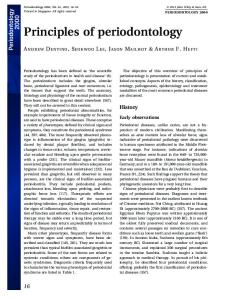
rates following a rise in atmosphericCO2 spanningcenturies, bit precisionof the calculation. doesthe effect of CaCO3 dissolutionbecomeapparent? In additionto time dependentruns,acceleration techniques The time courseof atmosphericpCO 2 specifiedby IPCC were usedto obtainvarioussteadystatesof the model (which scenario s750 [Schimel et al., 1994], offset by 33 gatm will be describedmore fully in Section5). A balancebetween (Figure l a) becausethe initial steadystateatmosphericpCO2 weathering andtheglobaldeepseaburialof CaCO3is referred of the model is higher than preanthropogenicby this amount
to as"globalsteadystate"andwasapproached by addingCO3= to the watercolumnhomogeneously, 10 timesper century,for
(see section 2). The allowed rate of terrestrial CO2 release was determined by holding the atmospheric CO2 at the 800 years. The CO3= concentration addedwas specified value and tabulating the flux of CO2 to the atmosphere/oceansystem which was required to track this CO3 =added = 50gmolL-• / GtC yr-•x [ weathering - burial ] specifiedconcentration.The resultsfor the no-CaCO3model The 800 yearacceleration periodwasfollowedby 700 yearsof are given in Figure lb; the resultswhich includedCaCO3 are spin-upto allowthe watercolumnchemistry to relaxtowarda nearly indistinguishableon this scale. The differencebetween the two is plotted as absoluteoceanuptakein Figure l c and as steady state. A separate steadystatecondition canbe called"localsteady a relative increasein Figure ld; this is the extra CO2 emission state,"definedas a balanceat eachgrid point betweenCaCO3 which is due to neutralization by seafloor CaCO3. The extra rain, dissolution,and burial. In local steadystatethe CaCO3 CO2 emission is at most a few percent, which is not lysoclineis stationarywith respectto a snapshotof water significantrelative to the uncertaintyof uptake by the ocean column chemistryand sedimentrain rates, but an oceanin or by the biosphere. We learn that the effect of deep sea
ARCHER ETAL.'FOSSILFUELCO2NEUTRALIZATION BYMARINECaCO 3
263
It appearsthat CO2 retentiontimes for the remaining atmosphere-boundfraction could exceed 500 years for marine disposal below a few kilometers [Hoffert et al., 1979]. Retention times can, however, be much shorter and have been
found to be dependenton the location of injection [Haugan and Drange, 1995]. Furthermore,there has been speculationthat
sediment dissolution can effectively increase the CO2 residencetime by preferentialdissolutionof CaCO3 in regions near or downstreamof the injection site. To assessthe effect of CaCO 3 dissolution on ocean disposal, we have run •
•
i--
3 2
emissions scenario A with 25% of theCO2 emissions injected
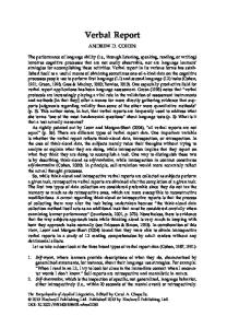
equally into the deep Pacific (east of Japanat 152.5ø E, 31.25ø N and 3000 m depth) and the Atlantic (Mediterranean outflow 0.08 water at 17.5ø W, 36.25 ø N and 3000 m depth). Figure 2 0.O7 shows that the effect of injecting 25% of the fossil fuel release 0.O6 0•05 directly into the oceansis much more significant than is the 0D4 effect of CO2 neutralizationby CaCO3. 0D3 0.O2 In addition, we have run more mechanisticallyinterpretable "impulse injection" experiments where 10 Gt C as CO2 is 0% impulse injected into the steady state ocean, comparing 3 Atlantic (17.5 ø W, 36.25ø N and 3000 m depth) vs. Pacific (152.5 ø E, 31.25ø N and 3000 m depth) both with and without CaCO 3. Figure 3 showsthe results of these experiments. Initially, the Atlantic injection modelstrack each other, as do 0,5 the Pacific, regardlessof the presenceof CaCO3, as we would o expect. The Pacific injection is somewhat "leakier" because 2(350 2100 2150 2200 2350 2300 Year the Pacific is closer to the end of the line of the deep sea circulation, which leads to a faster outgassing of the Figure 1. (a) Atmospheric pCO2 specified by the Intergovernmental Panel on ClimateChangefor a case(s750) atmospheric fraction of the CO2 impulse and also a slight where atmosphericCO2 approachesa stableconcentrationof overshoot on the approach toward atmosphere/ocean 750 ppm, offset by 33 gatm because of the higher than equilibrium. One thousandyears after the injection, the model observedmodel preanthropogenic pCO2. (b) Calculatednet runs sort themselves according to the presence or absenceof terrestrial emission of CO2 to match the s750 atmospheric CaCO 3. Dissolution fluxes (Figure 3b) are initially much concentrationfor both the CaCO3 and the no-CaCO3 models higher in the Atlantic injection experiment than in the Pacific (which are indistinguishablefrom each other in the graph). or atmospheric,and the accumulateddissolutionanomaly due The difference between the calculated emissions using the to the CO2 injection is greatest for the Atlantic injection, CaCO3 and no-CaCO3models,in gigatonsof C (c) and as a presumably because of the abundanceof CaCO3 in Atlantic percentof net terrestrialemission(d). The kink at A.D. 2250 sediments. Interestingly, the atmospheric release results in is the transition to a constant atmosphericCO2 specified by greater accumulateddissolutionanomaly after 1000 years than the s750 scenario. does the Pacific injection, because the pathway from the •
o
CaCO3 dissolution on the CO2 concentration over the next severalcenturiesis likely to be negligible,consistentwith previousstudies[Sundquist,1986;Maier-Reirner, 1993a'
[-
. Atmospheric Injection•=-• - No CaCO 3
Archer et al. , 1997]. 700
4. DeepOceanDisposalof COz A numberof geoengineering techniques havebeenproposed to control atmosphericgreenhousegas concentrations or to limit potentialimpacts [Panel on Policy Implicationsof Greenhouse Warming, 1992]. Marchetti [1977] proposed
capturing CO2 emissions frompowerplants anddisposing of
5o0
300 1750
2000
2250
2500
2750
3000
Year
it in the deepsea. Relativeto humanemissions, oceanshave
animmense capacity forCO2, sothattheadded burden of CO2 Figure 2. The calculated atmospheric responseto a direct
will be relativelysmall. Also,we will seein section5 thatthe oceandisposalof 25% of the net terrestrialemissionderrived ultimatefate of mostof the fossilfuel CO2 will be to dissolve from IPCC scenarioA to the year 2100, both with and without in the oceanseventuallyanyhow,so direct injectionwould CaCO3. CO2 is injecteddirectlyto two grid points,locatedat only be catalyzingthe transitionto an alreadyinevitable 3000 m depth in the Atlantic (17.5ø W, 36.25ø N) and Pacific condition.
(152.5 ø E, 31.25 ø N) oceans.
264
ARCHERET AL.' FOSSILFUELCO2NEUTRALIZATIONBY MARINECaCO3
5. Long Term Fate of Fossil Fuel CO2
1
0.8
(:• • • 0.6 0.4I f •
We havedonea seriesof time dependentmodelintegrations to characterize the millennialtimescalefate of fossilfuel CO2. These results have been briefly describedby Archer et al., [1997]; here we presenta morethoroughand detailedanalysis.
CaCO3
0.2
IPCC[Houghton et al., 1990,1992]hasputforthfamiliesOf
0
0.146
scenariosfor future emissionsof CO2 which have been used as benchmarksfor comparingcarbon cycle models [Enting et al., 1994] as well as making projectionsof global climate change and its impacts. Using simple ocean and biosphere carbon cycle models,IPCC projectedthe concentrationof CO2 in the atmospherein responseto these emissionsscenarios. Because we have no land biota model, our strategywas to imposethese projected CO 2 concentrations on the model atmosphere
1
Atmosphere
0.145 .•_
• • •
0.144 0.143
-•.;...;::: •
..--c:._::::.:::::....-.:.. .........
Atlantic
(.3
0.142 0.141
I
I
I
beginningat an initial steadystatein the year A.D. 1750. For <
-3
'F,o
m•
the period from 1750 to 1990, atmosphericCO2 was imposed at historicalvalues [Marland et al., 1993]. From 1990 through
-2
to A.D. 2100 we specify atmospheric concentrationsat
._
...m
-1
E
O
0
0
500
Pacific I I
c ½
1000
2000
1,500
projections based on the IPCC emissions scenarios labeled "Business-as-usual"and "B" [Houghton et al., 1990]. These projections include the effect of a terrestrial biospheric sink
for CO2. Following A.D. 2100 we chose several variants.
Yearsfromlnjection
The first two, which we label scenarios "A" and "B", follow the
Figure 3. Impulseinjectionexperimentresults,comparing the effectsof the locationof the injectionandthe presenceor IPCC 1990 scenariosBusiness-as-usualand B, respectively, absenceof CaCO3 in the model. Ten gigatonsof CO 2 is until A.D. 2100, and have zero emissions after A.D. 2100. injectedinto a steadystateocean(no risingatmospheric value) Scenarios A22 and A23 follow Business-as-usual until A.D. in the Atlantic or the Pacific oceans, both with and without
2100, then linearly extrapolate from the A.D.
CaCO3. andinto the atmosphere (whichis equivalent to a 4.96 gatm step-increasein atmosphericCO2 concentration)with CaCO3 dissolution.(a) Atmospheric pCO2 concentration, (b) CaCO3 burialrate, and (c) cumulativeburialanomalyrelative
terrestrial emission rate to A.D. 2200 or A.D. 2300, respectively, and thereafter the rate is set to zero. Following the emissionperiod, no further biosphericuptake was allowed; the system was closed except for weathering and sedimentation. The rate of net terrestrial emissionof CO2 is shown in Figure 4, and the cumulative emissionsof CO2 are
to the initial steady state.
summarized
atmosphere to the ocean is through the Atlantic, which the Pacific injection skips. However, the benefits of lowering the atmospheric CO2 transient by Pacific injection would appear to outweigh the drawbacksof leaking to the atmosphereand depressedCaCO3 dissolutionwhich Pacific injection appears
1.
Global
reserves
of fossil fuels have
been estimatedto be on the order of 5000 Gt C [Sundquist,
2000 1800 1600 1400
to generate. These
in Table
2100 net
results are consistent
with
earlier
studies.
Bacastow
1200
and Dewey [1996] speculatedthat CO2 injection at sites near the east coast of the United
States or in the North
would
calcite
benefit
more
from
dissolution
Atlantic
relative
200
to
0
injection in the Pacific. Using a four box model for atmosphere/ocean/sediment system, Cole et al. [1993, 1995] conclude that the extent of CaCO3 dissolution will vary significantly with injection depth. Nihous et al. [1994] found extensive
sediment
dissolution
when
a model
with
A23
fast
A22
dissolution kinetics was used. However, we find that the effect
of enhanced CaCO3 dissolutionin Atlantic CO2 injection (relative to atmosphericrelease) will only have an effect on pCO2 after roughly 500 years, and this effect will likely be compensatedby the enhancedproduction of CO2 [Kheshgi et al., 1994] required to carry out the capture and deep-sea injection of CO2. For thesereasons,we would not expectthe extent of enhanced CaCO3 dissolution to be an important factor in determiningthe effectivenessof deep sea disposalof CO2.
1000 0 1700
1800
1900
2000
2100
2200
2300
Year
Figure 4. (a) Time seriesof atmosphericCO2 concentration imposedon the model. ScenariosA, A22, and A23 stoptheir CO 2 releaseat the year 2100, 2200, and 2300 respectively. (b) Cumulative net terrestrial CO2 release for the four scenarios.
ARCHER ETAL.'FOSSIL FUELCO2NEUTRALIZATION BYMARINECaCO3 7
Table 1. Cumulative CO2 Emissionsfor Model Runs Driven by ExtendedIPCC Emission
265
7
Scenerios
Scenario
CO2 Release,Gt C
B A A22
874 1506 3028
A23
4550
B Mirror
-878
I
2
2000
2500
3000
2000
4000
6000
8000
10000
Year
Figure 6. (a) The e-foldingtime for invasionof CO2 into the oceanscan be estimatedfrom the slopeof the log of the model pC O2 (in microatmospheres) for the case of no CaCO3
1985],whichindicates thattheeventual release(beyond A.D. 2100)couldgreatlyexceedthecumulative releaseof theIPCC scenariosout to A.D.
•,3
0
2100. The models were run both with
dissolution(model - initial) versustime. The timescaleis 250-
400 years,longer for higher CO2 releasescenarios.(b) The timescale for the effect of CaCO3 on the pCO2 of the atmosphere can be estimatedfrom the slopeof the log of the
andwithoutCaCO3 compensation until A.D. 10,000,except difference between the model runs with and without CaCO3 versustime, ApCO2, defined as
for A22 which was extended to A.D. 40,000.
5.1.
z•9CO2 =(pCO2w,thCaCO 3--pCO2caCO3,final ) --(pCO2no CaCO3pro 2no CaCO3,tinal )
CO2 Invasion Timescale
Time seriesof atmospheric pCO2to A.D. 10,000are shown
in Figure5. The initial increasein atmospheric CO2 is
determinedby the emissionsscenario,and the subsequent This timescaleappearsto be about5000 yearsand relatively decline is caused by dissolution of CO2 in the oceans independent of theCO2 releasemagnitude. (invasion)and reaction with CaCO3 (neutralization). The characteristicsof invasion alone can best be determined from
the modelresultsneglectingCaCO3 dissolution(Figure 6a). Previous studiesof theoceanuptakeof a singleimpulseof CO2 release[Maier-Reimer and Hasselmann,1987; Sarmientoet al., 1992] resolved CO2 invasion into several distinct timescales corresponding to uptakeinto surface,thermocline, and intermediateand deep waters of the ocean. In our simulations, the hundredyear timescaleof the CO2 releasehas obscured the shorter timescales for ocean invasion. However,
we find thatthe overallCO2 declinecanbe approximated with singlee-foldingtimescales of 200 to 450 years,depending on
the amount of CO2 released (Table 2).
When CaCO3
dissolutionis disallowed in the model, the final equilibrium betweenthe oceanand the atmospherefinds 70%-81% of the
fossilfuel releasesequestered in the oceans(Table 2). These resultsare consistentwith Sundquist [1990b]. 5.2.
Reaction with CaCO3
The long-termeffectsof CaCO3 weatheringand seafloor dissolution on thepCO2 of the atmosphere canbe seenas the divergence betweenthesolidcurves(includingCaCO3)andthe dashed lines (no CaCO3) in Figure 5. In the initial millennium, there is little difference between the two model
2000
formulations, but beyondA.D. 3000, the reactionof CO2 with
CaCO3 _ noCaCO3
800
•
CaCO3 becomes significant.ThepH equilibrium chemistry of dissolvedCO2 leadsto an inverserelationship betweenCO2 and CO3=, whichcanbe seenas a decreasein deepPacific [CO3=] followingthe CO2 invasion(Figure7). This,in turn, provokestwo distinct but complementaryneutralization responses: dissolution of previouslydepositedCaCO3 on the
600
400
200 000
800 600
seafloor and net dissolution of terrestrial CaCO3 which is
400
temporarilynot balancedby seafloordepositionof CaCO3. This distinctionwill be justified in section5.5.
200 0
1000
2000
3000
4000
5000
6000
7000
8000
9000
10000
Year
By the end of the simulations, significantfractionsof the global inventoriesof CaCO3 in the bioturbatedlayer and within reach of chemical erosion have been exhausted.
The
initial e-folding time for the removal of CO2 by CaCO3, Figure 5. Model responseto anthropogenic CO2 releaseto relative to the caseof no CaCO3, is 5-6 kyr and relatively the year A.D. 10,000, includingthe effect of CaCO3 (solid of the magnitudeof CO2 release(Figure6b and curve),andneglecting CaCO3 (dashed curve).ThepCO2 is held independent Table 2), based on a plot of the log of the increasein the to IPCC projections for scenarios A andB to theyear2100and extrapolated to the years2200 and2300 at the scenario A year ApCO2 (CaCO3 - noCaCO3) towardthefinal steadystatevalue 2100 emissionrate for runs B, A, A22, and A23, respectively. givenin Table2. As we shallsee,thiscanbe takento be the After those times, a zero net terrestrial release of CO2 is specified.
timescaleof "seafloor"neutralizationeffect on the pCO 2 of the atmosphere.
266
ARCHERET AL.' FOSSILFUELCO2NEUTRALIZATION BY MARINECaCO3
Table 2. Summaryof OceanEffectsin the Model Analyses of the Extended IPCC Emission Scenarios
20,000 appearsto takeplacewith an e-foldingtimescaleof 18 kyr (Figure 9c).
B
A
A22
A23
Initial alkalinity
40510
40510
40510
40510
Gt C equivalents a Initial CO2 inventory
38400
38400
38400
38400
The divisionof CaCO3 compensation responseof the ocean into several componentshas been a commonfinding of previousstudies. Sundquist[1990a]partitionedthe alkalinity responseof the oceaninto primary and secondaryresponses basedon the log slopeof the modelresponse; theseresponses
Gt C
Initial erodibleCaCO3 Gt Cb InitialpCO2 Invasion•, yrc
1570
1570
1570
1570
310 212
310 255
310 365
310 453
Invasion finalpCO2 d
394
463
685
995
InvasionCO2 uptake e, %
80.7
79.6
75.1
69.7
Seafloor neut. •,fyr (
5480 5490 5870 6810
Seafloorneut.pCO2
355
390
497
Seafloorneut.CO2 uptakeg, % Seafloorneut.final alkalinitya
9.0 41611
9.8 42337
12.5 14.8 43831 44761
Seafloor neut. erodible CaCO 3b
1230 975
Terr. weat. •¾
Equilibrium hpCO 2 Equil. hCO2 uptake, % Equil. halkalinity 1 Equil. hCO2atm.residual e,%
424
661
a
•A23
129
8260
343 2.9 42015 7.5
366 3.2 43060 7.4
425 4.8 45588 7.6
489 7.6 48104 7.9
^23
aTheocean inventory of alkalinity, scaled to bedirectly comparable tocarbon inventories. Thescaling factor is 12g eq-1.
bExpressed in mass ofC, notCaCO3, fordirect comparison with
other carbon inventories.
2450
CDetermined by linearregression of ln[pCO2(t)-pCO2(final)] versus time for a time interval 2250 < t < 3000 A.D.
dFinal pCO 2ofthemodel neglecting CaCO 3.
02[
eExpressed aspercentage of thereleased CO2
fDetermined bylinear regression ofthelogofapproach tothefull effect of CaCO3 onpCO2, versustime as definedin the captionto
•
.0.1
Figure 6b. Regressionwas performedon model results2000 < t <
-02
10000. FinalpCO2 valuesfor the CaCO3 experiments aretakenfrom
.0.3
the equilibriumresults(see footnoteh).
gSameas footnotef but overtime interval10,000< t < 40,000. Model resultsfor the A22 scenarioonly.
--Weathering
0
ß 0.4 I •A23 C
(.3
hDetermined byacceleration of themodel to steady state where
.05
weathering is balanced by burialandthelysoclineis in localequilibrium with the water column saturation horizon.
None of the model results in Figure 5 have reestablished equilibriumby the endof their 10 kyr runs. This canbe seenin
Figure7c as the imbalancebetweenweatheringand deepsea CaCO3 accumulation andthe depletionof the seafloorCaCO3 inventory relative to the initial (steady state) condition. Figure 8 showsA22 to the year 40,000, by which time the global oceanburial rate and the seafloorCaCO3 inventories appearto have largely returnedto their original values. The efolding timescales for the approach to weathering / accumulationsteadystate ("terrestrial neutralization")can be estimatedfrom semilogplotsin Figure 9. In the first 10 kyr, both the atmosphericCO2 decline and the recovery of weathering/ burial steadystate relax to their final stateswith e-foldingtimescales of 5.5-6.8 kyr (Figure9a). After the year 10,000, the slope shallowsto an 8.3 kyr timescale. This is becausethe seafloorCaCO3inventoryhasreacheda minimum value and has been exhaustedas a sourceof alkalinity to neutralize CO2 (see section 5.5). The remainingsource, terrestrial CaCO3, is slower than seafloorneutralization. The replenishment of the seafloorCaCO3 inventoryafter the year
"-'
.o_
0
16130
U.I
0
2(XX)
4000
6000
8000
10000
Year
Figure 7. Model responseto the year A.D. 10,000 of (a) deep Pacific [CO3=]. (b) Alkalinity of the deep Pacific ocean. (c) Global accumulationrate of CaCO3 with negative values denoting net erosion. (d) Inventory of CaCO3 within the bioturbatedlayer on the seafloor. (e) Inventory of CaCO3 within the potential reach of chemical erosion on the seafloor.
ARCHER ETAL.:FOSSIL FUELCO2NEUTRALIZATION BYMARINECaCO3
267
1600
1400
= constant
which relates the partial pressureof CO2 exerted by a seawater sample and the concentrations of carbonate and bicarbonate ions to the apparent dissociation constantsfor carbonic acid
(K/' andK2') andthe Henry'slaw solubilityproductfor CO2 (KH). For the global ocean and atmosphere,the situation is complicated by heterogeneities in ocean chemistry and temperature,but we will retain the idea that the ratio on the left hand side will behave as a nearly constantvalue as the carbon inventories of the ocean and atmospherechange. Taking the ratio of initial and final states of the ocean/atmosphereand rearranging, we get the approximation
0.15 0.1
0.06
"IWealbering •
o >'-0.1 -0.15
-02 -03
pCO2ri.• = HCOjtin•CO•'initia 1 pCO2initialHCO•'initialCO3•m where the constantshave canceled and where we now replace
Erosionally •'••
ted••••'-•• B ionia •r
-O5
c
B
'õ
-2
0
Figure 8. Model resultsof (a) atmosphericpCO2, (b) CaCO3 accumulationrates, and (c) CaCO3 inventories for the A22 emission scenariointegratedto the year A.D. 40000.
o)
-25
•:
-3.5
--
2000
4000
6000
8000
10000
1Ok
20k
30k
40k
ranged from 1500 to 2700 and 10,800 to 14,200 years, respectively. The former was identified as seafloor neutralization,
because
it
was
sensitive
to
sediment
dissolutionkinetics,while the latter correspondsto the CaCO3 compensation (weathering / burial imbalance) timescales as estimated by Broecker and Peng [1987] and Boyle [1983]. Walker and Kasting [1992] assumedas an upper limit that seafloor dissolution occurs instantaneously, so that the several thousand year responsetime of their model to fossil fuel invasion represents only what we have called terrestrial neutralization.
5.3.
0
6.5
•A22
CaCO 3 Steady State
The final state of the 40 kyr A22 integration has nearly restoredthe seafloor CaCO3 inventory to original values, and the global burial rate balancesweathering. This state has also been obtained directly by the acceleration technique described in section2. The resultingalkalinity of the oceanand pCO2 of the atmosphereare given in Table 2. We find that even after complete reaction with CaCO3, approximately7-8% of the fossil fuel CO 2 remains in the atmosphere,consistent with Sundquist [1990a] and Walker and Kasting [1992]. The equilibrium partitioning of fossil fuel CO2 between the atmosphereand the CaCO3-bufferedocean can be understood from the aqueousCO2 equilibrium reactions. Dissolved CO2 equilibrium can be expressedas
c
1ok
20k
30k
40k
Year
Figure 9. (a) E-folding timescales of the return to a balance betweenweatheringand burial of CaCO3 for the A22 scenario. Slope of curves from A.D. 2000 to A.D. 10000 indicates timescales of 5480-6810 years (see Table 2). (b) Return to weathering/ burial steadystate over 40 kyr of model time, A22 scenario. The relaxation timescale slows to 8260 years after the year A.D. 10,000. (c) The timescale for restoration of the equilibrium depth of the lysocline is 18.1 kyr from the 40 kyr A22 model results, based on the log of the bioturbated layer CaCO 3 inventoryrelative to the initial value.
268
ARCHER ET AL.: FOSSIL FUEL CO2NEUTRALIZATION BY MARINE CaCO3
concentrations of bicarbonate and carbonate with global inventories, which we denote by dropping the brackets. Equilibrium with CaCO3 (the neutralizationreaction)tendsto
5.4.
Sensitivity to CaCO 3 Dissolution
Kinetics
Dissolutionof CaCO3 in the laboratoryhas been shownto exhibit a nonlinear dependenceon the undersaturationof the restoreCO3- to closeto its initial (equilibrium)value,reducing solution, attributed to dissolution as the sum of a range of the final factor on the right hand side to near 1. This leaves elementary reactions (CaCO 3 reacting byitselftoproduce Ca2+ atmosphericpCO2 to scalewith the bicarbonateinventoryof + CO3- or reactions coupledwith H+ or H2CO3)anda rangeof the ocean squared. We make a final approximationthat the typesof crystalsites(comer and defectsitesas opposedto flat relative increase in ocean bicarbonate should be about the same as the relative increase in total carbon in the ocean, since bicarbonate is the dominant form of carbon while the second
most important form, carbonateion, is held constant. This leaves us with the approximaterelation
pCO2nnai (•CO2o•ean +2XCO2ff )2 pCO2initial
2
ZCO2ocean
where the final total CO2 inventory of the ocean is approximatedas the initial value plus twice the fossil fuel CO2 release;the factor of 2 is due to the nearly 1:1 reactionof CO2 with CaCO3, which releasesadditional carbon to the ocean. For the A22 scenario, the initial total CO2 inventory is 38,400 Gt C, the fossil fuel release is 3028 Gt C, and the
predictedequilibriumpCO2 is 34% higher than the initial value (compared with 37% observed in the full model), accounting for 6.7% of the fossil fuel release (compared with 7.6% observedin the full model). We concludethat the residualCO2 left in the atmosphereafter complete reaction with CaCO3 is a straightforward result of equilibrium chemistry of inorganic carbon. This result is therefore likely to be relatively robust and model independent. The atmospheric residual will be buffered by the silicate rock cycle, which would tend toward equilibriumbetween CO2 consumptionassociatedwith weathering of basic components
surfacesites) [Berner and Morse, 1974]. A dissolutionorder n of 4.5 has been observedin the laboratoryby Keir [1980], and has been assumedby in situ dissolutionrate studies[Archer et al., 1989; Berelson et al., 1990; Cai, 1992], although the dissolution order is difficult to constrain using the range of
saturation conditions found in the deep sea [Hales et al., 1993]. Recently,Hales [1995] hasarguedthat first-orderrate kinetics(n=l) may be more appropriatefor in situ conditions. Hales finds that the range of rate constantvalues k inferred from his in situdataspansnearly3 ordersof magnitude,while the same data can be fit using n-1 with only 1 order of
magnitudevariation,usingk valuesbetween0.1 and 0.01% day-]. The effect of higherorderdissolutionkineticsis to increase the sensitivity of the dissolutionrate to the degree of undersaturation
as undersaturation
statepore water concentration profiles. In any case,we expect that the differences between the two formulations may become
pronounced duringthe extremeacidification of the oceanafter fossil fuel uptake. For the deepsea,undersaturation values 1.10-3
41000
O. 17•!at•l '10 '4
1.10-3
[Walker et al., 1981; Berner et al., 1983]. This mechanism is
representsan increasein the direct radiative forcing from CO2, relative to the preanthropogenic concentration of 280 ppm, that is as large as the CO2 direct radiative forcing change on the glacial termination (from 200 ppm).
extreme.
compensated for by changesin the diffusion/reaction steady
metamorphic decarbonation and volcanic degassingof CO2
3000 Gt fossil fuel release (scenario A22) will be an atmospheric pCO2 value of approximately 400 ppm. This
more
dissolutionrate constantare more difficult to predict, because the differences in the microscopic rate law may be
of silicate rocks such as CaO, and the reverse of this reaction,
thought to stabilize atmospheric CO2 on a time frame of several hundred thousandyears. The long time frame for this mechanism, relative to the glacial / interglacial cycles, raises the questionof what value for atmosphericCO2 is requiredto achieve balance between weathering and metamorphism. The question is complicated by fluctuations in both atmospheric CO2 and presumablyin silicate weatheringassociatedwith the climate cycles, but presumablythe true equilibriumCO2 value is somewherebetween the glacial and interglacial values. The 7-8% atmosphericresidualof the fossil fuel CO2 would, according to our current understanding, raise the baseline atmosphericCO2 concentrationfor a period of severalhundred thousandyears. This long tail on the fossil fuel CO2 forcing of climate may well be more significant to the future glacial/interglacial timescale evolution of Earth's climate than will the brief period of greater intensity warming, since its duration is greater than a glacial cycle. The end result of a
becomes
Within the diffusive pore water medium, the effects of the
3.10-4
39500
1.10-4
o
37500
3'10'5 o 37000
0
500
lOOO
15oo
2000
Bioturbated Lair CaCO3 Inventory Gt C
Figure 10. Steadymodel statesgeneratedin an effort to tune the model for linear dissolutionkinetics. Equilibrium model dependenceof alkalinity and CaCO3 inventorieson weathering
rate(equalto 0.145Gt C yr'] for opensymbols and0.175Gt C yr'l for solidcircles).Circlesarethelinearratelawmodelwith ratecoefficients rangingfrom3'10'5 to 1'10-3d'] asindicated. Diamonds are 4.5 order rate law (nonlinear) model with rate
coefficients of 1 and0.1 d-] asindicated.Thesquare is a databased estimate from the real ocean.
ARCHERETAL.' FOSSILFUELCO2NEUTRALIZATION BY MARINECaCO3 (expressedas ACO3 = [CO3-] - [CO3=]saturation) as low as -40
269
Year
•tmol kg'] are observed in the deepPacific,but calciteis
o
2(x)o
4000
6o(x)
8o(x)
1ocxx)
generally completelydepletedfrom these sediments;the range
of ACO3 across thelysocline is of order20-30•tmolkg'] in ACO3. Across this range in undersaturation,the difference between 1.0 and 4.5 order kinetic rate laws may be rather
-0.15
subtle. In contrast,deep sea [CO3-] suddenly decreases60
-0.2
•tmolkg'] followinga largefossilfuelCO2release(Figure7), in contact with sediments where CaCO3 has not yet been depleted. Under these conditions,the two kinetic rate laws may differ significantly in their neutralization and CaCO3 compensation responses. The comparison between linear and nonlinear CaCO3 dissolutionkinetics required first spinningup the model to a steady state using linear dissolutionkinetics in the sediments. We found that simply changingthe dissolutionorder and rate constant to linear kinetics consistently underrepresentedthe inventory of CaCO3 in surfacesediments(Figure 10). This becomes significant as CaCO3 is depleted from surface sediments;the lower inventory decreasesthe dissolutionflux, obscuring the differences between the two kinetics formulations. Linear kinetics generate a lower CaCO3 inventory when everythingelse is equal becausethe lysocline tends to be sharper using linear kinetics. For a given weathering rate (which determinesthe area of high-CaCO3 sedimentswhere most of the CaCO3 burial occurs), there is a smaller area of moderate-CaCO3 concentrationsedimentsto contribute to the CaCO3 inventory using linear kinetics; CaCO3 concentrationtends to be more focusedinto areas of high accumulation. Varying the dissolutionrate constantk had the effect in the steady state of changing the saturation state of the whole ocean (representedin Figure 10 by the alkalinity inventory), without much of a change in the bioturbatedlayer CaCO3 inventory,which is determinedby the global burial rate. In other words,the rate constantaffectsthe ACO 3 of the lysoclinewithout changingthe thicknessof the transition zone very much. We found that to reproduceboth the alkalinity and the CaCO3 inventories of the nonlinear model, we were forced to increase the weathering rate from
-0.25
•
Nonlin
I
Linear
I..................... NonlirtSlow
9OO
ß
800 700
600
$oo
4oo
L _
LineaSlo
300
200 100 0
o
2000
4000
6000
8000
10000
Year
Figure 11. (a)CaCO 3 burial anomaly (deviation from steady state value) and (b) atmosphericpCO2, a comparisonbetween linear (first order) versus nonlinear (4.5 order), and fast versus slow
dissolution
kinetics.
Rate
constants
are
as follows:
nonlinear,1.0 day']' nonlinear slow,0.1 day-]' linear,1'10'3 d']' linearslow,1'10'4 day']. Weathering ratesare0.145Gt C yr'] for nonlinearmodelsand 0.175 Gt C yr-] for linear models.
formulationof the kineticrate law hassurprisingly little effect on the neutralization of fossil fuel CO2, except for the magnitudeof the dissolutionspike immediatelyfollowing invasionfor the slow linear model,and interestingly,only the linear model is sensitive even in this time period. The dynamicsof the dissolutionspikeare exploredbelow. 5.5.
Analysis
and
Discussion
5.5.1. A Phase Diagram for CaCO3 Compensation. AnthropogenicCO2 can be viewed as a perturbation
0.145Gt C yr'] to 0.175Gt C yr-], thusincreasing the global of two natural cycles of carbon on the surface of the earth: CaCO 3 compensation in the ocean and the silicate rock weathering/ volcanic degassingbalance [Walker et al., 1981; Berneret al., 1983]. The interactionof the CO2 perturbation kinetics. with thesenatural cyclesis controlledby the dynamicsof the A comparison of the global burial rate of CaCO3 is system,which we undertaketo analyzehere. Thesedynamics of carboncycle presentedas deviationsfrom the initial steady state value in will alsoeventuallyapplyto our understanding Figure11. We seethatforn=l andk=l0'3 day'] (thefastlinear rearrangements corresponding to the glacial interglacial model) the results are indistinguishablefrom the results using transitions. The response of the model to fossil fuel invasion is a n=4.5andk=l day'] (thenonlinear model). Thisis alsotrue for the slow nonlinearmodel (n=4.5 and k=0.1 day']). relaxationtoward a new steadystatecondition. An analogy burial rate of CaCO3. However, the global burial rate is not known to this precision, so that the contrast in burial rates cannotbe construedas an argumenteither for or againstlinear
However,whenn=l andk=10'4 day-] (theslowlinearmodel)
can be drawn to the dissolution of a solid material in a beaker
the initial spike in dissolutionintensity is attenuated,but the long-termtrend in dissolutionconvergeson the time trend of the other models. The CO2 historiesof the three models are shown in Figure l lb, and again we find relatively minor differences. The slow nonlinear model lags in the uptake of fossil fuel CO2 by about 10 ppm throughout the simulation, while the pCO2 of the fast linear model is consistentlyabout5 ppm lower than the nonlinear model (largely an offset due to the difference in steady state initial conditions). The
in the lab. The kineticsof this systemare describedby rate equations, which will require at least two pieces of information, the extent of disequilibrium (in this case a propertyof the solution)and the quantityof the solid phase reactant (or more precisely the surface area).
We will
characterizethe dynamicsof the ocean/sedimentmodel by ignoring spatial heterogeneityand reducing the complex three-dimensionalcalcite saturation state (defined by the deviationof CO3= from saturation, ACO3) and%CaCO3 fields
270
ARCHERET AL.' FOSSILFUEL CO2NEUTRALIZATIONBY MARINE CaCOs
0.5
0.5 B Mio
•--
•
•
•
•
0.5•
g
[!,!111
?_,,3
I
I vsocline
0'5
i I I ! i i.i,
c_.
T-/
!
o
Influx
Influx
Influx
Throughput
EndofSeafloor
B
Neutralization
,....
0
B
A A22
-0.2
A23
-0.53O 1600 9O
800
-0.5
400
120
•O qe•&O•
1600 30
400800• Inje• • ion•Global Throughput 9O
quilibrium
120
• Sea Floor
•'
Diss
Local Lysoctine Equilibrium 1600 B dirro
' 60
/
1200 '
End of Sea Floor ••., eathering Neutralization 90 Neut. 400
YearA.D.
400o moo re(x) •o, eoo
800
120 0
Plate 2. The two variables which largely determine the global accumulationrate of CaCO3, deep ocean [CO3=] and the bioturbatedlayer CaCO3 inventory,are plotted againstthe model CaCO3 burial rate response. Spheres and the red line representsynchronybetween the calcite lysocline and the water column saturation state (the steadylysocline regime). Cubes and the green line representthe state of weathering! burial steady state for CaCO3 (the steady throughputregime). Time dependentresponseto CO2 invasion is shown as multicoloredlines, with model time indicatedby the color scale, which resetsto zero every 10 kyr for the 40 kyr A22 scenariorun. Initial invasionof CO2 depletesdeepocean[CO3=], which is subsequently replenished as mixed layer CaCO3 is depleted. Once the model trajectbry intersects the steady lysocline line, neutralization of CO2 by chemical erosion ceases. Symmetry of the model responseis shown by removing CO2 from the atmospherein a mirror image to scenarioB, which tracesa complementarypath to B. to single values. These values will be the concentration of These two state variables for the ocean carbonate system CO3= from a singlearbitrarylocationin the westernequatorial correspond to reservoirs for carbonate with fluxes between Pacific (170øW, 1.25øS and 2000 m) representing the them. The reservoirsare the [CO3=] of the ocean,determined saturation state, and the global inventory of CaCO3 in the by the alkalinity and ZCO2, and the inventory of seafloor sediment bioturbated layer,representing thesurface areaof CaCO3 available for dissolution(Figure 12). The input to the substrate. By reducing the state of the ocean to these two system is weathering, which transfers alkalinity to the ocean. variables, we are assumingthat the ocean state associatedwith Output consists of the imbalance between the rain rate of a given value of one of these variables is single valued, in CaCO3 to the seafloorand the seafloordissolutionflux, which other words that a single pair of numbersis all that is required we will call the "accumulation" rate of CaCO3 (the middlearrow to describethe carbon cycle in the ocean. Of course, the state in Figure 12). Finally, CaCO3 is effectively removedfrom the of the ocean cannot be exactly represented by these two system as it escapes the potential reach of seafloor The final removal of sediment from the ocean variablesalone. However as we will show, this approximation dissolution. simplifies our interpretationof the behavior of the model as a system will be called "burial," the bottom arrow in Figure 12. dynamical system. Also, we shall see that the limitations of Because the burial rate is defined relative to the deepest this approachare themselvesrevealing of the dynamicsof the possible reach of chemical erosion, its value can never be model. negative, since by definition CaCO3 below the erodible depth
ARCHER ETAL.'FOSSIL FUELCO2NEUTRALIZATION BYMARINECaCO3
Terrestrial 1
Weathering
Ocean
271
The steadystateconditionfor the erodibleCaCO3 inventory (equation 2) is the condition of local balance in the budget for CaCO 3 in the sedimentmixed layer, where at each model grid point
Alkalinity
CaCO3 rain- dissolution + burial
StateVariable= [C• =]
For any distributionof [CO3-], there is a concentrationfield of CaCO3 on the seafloorwhich satisfiesthis condition. Because the equilibrium condition can be calculated locally, this steady state condition will hereafter be called local lysocline equilibrium. The set of local lysocline equilibrium states can be describedby a line on a deep Pacific [CO3-] / bioturbated layer CaCO3 phaseplot (Figure 13a). This line was calculated by (1) adjusting the [CO3-] of the deep sea by imposing a homogeneousoffset to the total CO2 of the water column,then (2) calculating the steady state concentrationof CaCO3 by
CaCO3 1
Accumulation
(net predpitation)
Erodible
CaCO3 State Variable =
Bioturbated CaCO• Inventory
CaCO3 1 Burial
(remo•l from erodiblela•er)
Figure 12. Fossilfuel neutralizationcan be conceptualized as a perturbationto the system of weathering, CaCO3 accumulation (defined as the instantaneousdifference between
CaCO3 depositionand dissolution),and burial (definedas the permanent removal of CaCO3 from the potential reach of chemicalerosion,or the flux of CaCO3pastthe erodibleline
can never be redissolved.
[003fi
Decreashg
in the sediments,defined in text).
Increashg
/• Increasng
The rate of burial as defined here is
• •.•creashg
determinedby the accumulation rate of non-CaCO3materialon the seafloormultipliedby the concentration of CaCO3 at the erodible depth. 5.5.2. Stages
d
of
the
Neutralization
Process.
The differentialequationdescribing ocean[CO3=] is
O[CO• ]=ax[weatheringaccumulation]-/5 xCO 2invasion Ot
(1)
A22 A•rror
[
wheret• and13representbufferingof ocean[CO3=] by the reactionwith dissolvedCO2. Thesecoefficientsare nonlinear functionsof the concentrations of CO3=, HCO3-, andCO2 but are always positive, so that an excessof weatheringover
accumulation alwaysdrivesan increasein ocean[CO3=],CO2 invasion always decreasesocean [CO3=], and a balance betweenweatheringandaccumulation, in the absenceof CO2 invasion,is the steadystate. Beyond this, the complexity intrinsicto t• and13neednot concernus here. The equationfor the bioturbated layer CaCO3 inventoryis
NorthPacific[003=•
pmol L'1
Figure 13. (a) Steadystateconcentration of CaCO3 at each grid point on the seafloor as a function of [CO3=] at an arbitrary location in the Pacific Ocean (170øW, 1.25øS and
2000 m). Above this "steadylysocline"line, the CaCO3 decreases with time, and below this it increases. Vertical axis
is the global inventoryof CaCO3 in the bioturbatedlayer. (b) Deep Pacific [CO3=] at whichthe oceanCaCO3 accumulation rate balancesthe terrestrialweatheringrate, as a function of the CaCO3 inventoryresultsof Figure 13a. To the left of the "steadythroughput" line ocean[CO3=] increases, to the rightit 8t decreases. (c) Time dependentbehavior of both variables, [CO3=] andCaCO3, from Figures13aand 13btendsto drivethe where accumulation is defined as the net sedimentation rate, model statetoward one of the regionsB or D. The full model which can be negativeindicatingchemicalerosion,and burial is the rate at which CaCO3 crossesthe erodible depth and steady state is given by the intersection of the steady lysoclineand the steadythroughputlines. (d) Model behavior becomesunavailablefor chemical erosion, a flux which by for the IPCC B, A, A22, and A23 scenarios(see Table 1). definition can never be negative. We leave a detailed Circles mark millennia. Simulationsstartedin steadystate, characterizationof thesefluxes, in particularthe accumulation and all went to 10 kyr exceptfor the A22 scenario,which went flux, to section5.5.3 but for the time being it is instructiveto to 40 kyr, long enoughto return to show the behavior of the derive numerically the steady state conditions for these two returntoward steadystate. The "B Mirror" scenariois merely variables,where the input and output fluxes balance and the the oppositeof the "B" scenario,with a CO2 drawdownflux time derivativesequal zero. that mirrorsthe CO2 releaseflux of the B scenario.
ø3erødible CaCO3 - accumulationburial (2)
272
ARCHERET AL.' FOSSILFUEL CO2NEUTRALIZATIONBY MARINE CaCO3 5000
Total:BmeckerandTakahashi,1978
4500 4000 3500 3000 2500
2000
Total:Amher, 1996 A22
1500
A23
ADissolved• A
1000
B
500 0
1000 1.0
2000
3000
4000
5000
Tota• seaflOOrcaCO3 I
0.8
•.
I
0.6
B A
: 0.4
A22• A23
0.2
b 1000
2000
3000
4000
5000
Gt C Released
Figure 14.
(a) Inventoryof dissolvableCaCO3 on the
seafloor. Dashed lines represent estimates of the total available inventories of CaCO3. Circles are amountsof
seafloorCaCO3 dissolvedas a functionof fossilfuel CO2 release.(b) The fractionof neutralization of the modelby the year 10,000 (circles), determined as the increase in model alkalinity relative to the difference between the initial and the
fully neutralizedstate(calculatedas explainedin text; results in Table 2). The increasein oceanalkalinityin the year 10,000 (squares)whichcorresponds to the decreasein erodible layer CaCO3 inventory relative to the initial condition. The boldline wouldbe theresultof dissolving theentire1800Gt C erodible inventory of CaCO3 on the seafloor (maximum neutralization). Figure 14 shows that (1) seafloor neutralizationaccountsfor most of the ocean alkalinity increasebeforeyear 10,000,but (2) seafloorCaCO3 is unable to neutralizethe entirenet terrestrialCO2 release,even when the CO2 releaseis smallerthan the "potentiallyerodible" CaCO3 inventory. The reasonfor thislimitationis explained in the text and in Figure 13.
iteration[Archer, 1990] as the modelchemistryspunup over 1000years. The resultinginventoryof CaCO3 wastalliedand plottedagainstthe corresponding valueof deepPacific[CO3=], to make up the steadylysoclineline in Figure 13a. Below the steadylysoclineline, the inventoryof CaCO3 is smallerthan the steadystatevalue,implyingthat• erodibleCaCO3 / •t > 0. Above, the erodibleCaCO3is declining. The global steady state of the model balancesinput of [CO3=] to the ocean from continentalweatheringagainst removalby CaCO3accumulation on the seafloor(equation1). This conditionwas alsofoundby acceleration.For eachof the steady lysocline experiments described above, after the distributionof CaCO3 was calculatedat somevalue of deep Pacific [CO3=], the concentrationof [CO3=] was increased iteratively over a relaxation time of 1000 years, until the global accumulationrate balanced the weathering rate. In contrastto local lysocline equilibrium, the weatheringequal
accumulation steady state is a global condition, and for this reasonthis statewill be referredto as global throughputsteady state. For any value of the CaCO3 inventory there is a corresponding value of ocean [CO3=] at which global throughputsteady state will obtain, so that global throughput steadystate also describesa line on the deep Pacific [CO3=] / bioturbatedlayer CaCO3 phaseplot (Figure 13b). The trendof this line is toward increasing deep Pacific [CO3=] with increasing bioturbated CaCO3 inventory (a positive slope). This is a somewhat counterintuitiveresult; one might have expected that more CaCO3 on the seafloor would tend to increase CaCO3 accumulation,requiring a lower [CO3=] to compensate. The observed behavior of the model can be understoodas follows. The steadystate requiresthat input from weathering, which is held constantin the model, balance the rain of CaCO3 to the seafloor,which is also held constant, minus seafloor CaCO3 dissolution,which is predictedby the model. Throughputbalanceis thereforedeterminedentirelyby
the dissolutionflux, which increaseswith increasingCaCO3 inventoryon the seafloor. As the CaCO3 inventory increases, a highervalue of [CO3=] (lesserundersaturation) is requiredto maintainthe requisitedissolutionflux. The steadythroughput line exhibits positive slope as does the steadylysoclineline, but a muchsteeperslope. The steadythroughputline describes the state 3[CO3=]/3t = 0; area to the left of the line has a positivegrowth,and area to the right has negativegrowth.
The division of the phase plane (Figure 13c) into four quadrants determines the behaviorof the dynamicalsystem shownin Figure 12. The signsof 3/3t for both statevariables
of the systemare indicatedin Figure 13. In region"A," the sediment inventorytendsto decrease whilethe ocean[CO3=] tendsto increase. The oppositesituationis foundin region "C." In this region, a transferof carbonbetweenthe sediment
and the ocean will act to satisfy the requirementsof both reservoirs;
the
evolution
of
"complementary" to each other.
both
reservoirs
are
In the case of excess
dissolution (regionA), we havealreadynamedthisresponse seafloor neutralization. The response time of seafloor neutralizationis relatively fast becausethe accumulationrate, the middlearrowin Figure 12, is limited only by the kinetics of CaCO3 diagenesis.The weatheringrate is held fixed and constant,and burial, the flux of CaCO3 acrossthe erodible line, is by definition nonnegative. In contrast, the accumulation rate flux is free to exceedweatheringor to reach negative values. Seafloor neutralization can be envisioned as
an internal transfer of CO3= within the ocean / sediment system,unboundedby the weatheringand burial fluxes. In the "uncomplementary"regions of the phase space, regions "B" and "D," both the ocean and the sediment evolve in the same direction; in the case of fossil fuel neutralization,
both await replenishmentby the excessof weatheringover burial (terrestrialneutralization). In this regime,the steady accumulation flux can be no greaterthanthe weatheringinflux nor smaller than the burial flux (which is limited to nonnegative values). The accumulation flux is therefore less dynamic in this case than it was when the model was in one of
the complementaryregions of the phase plot (A or C). Seafloor CaCO3 no longer contributesto the neutralizationof fossil fuel CO2. For this reason, model evolution in this regime is slower than in the complementaryregimes. The
ARCHER ETAL.'FOSSILFUELCO2NEUTRALIZATION BY MARINECaCO3 transition of the model into the uncomplementaryregime at
Table 3. Results of the Dissolution Flux Parameterization
aroundthe year 10,000 is the reasonfor the increasein e- Experiments foldingtimescalefor CaCO3burialafterthistimein Figure9b. By 10,000, the alkalinityof the oceanhas increasedto 60- DeepPacific[CO3=], 75% of its final (fully neutralized)value (Figure 14). Most of gmolL-1 this increasecorresponds to the decreasein erodibleCaCO3 inventory on the seafloor, leaving only a small role for 86.4 terrestrialCaCO3 throughthis time.
quadrants in phasespacetendsto drivethe modeltowardthe uncomplementary regions,whichserveas dynamicalattractors for the modelstate(Figure 13c). This is demonstrated by the modeltrajectories in Figure13d. Oncethe modelreachesone of theuncomplementary regions,it slowlyevolvesbackto the modelstartingpoint (the full steadystatecondition).As it doesso, it veersto the left, towardthe steadythroughput line,
indicatingthat the modelachievessteadythroughput (nearly steadyocean[CO3=])whilethelysoclinelagsbehind.
80
60
._o
a.
40
o
30
Z 20
0
200
400
600
800
1000
Bioturbated Layer
GlobalCaCO3
Gt C
1
CaCO 3 Inventory, Burial Rate, GtCyr-
79.1 72.0 65.2 58.8 52.6 47.0 87.0 78.4 70.2 60.3 52.7 45.8 39.5 85.3 76.5 67.1 58.5 50.2 42.9 36.3 85.0 75.7 66.1 58.8 50.1 42.3 35.6
The directions of model evolution in the complementary
C)
273
1200
1298 1244 1187 1130 1072 1015 958 834 763 699 662 613 565 522 440 382 330 318 284 252 225 245 185 135 139 117 102 90
0.113 0.031 -0.053 -0.135 -0.215 -0.289 -0.359 0.144 0.073 0.000 -0.053 -0.109 -0.161 -0.205 O. 170 0.099 0.049 0.011 -0.028 -0.061 -0.087 0.178 0.117 0.068 0.043 0.017 0.000 -0.015
Ocean [CO3=] and seafloorCaCO3 inventorieswere perturbed independentlyof eachother. The steadymodel CaCO3 accumulation rate is taken to be the flux 1100 years after the perturbation as a functionof the [CO3=] andCaCO3 valuesat thattime.
The relationshipof modelbehaviorwith the two equilibrium ._
o
0
200
400
200
400
600
800
1000
1200
600
800
1000
1200
0.3 02 0.1
õ
-.•
o
• •-•
-0.1
'•
-02
EO
>'
o •
-03
•.6
•.8
0
Years
Figure 15. The results of adding ]00 g M CO2, homogeneously, to the water column of the model, in year 100 of the simulation: (a) time trace of deep Pacific [CO3=], (b) bioturbated CaCO3 inventory, and (c) model CaCO3 accumulation rate. The accumulation rate "spikes" immediately following the acidification and decreases thereafter to a steady value. It appears that the decreasing dissolution flux over the next 1000 years is not simply a product of changesin deep Pacific [CO3=] (Figure 15a) or bioturbatedlayer CaCO3 (Figure 15b).
conditions is summarized in Plate 2, which relates the global accumulation rate of CaCO 3 to deep ocean [CO3=] and bioturbatedlayer CaCO3 inventory in three dimensionalspace and in three two-dimensional projections. The global throughputequilibrium condition (green cubes) can be seen to satisfy the constraint that accumulation equals weathering, while the local lysocline equilibrium (red spheres) does not satisfy this condition except where it intersects the global throughput equilibrium line. The model trajectories intersect the equilibrium conditions in three-dimensional space, supporting our contention that the equilibrium conditions (which were determined independently of the model trajectories) are relevant to the evolution of the model state. Finally, symmetry of the model evolution is demonstratedby a mirror image B scenario which removed CO2 rather than releasing it, which traces a complementarypath to B. 5.5.3. Control of the CaCO 3 Accumulation Rate.
We
have
seen that
the
behavior
of
the
model
is
determinedby the rates of addition and removal of CO3 from the ocean and surface sedimentaryreservoirs and the response of those rates to the fossil fuel perturbation. In particular, the accumulationflux of CaCO3 on the seafloordominatesthe fast seafloorneutralizationresponsein the 5 kyr or so of the model
274
ARCHERET AL.:FOSSILFUELCO2NEUTRALIZATION BY MARINECaCO3
runs. Previous estimates of the CaCO 3 compensation timescale [Boyle, 1983; Broecker and Peng, 1987; Sundquist, 1990a; Walker and Kasting, 1992] differed in part becauseof differencesin the presumedsensitivity of the global CaCO3 accumulation
rate to ocean
acidification.
In this section
we
characterizethe global CaCO3= accumulationrate of the model as a function of ACO3 and the bioturbatedCaCO3 inventory (1) for use in understandingthe model resultsand (2) for use in simpler parameterized models of CaCO3 compensation. Because we are parameterizing the dissolution flux as a functionof deepPacific [CO3=] and bioturbatedlayer CaCO3, we refer to theseas the parametricmodel experiments. The CaCO3 distributionon the seafloorought to resemblea natural model state, so we adjustedthe bioturbatedCaCO3 inventory of the model by adjustingthe water column [CO3=] (a homogeneousperturbation of water column total CO2), spinning up, and then calculating the steady state CaCO3 distribution. Following this, we again perturbed the water column [CO3=]. A sample result from one of these model experiments (the standard distribution of CaCO3 and a homogeneousaddition of 100 gM CO2) is shownin Figure 15. During spin-up, [CO3 =] increases somewhat and the bioturbated layer CaCO3 inventory decreases,as the model begins to neutralize the added CO2. Dissolution intensity reaches an intense maximum (a minimum in CaCO3 burial) directly after the CO2 addition and stabilizes at lower values after 1000 years. At this time the model is out of steadystate (by design), but the accumulationrate is relatively stable with respectto the currentvaluesof ACO3 and CaCO3. Summarizing results of many such model runs, the steady (1000 year) CaCO3 accumulation rates in Table 3 were empirically fit to yield the equation
Accumulation = 3.12542x10 -3GtC yr-] (gmolkg-])-1x [CO3 =] - 8.25096x10 -4Gt C yr-1(GtC)-•xCaCO 3 + 9.06625x10 -6Gt C yr-• (Gt C gmolkg-•)-lx [CO3=] x CaCO3
- 8.626211x10 -2Gt C yr-• Deep Padtic[CO3=]
90
pM 6(
30 0.5
-0.5
200
6OO
400
80O
Bioturbated CaCO 3 Inmntory Gt C
Figure 16. Comparisonof the steady dissolutionflux results from experiments such as shown in Figure 10, with a parameterized empirical function for dissolution as a function of deepPacific [CO3=] and bioturbatedlayer CaCO3 inventory.
0.15
0.1 I Param •
....
0
•>, (.•
• •
-0.05 -o,1
-0.15 -0.2
-0.25 -0,3 -0,35
o
10000
20000
30000
40000
o. 15
Figure 17. (a) A comparison of the full time dependent model results(A22) againstpredictionsof the dissolutionflux as a function of the time-evolving values of deep Pacific
[CO3 =] and bioturbated layer CaCO3 inventory. The parameterized function describes the time evolution of the model well, exceptthat it underestimates the magnitudeof the time dependent model dissolution flux in the millennium following CO2 release. (b) Detail of the first 5000 yearsof the experimentwith the same comparisonas (a) but also showing the dissolution spike, defined as the difference between the time dependentmodel results and the parameterizedfunction values. The timescale for decay of the dissolution spike resembles the behavior of the model in response to a homogeneousperturbation(Figure 10).
with a fit to the individual model resultsshownin Figure 16. The accumulationfluxes expectedfrom the model evolution of ACO3 and bioturbatedCaCO3 inventoryare comparedwith the actual model values in Figure 17. It can be seen that the empirically predicted accumulation rate corresponds well except for a significant spike in dissolution immediately following the fossil fuel invasion. Similar behavior was observedin the parametric model runs, a simple example of which was shown in Figure 16. The magnitude of the transitional dissolution spike was calculated by subtracting the model accumulation rate from the empirical prediction, in Figure 17(b). Both the magnitude and the decay time of the transient dissolution spike correspondwell to the initial spike of dissolutionfrom the model run in Figure 15. This observation motivates a closer inspection of the transient behavior of the parametric model run in Figure 15. Over 1000 years following the homogeneousaddition of CO2, the dissolutionflux decreasedmore than can be explained by the changing values of A CO3 = or bioturbated CaCO 3 inventory. This behavior was causedby a rearrangementof the distribution of ACO3 = in the water column, by a process analogousto the formation of a whole ocean boundary layer, causedby surface/ deep fractionationof alkalinity in the ocean analogousto the biological pump. The global productionrate
of CaCO3in themodelis approximately 1.6Gt C yr-•. Most of this CaCO 3 redissolves in the water column or at the
ARCHER ETAL.'FOSSILFUELCO2NEUTRALIZATION BY MARINECaCOs •co3 =
of 200-450 yearsdependingon the magnitudeof the fossil fuel release. (2) A fast seafloor dissolution spike after CO2 dissolvesin the oceansbut before alkalinity has a chance to
gM -lOO
-50
0
275
50
o-
reorganize accounts for half of the neutralization in the coming millennium and 10% of the total CaCO3 dissolutionin
responseto fossil fuel CO2. Beginningin this stage,mankind will have reversed the sedimentation rate of the ocean by dissolving CaCO3 faster than it is depositedon the seafloor; this is projectedto peak by the year A.D. 3000 and last up to 5000 years. (3) Steady seafloordissolutioncontinuesuntil the lysocline reaches local equilibrium with the water column saturation state by about the year A.D. 10,000. Seafloor
E
Initial 500
neutralization
years
Figure 18. A comparisonof profiles of ACO3= immediately followingand 500 yearsafter a homogeneous additionof CO2 to the water column, from 120øE, 0øN.
seafloor, concentrating alkalinity in the deep waters. The
dissolution flux from the sediments reached0.5 Gt C yr'], which acts as an added sourceof alkalinity to the deep waters comparable to the flux attributable to the biological pump. Over the courseof the 1000 year circulationtime of the ocean, the alkalinity of deep waters increaseduntil a balancebetween dissolution and deep ocean circulation was reached. This relaxation is analogous to the formation of a whole ocean boundary layer. Profiles of ocean alkalinity during the dissolutionspike and 500 years later are shown in Figure 18. The largest [CO3=] changesare found immediately above high %CaCO 3 areason the seafloor. In the IPCC model runs, the transient dissolution spike is responsible for 50% of the dissolutionflux to year 3000 and roughly 10% of the flux to the year 40,000. This transientdissolutionspike is the only case where the approximation of the ocean carbonatesystem as representableby two simple variables,deep Pacific [CO3=] and bioturbatedlayer CaCO3 inventory,breaksdown.
overall
accounts
for 60-70%
of the fossil
fuel
CO 2, and hasan e-folding timescaleof 5-6 kyr. (4) Terrestrial weatheringreplenishesocean [CO3=] on a timescaleof 8 kyr after A.D. 10,000 and restoresthe lysocline to its original depth on a timescale of 18 kyr. Completion of this stage leaves 7-8% of the fossil fuel CO 2 remaining in the atmosphere in a new local and global CaCO3 steady state. (5) Neutralization by the silicate rock cycle (not included in the model) restoresatmosphericCO2 to some unknown "set point", at which metamorphicdecarbonationbalances silicate weathering, with a time constant of several hundred thousand years.
Acknowledgments. This paper benefittedby reviews by Eric Sundquist,Scott Doney, and anotheranonymousreviewer, and was supportedby the Petroleum ResearchFund and the David and Lucille Packard Foundation.
References
Archer,D. E., The dissolutionof calcitein deepseasediments: An in situmicroelectrode study,Ph.D. thesis,Univ. Wash.,Seattle,1990. Archer,D., Modelingthecalcitelysocline,J. Geophys. Res.,96, 17,03717,050, 1991. Archer, D., An atlas of the distribution of calcium carbonate in
sediments of the deepsea,Global Biogeochem.Cycles,10, 159-174, 1996a.
Archer,D., A data-drivenmodelof the globalcalcitelysocline,Global Biogeochern.Cycles,10, 511-526, 1996b.
Archer,D., S. Emerson, andC. Reimers,Dissolution of calcitein deepsea sediments:pH and 0 2 microelectroderesults, Geochim.
6. Summary
Cosmochim.Acta, 53, 2831-2846, 1989.
Accordingto our currentunderstanding, CO2 uptakeby rock cyclesof the Earth will be slow, with no significantimpact on the pCO 2 of the atmospherefor the next thousandyears. The net
terrestrial
emission
calculated
to
meet
an
IPCC
atmospheric stabilization scenario (s750) is only a few percent higher when CaCO 3 is included in the model simulation,which is negligible comparedwith uncertaintiesin biosphericuptake or other aspectsof the ocean carbon cycle. Direct ocean injection experiments demonstrate a coupling between dissolution and ocean circulation, as CaCO 3 dissolutionproceedssomewhatmore rapidly for atmospheric and Atlantic injection cases than for Pacific injection. However, CaCO3 dissolutionwill play only a minor role in determining the fate of fossil fuel CO2 in the coming millennium.
On longer timescales,neutralization of fossil fuel CO2 by the oceans and by CaCO3 takes place in five stages. (1) Invasion of fossil fuel into the oceans will sequester7080% of the net terrestrialCO2 releaseon an e-folding timescale
Archer,D., H. Kheshgi,and E. Maier-Reimer,Multiple timescalesfor neutralizationof fossilfuel CO2, Geophys.Res. Lett., 24, 405-408, 1997.
Bacastow, R. B., andR. K. Dewey,Effectiveness of CO2 sequestration in the post-industrial ocean,Energy Conversi.and Manage.,37, 1079-1086, 1996.
Berelson, W. M., D. E. Hammond, and G. A. Cutter, In situ measurements of calciumcarbonatedissolutionrates in deep sea sediments,Geochim.Cosmochim. Acta, 54, 3013-3020, 1990.
Berner,E. K., andR. A. Berner,TheGlobalWaterCycle.,PrenticeHall, EnglewoodCliffs, N.J., 1987. Berner, R. A., and J. W. Morse, Dissolution kinetics of calcium
carbonatein sea water, IV, Theory of calcite dissolution,Am. J. Sci., 274, 107-134, 1974.
Berner, R. A., A. C. Lasaga, and R. M. Garrels, The carbonate-silicate geochemicalcycle and its effect on atmosphericcarbondioxide over the past 100 million years,Am. J. Sci., 283, 641-683, 1983. Boyle, E. A., Chemical accumulationvariationsunder the Peru Current
duringthe past130,000 years,J. Geophys.Res.,88, 7667-7680, 1983. Broecker,W. S., and T. H. Peng,The role of CaCO3 compensation in the glacial to interglacial atmospheric CO2 change, Global Biogeochern.Cycles,1, 15-29, 1987.
Broecker,W. S., andT. Takahashi, Neutralization of fossilfuel CO2 by marinecalciumcarbonate,in The Fate of FossilFuel CO 2 in the
276
ARCHER ETAL.'FOSSIL FUELCO2 NEUTRALIZATION BYMARINE CaCO3
Oceans,editedby N. R. Andersen,and A. Malahoff,pp. 213-248, Plenum, New York, 1978.
Cai, W.-J., In situ microelectrode studiesof the early diagenesisof organiccarbonand CaCO3 in hemipelagicsediments of the Pacific Ocean,Ph.D. thesis,Univ. Calif., SanDiego, 1992.
Cias,P., P. P. Tans,M. Trolier,J. W. C. White,andR. J. Francey,A large northernhemisphereterrestrialCO2 sink indicatedby the
13C/12C ratio ofatmospheric CO2,Science, 269,1098-1102, 1995. Cole, K. H., G. R. Stegen,and D. Spencer,The capacityof the deep oceansto absorbcarbondioxide,Energy Conv.and Manage.,34, 991-998, 1993.
Cole, K. H., G. R. Stegen,and D. Spencer,The capacityof the deep oceansto absorbcarbondioxide,in Direct OceanDisposalof Carbon Dioxide,editedby N. Handa,andT. Ohsumi,pp. 143-152,TerraSci.,
national CO2 emissions,in Trends93: A Compendiumof Data on Global Change,editedby T. A. Bodenet al., Rep. ORNL/CDIAC-65, pp. 505-584, Oak Ridge Nat. Lab., Oak Ridge, Tenn., 1993. Martin, J. H., G. A. Knauer, D. M. Karl, and W. M. Broenkow, VERTEX: Carbon cycling in the northeastPacific, Deep Sea Res. Part A, 34, 267-285, 1987. Milliman, J. D., Production and accumulation of calcium carbonate in the ocean:Budgetof a nonsteadystate,Global Biogeochem.Cycles, 7, 927-957, 1993. Morse, J., and F. T. MacKenzie, Geochemistry of Sedimentary Carbonates. Elsevier, New York, 1990. Nihous, G. C., S. M. Masutani, L. A. Vega, and C. M. Kinoshita, Projected impact of deep ocean carbon dioxide discharge on
atmospheric CO2 concentrations, Clim. Change,27, 225-244, 1994. Panel on Policy Implications of Greenhouse Warming (National Academy of Sciences, National Academy of Engineering, and and concentrations of carbondioxide:Key ocean/atmosphere/land Instituteof Medicine),Policy Implicationsof GreenhouseWarming: Mitigation, Adaptation, and the Science Base, Nat. Acad. Press, analyses,120 pp., Commw.Sci. and Ind. Res.Organ.,Melbourne, Victoria, Australia, 1994. Washington,D.C., 1992. Hales,B., Calcitedissolutionon the seafloor:An in situ study,Ph.D. Sarmiento, J. L., J. C. Orr, and U. Siegenthaler, A perturbation simulationof CO2 uptakein an oceangeneralcirculationmodel,J. thesisUniv. Wash., Seattle, 1995. Geophysi.Res.,97, 3621-3645, 1992. Hales,B., S. Emerson,andD. Archer,Respiration anddissolution in the sediments of the western North Atlantic: Estimates from models of in Schimel,D., I. Enting,M. Heimann,T. Wigley, D. Raynaud,D. Alves, and U. Siegenthaler, CO2 andthe carboncycle,in Climate Change situ microelectrode measurements of porewateroxygenand pH, Deep Sea Res.,41 Part I, 695-719, 1993. 1994: RadiativeForcingof Climate Changeand an Evaluationof the IPCC IS92 EmissionScenarios,editedby J. T. Houghtonet al., pp. Haugan, P.M., and H. Drange, Disposal optionsin view of ocean 35-71, CambridgeUniv. Press,New York, 1994. circulation, in DirectOceanDisposalof CarbonDioxide,editedby N. Sundquist,E. T., Geological perspectiveson carbon dioxide and the HandaandT. Ohsumi,pp. 123-141,TerraSci.,Tokyo, 1995. carboncycle,in The Carbon Cycleand AtmosphericC02: Natural Hoffert, M. I., Y.-C. Wey, A. J. Callegari, and W. S. Broecker, Atmosphericresponseto deep-seainjectionsof fossil-fuel carbon VariationsArcheanto Present,Geophys.Monogr. Ser., vol 32, edited dioxide,Clim. Change,2, 53-68, 1979. by E. T. Sundquist,and W.S. Broecker,pp. 5-59, AGU, Washington D.C., 1985. Houghton, J. T., G. J. Jenkins, and J. J. Ephraums (Eds.), Intergovernmental Panel on ClimateChange:The IPCC Scientific Sundquist,E. T., Geologicanalogs:Their value and limitationsin carbon Assessment, CambridgeUniv. Press,New York, 1990. dioxideresearch,in The ChangingCarbonCycle,A GlobalAnalysis, editedby J. R. Trabalkaand D. E. Reichle,pp. 371-402, SpringerHoughton, J. T., B. A. Callander, and S. K. Varney (Eds.), Verlag, New York, 1986. Intergovernmental Panelon ClimateChangeClimateChange1992.' The SupplimentaryReport to the IPCC Scientific Assessment, Sundquist, E. T., Influence of deep-sea benthic processes on atmospheric CO2, Philos.Trans.R. Soc.LondonSer.A, 331, 155-165, CambridgeUniv. Press,New York, 1992. 1990a. Houghton, J. T., L. G. Meiro Filho, B. A. Callendar, N. Harris, A. E. T., Long-termaspectsof futureatmospheric CO2 andseaKattenburg,and K. Maskell (Eds.), The IPCC SecondScientific Sundquist, level changes,in Sea-Level Change,editedby R. Revelle, pp. 193AssessmentReport, 572 pp., CambridgeUniv. Press,New York, 1996. 207, Nat. Acad. Press,Washington,D.C., 1990b. Jahnke,R. A., The global ocean flux of particulateorganic carbon: Tans, P. P., I. Y. Fung, and T. Takahashi, Observationalconstraintson the globalatmospheric CO2 budget,Science,247, 1431-1438,1990. arealdistributionandmagnitude,GlobalBiogeochem. Cycles.10, 7188, 1996. Tsunogai,S., and S. Noriki, Particulatefluxes of carbonateand organic carbonin the ocean. Is the marine biological activity working as a Jain,A. K., H. S. Kheshgi,and D. J. Wuebbles,A globallyaggregated sink of the atmosphericcarbon?,TellusSer. B, 43, 256-266, 1991. reconstruction of cyclesof carbonand its isotopes,TellusSer B 48: 583-600, 1996. Walker, J. C. G., and J. F. Kasting, Effects of fuel and forest conservation on future levels of atmospheric carbon dioxide, Keeling,R. F., S.C. Piper, and M. Helmann,Global and hemispheric Palaeogeog.,Palaeoclimatol.,Palaeoecol.,97, 151-189, 1992. CO2 sinksdeducedfrom changes in atmospheric 0 2 concentration, Walker, J. C. G., P. B. Hays, and J. F. Kasting, A negativefeedback Nature, 381, 218-221, 1996. mechamism for the long-term stabilization of Earth's surface Keir, R. S., The dissolutionkineticsof biogeniccalciumcarbonatesin temperature,J. Geophys.Res., 86, 9776-9782, 1981. seawater, Geochim. Cosmochim.Acta, 44, 241-252, 1980. Kheshgi,H. S., B. P. Flannery,M. I. Hoffert, andA. G. Lapenis,The Wigley, T. M. L., R. Richels, and J. A. Edmonds, Economic and effectiveness of marineCO2 disposal, Energy,19, 967-974, 1994. environmentalchoicesin the stabilizationof CO2 concentrations: Choosingthe "right"emissionspathway,Nature,379, 240-243, 1996. Khes.hg!, H. S., A. K. Jain,andD. J. Wuebbles, Accounting for the m•ss•ng carbonsinkwiththeCO2 fertilization effect,Clim. Change, Wolery, R. J., and N.H. Sleep, Interactionsof geochemicalcycleswith 33, 31-62, 1996. the Mantle, in Chemical Cyclesin the Evolution of the Earth, edited Maier-Reimer,E., The biologicalpump in the greenhouse, Global by C. B. Gregoret al., pp. 77-104, JohnWiley, New York, 1988. Planet. Change,8, 13-15, 1993a. Tokyo, 1995. Enting, I. G., T. M. L. Wigley, and M. Heimann(Eds.),Futureemissions
Maier-Reimer, E., Geochemical cyclesin an oceangeneralcirculation model.Preindusrial tracerdistributions, GlobalBiogeochem. Cycles, 7, 645-678, 1993b.
Maier-Reimer, E., andK. Hasselmann, Transport andstorage of CO2 in theocean:An inorganicocean-circulation carboncyclemodel,Clim. Dyn., 2, 63-90, 1987.
Manabe, S., and R. J. Stouffer, Century-scaleeffects of increased atmospheric CO2 on theocean-atmosphere system,Nature,364, 215218, 1993.
D.E. Archer,Department of theGeophysical Sciences, Universityof Chicago,5734 SouthEllis Avenue,Chicago,IL 60637. (e-mail: [email protected])
H. Kheshgi,ExxonResearch andEngineering Company, Route22E, Annandale, NJ 08801([email protected])
E. Maier-Reimer, Max-Plank-Institut fuer Meteorologie, Bundesstrasse 7, D-2000 Hamburg 54, Germany (email [email protected])
Marchetti,L., On geoengineering the CO2 problem,Clim. Change, 1, 59-68, 1977.
Marland,G., R. J. Andres,and T. A. Boden,Global,regional,and
(ReceivedJanuary24, 1998; revisedFebruary2, 1998' acceptedFebruary 25, 1998.)