DREAM: Dynamic Resource Allocation for Software-defined Measurement Masoud Moshref† †University

Minlan Yu†

of Southern California

ABSTRACT Software-defined networks can enable a variety of concurrent, dynamically instantiated, measurement tasks, that provide fine-grain visibility into network traffic. Recently, there have been many proposals to configure TCAM counters in hardware switches to monitor traffic. However, the TCAM memory at switches is fundamentally limited and the accuracy of the measurement tasks is a function of the resources devoted to them on each switch. This paper describes an adaptive measurement framework, called DREAM, that dynamically adjusts the resources devoted to each measurement task, while ensuring a user-specified level of accuracy. Since the trade-off between resource usage and accuracy can depend upon the type of tasks, their parameters, and traffic characteristics, DREAM does not assume an a priori characterization of this trade-off, but instead dynamically searches for a resource allocation that is sufficient to achieve a desired level of accuracy. A prototype implementation and simulations with three network-wide measurement tasks (heavy hitter, hierarchical heavy hitter and change detection) and diverse traffic show that DREAM can support more concurrent tasks with higher accuracy than several other alternatives.

Categories and Subject Descriptors C.2.0 [Computer-Communication Networks]; C.2.3 [Network Operations]: Network monitoring; C.2.4 [Distributed Systems]: Network operating systems

Keywords Software-defined Measurement; Resource Allocation

1.

Ramesh Govindan†

INTRODUCTION

Today’s data center and enterprise networks require expensive capital investments, yet provide surprisingly little visibility into traffic. Traffic measurement can play an important role in these networks, by permitting traffic accounting, traffic engineering, load balancing, and performance diagnosis [7, 11, 13, 19, 8], all of which rely on accurate and timely measurement of time-varying traffic at all switches in the network. Beyond that, tenant services Permission to make digital or hard copies of all or part of this work for personal or classroom use is granted without fee provided that copies are not made or distributed for profit or commercial advantage and that copies bear this notice and the full citation on the first page. Copyrights for components of this work owned by others than ACM must be honored. Abstracting with credit is permitted. To copy otherwise, or republish, to post on servers or to redistribute to lists, requires prior specific permission and/or a fee. Request permissions from [email protected]. SIGCOMM’14, August 17–22, 2014, Chicago, Illinois, USA. Copyright 2014 ACM 978-1-4503-2836-4/14/08 ...$15.00. http://dx.doi.org/10.1145/2619239.2626291.

∗Google

Amin Vahdat∗

and UC San Diego

in a multi-tenant cloud may need accurate statistics of their traffic, which requires collecting this information at all relevant switches. Software-defined measurement [39, 25, 31] has the potential to enable concurrent, dynamically instantiated, measurement tasks. In this approach, an SDN controller orchestrates these measurement tasks at multiple spatial and temporal scales, based on a global view of the network. Examples of measurement tasks include identifying flows exceeding a given threshold and flows whose volume changes significantly. In a cloud setting, each tenant can issue distinct measurement tasks. Some cloud services have a large number of tenants [1], and cloud providers already offer simple per-tenant measurement services [2]. Unlike prior work [39, 35, 31, 29], which has either assumed specialized hardware support on switches for measurement, or has explored software-defined measurements on hypervisors, our paper focuses on TCAM-based measurement in switches. TCAM-based measurement algorithms can be used to detect heavy hitters and significant changes [31, 41, 26]. These algorithms can leverage existing TCAM hardware on switches and so have the advantage of immediate deployability. However, to be practical, we must address a critical challenge: TCAM resources on switches are fundamentally limited for power and cost reasons. Unfortunately, measurement tasks may require multiple TCAM counters, and the number of allocated counters can determine the accuracy of these tasks. Furthermore, the resources required for accurate measurement may change with traffic, and tasks may require TCAM counters allocated on multiple switches. Contributions. In this paper, we discuss the design of a system for TCAM-based software-defined measurement, called DREAM. Users of DREAM can dynamically instantiate multiple concurrent measurement tasks (such as heavy hitter or hierarchical heavy hitter detection, or change detection) at an SDN controller, and additionally specify a flow filter (e.g., defined over 5-tuples) over which this measurement task is executed. Since the traffic for each task may need to be measured at multiple switches, DREAM needs to allocate switch resources to each task. To do this, DREAM first leverages two important observations. First, although tasks become more accurate with more TCAM resources, there is a point of diminishing returns: beyond a certain accuracy, significantly more resources are necessary to increase the accuracy of the task. Moreover, beyond this point, the quality of the retrieved results, say heavy hitters is marginal (as we quantify later). This suggests that it would be acceptable to maintain the accuracy of measurement tasks above a high (but below 100%) userspecified accuracy bound. Second, tasks need TCAM resources only on switches at which there is traffic that matches the specified flow filter, and the number of resources required depends upon the traffic volume and the distribution. This suggests that allocat-

ing just enough resources to tasks at switches and over time might provide spatial and temporal statistical multiplexing benefits. DREAM uses both of these observations to permit more concurrent tasks than is possible with a static allocation of TCAM resources. To do this, DREAM needs to estimate the TCAM resources required to achieve the desired accuracy bound. Unfortunately, the relationship between resource and accuracy for measurement tasks cannot be characterized a priori because it depends upon the traffic characteristics. If this relationship could have been characterized, an optimization-based approach would have worked. Instead, DREAM contains a novel resource adaptation strategy for determining the right set of resources assigned to each task at each switch. This requires measurement algorithm-specific estimation of task accuracy, for which we have designed accuracy estimators for several common measurement algorithms. Using these, DREAM increases the resource allocated to a task at a switch when its global estimated accuracy is below the accuracy bound and its accuracy at the switch is also below the accuracy bound. In this manner, DREAM decouples resource allocation, which is performed locally, from accuracy estimation, which is performed globally. DREAM continuously adapts the resources allocated to tasks, since a task’s accuracy and resource requirements can change with traffic. Finally, if DREAM is unable to get enough resources for a task to satisfy its accuracy bound, it drops the task. DREAM is at a novel point in the design space: it permits multiple concurrent measurements without compromising their accuracy, and effectively maximizes resource usage. We demonstrate through extensive experiments on a DREAM prototype (in which multiple concurrent tasks three different types are executed) that it performs significantly better than other alternatives, especially at the tail of important performance metrics, and that these performance advantages carry over to larger scales evaluated through simulation. DREAM’s satisfaction metric (the fraction of task’s lifetime that its accuracy is above the bound) is 2× better at the tail for moderate loads than an approach which allocates equal share of resources to tasks: in DREAM, almost 95% of tasks have a satisfaction higher than 80%, but for equal allocation, 5% have a satisfaction less than 40%. At high loads, DREAM’s average satisfaction is nearly 3× that of equal allocation. Some of these relative performance advantages also apply to an approach which allocates a fixed amount of resource to each task, but drops tasks that cannot be satisfied. However, this fixed allocation rejects an unacceptably high fraction of tasks: even at low load, it rejects 30% of tasks, while DREAM rejects none. Finally, these performance differences persist across a broad range of parameter settings.

2.

RESOURCE-CONSTRAINED SOFTWAREDEFINED MEASUREMENT

In this section, we motivate the fundamental challenges for realtime visibility into traffic in enterprise and data center networks. Software-defined Measurement (SDM) provides this capability by permitting a large amount of dynamically instantiated network-wide measurement tasks. These tasks often leverage flow-based counters in TCAM in OpenFlow switches. Unfortunately, the number of TCAM entries are often limited. To make SDM more practical, we propose to dynamically allocate measurement resources to tasks, by leveraging the diminishing returns in the accuracy of each task, and temporal/spatial resource multiplexing across tasks.

2.1

TCAM-based Measurement

In this paper, we focus on TCAM-based measurement tasks on hardware switches. Other work has proposed more advanced mea-

Figure 1: TCAM-based task example surement primitives like sketches [39], which are currently not available in commercial hardware switches and it is unclear when they will be available. For this reason, our paper explicitly focuses on TCAM-based measurement, but many of the techniques proposed in this paper can be extended to sketch-based measurement (we leave such extensions to future work). In more constrained environments like data centers, it may be possible to perform measurement in software switches or hypervisors (possibly even using sketches), but this approach (a) can be compromised by malicious code on end-hosts, even in data-center settings [37, 9], (b) does not generalize to wide-area deployments of SDN [24], and (c) introduces additional constraints (like hypervisor CPU usage) [22]. To understand how TCAM memory can be effectively used for measurement, consider the heavy hitter detection algorithm proposed in [26]. The key idea behind this (and other TCAM-based algorithms) is, in the absence of enough TCAM entries to monitor every flow in a switch, to selectively monitor prefixes and drill down on prefixes likely to contain heavy hitters. Figure 1 shows a prefix trie of two bits as part of source IP prefix trie of a task that finds heavy hitter source IPs (IPs sending more than, say, 10Mbps in a measurement epoch). The number inside each node is the volume of traffic from the corresponding prefix based on the “current” set of monitored prefixes. The task reports source IPs (leaves) with volume greater than threshold. If the task cannot monitor every source IP in the network because of limited TCAM counters, it only monitors a subset of leaves trading off some accuracy. It also measures a few internal nodes (IP prefixes) to guide which leaves to monitor next to maximize accuracy. For example in Figure 1, suppose the task is only allowed to use 3 TCAM counters, it first decides to monitor 11, 10 and 0*. As prefix 0* sends large traffic, the task decides to drill down under prefix 0* in the next epoch to find heavy hitters hoping that they will remain active then. However, to respect the resource constraint (3 TCAM counters), it must free a counter in the other sub-tree by monitoring prefix 1* instead of 10 and 11.

2.2

Task Diversity and Resource Limitations

While the previous sub-section described a way to measure heavy hitters at a single switch, the focus of our work is to design an SDM system that (a) permits multiple types of TCAM-based measurement tasks across multiple switches that may each contend for TCAM memory, and (b) adapts the resources required for concurrent tasks without significantly sacrificing accuracy. SDM needs to support a large number of concurrent tasks, and dynamic instantiation of measurement tasks. In an SDN-capable WAN, network operators may wish to track traffic anomalies (heavy hitters, significant changes), and simultaneously find large flows to effect preferential routing [7], and may perform each of these tasks on different traffic aggregates. Operators may also instantiate tasks dynamically to drill down into anomalous traffic aggregates. In an SDN-capable multi-tenant data center, individual tenants might each wish to instantiate multiple measurement tasks. Modern cloud services have a large number of tenants; for example, 3 million domains used AWS in 2013 [1]. Per-tenant measurement services are already available — Amazon CloudWatch provides tenant operators very simple network usage counters per VM [2]. In the future, we anticipate tenants instantiating many measurement tasks to

achieve distinct goals such as DDoS detection or better bandwidth provisioning [10, 38]. Each measurement task may need hundreds of TCAM entries for sufficient accuracy [31, 26, 41], but typical hardware switches have only a limited number of TCAMs. There are only 1k-2k TCAM entries in switches [19, 23], and this number is not expected to increase dramatically for commodity switches because of their cost and power usage. Moreover, other management tasks such as routing and access control need TCAMs and this can leave fewer entries for measurement.

2.3

Dynamic Resource Allocation for SDM

Given limited resources and the need to support concurrent measurement tasks, it is important to efficiently allocate TCAM resources for measurement. Leverage: Diminishing returns in accuracy for measurement. The accuracy of a measurement task depends on the resources allocated to it [31, 39]. For example, for heavy hitter (HH) detection, recall, the fraction of true HHs that are detected, is a measure of accuracy. Figure 2 shows the result of our HH detection algorithm on a CAIDA traffic trace [3] with a threshold of 8 Mbps (See Section 5 for implementation details). The figure shows that more counters leads to higher recall. For example, doubling counters from 512 to 1024 increases recall from 60% to 80% (Figure 2(a)). There is a point of diminishing returns for many measurement tasks [17, 30, 28, 27] where additional resource investment does not lead to proportional accuracy improvement. The accuracy gain becomes smaller as we double the resources; it only improves from 82% to 92% when doubling the number of counters from 1024 to 2048, and even 8K counters are insufficient to achieve an accuracy of 99%. Furthermore, the precise point of diminishing returns depends on the task type, parameters (e.g., heavy hitter threshold) and traffic [31]. Another important aspect of the relationship between accuracy and resource usage of TCAM-based algorithms is that, beyond the point of diminishing returns, additional resources yield less significant outcomes, on average. For example, the heavy hitters detected with additional resources are intuitively “less important” or “smaller” heavy hitters and the changes detected by a change detection algorithm are smaller, by nearly a factor of 2 on average (we have empirically confirmed this). This observation is at the core of our approach: we assert that network operators will be satisfied with operating these measurement tasks at, or slightly above, the point of diminishing returns, in exchange for being able to concurrently execute more measurement tasks.1 At a high-level, our approach permits operators to dynamically instantiate three distinct kinds of measurement tasks (discussed later) and to specify a target accuracy for each task. It then allocates TCAM counters to these tasks to enable them to achieve the specified accuracy, adapts TCAM allocations as tasks leave or enter or as traffic changes. Finally, our approach performs admission control because the accuracy bound is inelastic and admitting too many tasks can leave each task with fewer resources than necessary to achieve the target accuracy. Leverage: Temporal and Spatial Resource Multiplexing. The TCAM resources required for a task depends on the properties of monitored traffic. For example, as the number of heavy hitters increases, we need more resources to detect them. This presents an opportunity to statistically multiplex TCAM resources across tasks 1 Indeed, under resource constraints, less critical measurement tasks might well return very interesting/important results even well below the point of diminishing returns. We have left an exploration of this point in the design space to future work.

on a single switch: while a heavy hitter task on a switch may see many heavy hitters at a given time, a concurrent change detection task may see fewer anomalies at the same instant, and so may need fewer resources. This dependence on TCAM resources with traffic is shown in Figure 2(a), where the recall of the HH detection task with 256 entries decreases in the presence of more HHs and we need more resources to keep its recall above 50%. If we allocate fixed resources to each task, we would either over-provision the resource usage and support fewer tasks, or under-provision the resource usage and obtain low accuracy. Measurement tasks also permit spatial statistical multiplexing, since the task may need resources from multiple switches. For example, we may need to find heavy hitter source IPs on flows of a prefix that come from multiple switches. Figure 2(b) shows the recall of heavy hitters found on two switches monitoring different traffic: the recall at each switch is defined by the portion of detected heavy hitters on this switch over true heavy hitters. The graph shows that with the same amount of resources, the switches exhibit different recall; conversely, different amounts of resources may be needed at different switches. These leverage points suggest that it may be possible to efficiently use TCAM resources to permit multiple concurrent measurement tasks by (a) permitting operators2 to specify desired accuracy bounds for each task, and (b) adapting the resources allocated to each task in a way that permits temporal and spatial multiplexing. This approach presents two design challenges. Challenge: Estimating resource usage for a task with a desired accuracy. Given a task and target accuracy, we need to determine the resources to allocate to the task. If we knew the dependence of accuracy on resources, we could solve the resource allocation problem as an optimization problem subject to resource constraints. However, it is impossible to characterize the resource-accuracy dependence a priori because it depends on the traffic, the task type, the measurement algorithms, and the parameters [31]. Furthermore, if we knew the current accuracy, we could then compare it with the desired accuracy and increase/decrease the resource usage correspondingly. Unfortunately, it is also impossible to know the current accuracy because we may not have the ground truth during the measurement. For example, when we run a heavy hitter detection algorithm online, we can only know the heavy hitters that the algorithm detects (which may have false positives/negatives), but require offline processing to know the real number of heavy hitters. To address this challenge, we need to estimate accuracy and then dynamically increase or decrease resource usage until the desired accuracy is achieved. For example, to estimate recall (a measure of accuracy) for heavy hitter detection, we can compute the real number of heavy hitters by estimating the number of missed heavy hitters using the collected counters. In Figure 1, for example, the task cannot miss more than two heavy hitters by monitoring prefix 0* because there are only two leaves under node 0* and its total volume is less than three times the threshold. In Section 5, we use similar intuitions to describe accuracy estimators for other measurement tasks. Challenge: Spatial and Temporal Resource Adaptation. As traffic changes over time, or as tasks enter and leave, an algorithm that continually estimates task accuracy and adapts resource allocation to match the desired accuracy (as discussed above) will also be able to achieve temporal multiplexing. In particular, such an 2 Operators may not wish to express and reason about accuracy bounds. Therefore, a deployed system may have reasonable defaults for accuracy bounds, or allow priorities instead of accuracy bounds, and translate these priorities to desired accuracy bounds. We have left an exploration of this to future work.

1 0.8

0.6

0.6

Recall

Recall

1 0.8

0.4 0.2 0 0

100 200 Time (s)

256 512 1024 300 2048

Switch 1 Switch 2

0.4 0.2 0 0

(a) Resource change

100 200 Time (s)

300

(b) Spatial diversity

Figure 2: Accuracy of HH detection algorithm will allocate minimal resources to measurement tasks whose traffic does not exhibit interesting phenomena (e.g., heavy hitters), freeing up resources for other tasks that may incur large changes, for example. However, this algorithm alone is not sufficient to achieve spatial multiplexing, since, for a given task, we may need to allocate different resources on different switches to achieve a desired global accuracy. For example, a task may wish to detect heavy hitters within a prefix P, but traffic for that prefix may be seen on switch A and B. If the volume of prefix P’s traffic on A is much higher than on B, it may suffice to allocate a large number of TCAM resources on A, and very few TCAM resources on B. Designing an algorithm that adapts network-wide resource allocations to achieve a desired global accuracy is a challenge, especially in the presence of traffic shifts between switches. DREAM leverages both the global estimated accuracy and a measure of accuracy estimated for each switch to decide on which switch a task needs more resources in order to achieve the desired global accuracy.

3.

DREAM OVERVIEW DREAM enables resource-aware software-defined measurement.

It supports dynamic instantiation of measurement tasks with a specified accuracy, and automatically adapts TCAM resources allocated to each task across multiple switches. DREAM can also be extended to other measurement primitives (like sketches) and tasks for which it is possible to estimate accuracy. Architecture and API. DREAM implements a collection of algorithms (defined later) running on an SDN controller. Users of DREAM submit measurement tasks to the system. DREAM periodically reports measurement results to users, who can use these results to reconfigure the network, install attack defenses, or increase network capacity. A DREAM user can be a network operator, or a software component that instantiates tasks and interprets results. Our current implementation supports three types of measurement tasks, each with multiple parameters: Heavy Hitter (HH) A heavy hitter is a traffic aggregate identified by a packet header field that exceeds a specified volume. For example, heavy hitter detection on source IP finds source IPs contributing large traffic in the network. Hierarchical Heavy Hitter (HHH) Some fields in the packet header (such as the source/destination IP addresses) embed hierarchy, and many applications such as DDoS detection require aggregates computed at various levels within a hierarchy [33]. Hierarchical heavy hitter (HHH) detection is an extension of HH detection that finds longest prefixes that exceed a certain threshold even after excluding any HHH descendants in the prefix trie [15]. Change Detection (CD) Traffic anomalies such as attacks often correlate with significant changes in some aspect of a traffic aggregate (e.g., volume or number of connections). For example, large changes in traffic volume from source IPs have been used for anomaly detection [41].

Figure 3: DREAM System Overview Each of these tasks takes four parameters: a flow filter specifying the traffic aggregate to consider for the corresponding phenomenon (HH, HHH or CD); a packet header field on which the phenomenon is defined (e.g., source IP address); a threshold specifying the minimum volume constituting a HH or HHH or CD; and a user-specified accuracy bound (usually expressed as a fraction). For example, if a user specifies, for a HH task a flow filter < 10/8, 12/8, ∗, ∗, ∗ >, source IP as the packet header field, a threshold of 10Mb and an accuracy of 80%, DREAM measures, with an accuracy higher than 80%, heavy hitters in the source IP field on traffic from 10/8 to 12/8, where the heavy hitter is defined as any source IP sending more than 10Mb traffic in a measurement epoch. The user does not specify the switch to execute the measurement task; multiple switches may see traffic matching a task’s flow filter, and it is DREAM’s responsibility to install measurement rules at all relevant switches. Workflow. Figure 3 shows the DREAM workflow, illustrating both the interface to DREAM and the salient aspects of its internal operation. A user instantiates a task and specifies its parameters (step 1). Then, DREAM decides to accept or reject the task based on available resources (step 2). For each accepted task, DREAM initially configures a default number of counters at one or more switches (step 3). DREAM also creates a task object for each accepted task: this object encapsulates the resource allocation algorithms run by DREAM for each task. Periodically, DREAM retrieves counters from switches and passes these to task objects (step 4). Task objects compute measurement results and report the results to users (step 5). In addition, each task object contains an accuracy estimator that measures current task accuracy (step 6). This estimate serves as input to the resource allocator component of DREAM, which determines the number of TCAM counters to allocate to each task and conveys this number to the corresponding task object (step 7). The task object determines how to use the allocated counters to measure traffic, and may reconfigure one or more switches (step 3). If a task is dropped for lack of resources, DREAM removes its task object and de-allocates the task’s TCAM counters. DREAM Generality. These network-wide measurement tasks have many applications in data centers and ISP networks. For example, they are used for multi-path routing [7], optical switching [12], network provisioning [21], threshold-based accounting [20], anomaly detection [42, 41, 26] and DDoS detection [33]. Furthermore, DREAM can be extended to more general measurement primitives beyond TCAMs. Our tasks are limited by TCAM capabilities because TCAM counters can only measure traffic volumes for specific prefixes. Moreover, TCAM-based tasks need a few epochs to drill down to the exact result. However, DREAM’s

key ideas — using accuracy estimators to allocate resources, and spatially multiplexing resource allocation — can be extended to other measurement primitives not currently available on commodity hardware, such as sketches. Sketches do not require controller involvement to detect events and can cover a wider range of measurement tasks than TCAMs (volume and connection-based tasks such as Super-Spreader detection) [39]. We can augment DREAM to use sketches, since sketch accuracy depends on traffic properties and it is possible to estimate this accuracy [17]. We leave discussion of these extensions to future work. There are two main challenges in DREAM, discussed in subsequent sections: the design of the resource allocator, and the design of task-specific accuracy estimators.

4.

DYNAMIC RESOURCE ALLOCATION

DREAM allocates TCAM resources to measurement tasks on multiple switches. Let ri,s (t) denote the amount of TCAM resources allocated to the i-th task on switch s at time t. Each task is also associated with an instantaneous global accuracy gi (t). Recall that the accuracy of a task is a function of the task type, parameters, the number of its counters per switch and the traffic matching its flow filter on each switch. DREAM allocates TCAM resources to maintain high average task satisfaction, which is the fraction of time where a task’s accuracy gi (t) is greater than the operator specified bound. More important, at each switch, DREAM must respect switch capacity: the sum of ri,s (t) for all i must be less than the total TCAM resources at switch s, for all t. To do this, DREAM needs a resource allocation algorithm to allocate counters to each task (i.e., the algorithm determines ri,s (t)). DREAM also needs an admission control algorithm; since the accuracy bound is inelastic (Section 2), admitting tasks indiscriminately can eventually lead to zero satisfaction as no task receives enough resources to achieve an accuracy above the specified bound.

Strawman approaches. One approach to resource allocation is to apply a convex optimization periodically, maximizing the number of satisfied tasks by allocating ri,s (t) subject to switch TCAM constraints. This optimization technique requires a characterization of the resource-accuracy curve, a function that maps target accuracy to TCAM resources needed. The same is true for an optimization technique like simulated annealing which requires the ability to predict the “goodness” of a neighboring state. As discussed in Section 2.3, however, it is hard to characterize this curve a priori, because it depends upon traffic characteristics, and the type of task. An alternative approach is to perform this optimization iteratively: jointly (for all tasks across all switches) optimize the increase or decrease of TCAM resources, measure the resulting accuracy, and repeat until all tasks are satisfied. However, this joint optimization is hard to scale to large numbers of switches and tasks because the combinatorics of the problem is a function of product of the number of switches and the number of tasks. If the total resource required for all tasks exceeds system capacity, the first approach may result in an infeasible optimization, and the second may not converge. These approaches may then need to drop tasks after having admitted them, and in these algorithms admission control is tightly coupled with resource allocation. Solution Overview. DREAM adopts a simpler design, based on two key ideas. First, compared to our strawman approaches, it loosely decouples resource allocation from admission control. In most cases, DREAM can reject new tasks by carefully estimating spare TCAM capacity, and admitting a task only if sufficient spare capacity (or headroom) exists. This headroom accommodates variabil-

ity in aggregate resource demands due to traffic changes. Second, DREAM decouples the decision of when to adapt a task’s resources from how to perform the adaptation. Resource allocation decisions are made when a task’s accuracy is below its target accuracy bound. The task accuracy computation uses global information. However, in DREAM, a per-switch resource allocator maps TCAM resources to tasks on each switch, which increases/decreases TCAM resources locally at each switch step-wise until the overall task accuracy converges to the desired target accuracy. This decoupling avoids the need to solve a joint optimization for resource allocation, leading to better scaling. Below, we discuss three components of DREAM’s TCAM resource management algorithm: the task accuracy computation, the per-switch resource allocator, and the headroom estimator. We observe that these components are generic and do not depend on the types of tasks (HH, HHH, or CD) that the system supports. Task Accuracy Computation. As discussed above, DREAM allocates additional resources to a task if its current accuracy is below the desired accuracy bound. However, because DREAM tasks can see traffic on multiple switches, it is unclear what measure of accuracy to use to make this decision per switch. There are two possible measures: global accuracy and local accuracy on each switch. For example, if a HH task has 20 HHs on switch A and 10 HHs on switch B, and we detect 5 and 9 true HHs on each switch respectively, the global accuracy will be 47% and the local accuracy will be 25% for A and 90% for B. Let gi be the global accuracy for task i, and li,s be its local accuracy at switch s. Simply using gi to make allocation decisions can be misleading: at switch s, li,s may already be above the accuracy bound, so it may be expensive to add additional resources to task i at switch s. This is because many measurement tasks reach a point of diminishing returns in accuracy as a function of assigned resources. In the above example, we do not want to increase resources on switch B when the accuracy bound is 80%. Conversely, li,s may be low, but adding measurement resources to i at switch s may be unnecessary if gi is already above the accuracy bound. For the above example, we do not want to increase resources on switch A when the accuracy bound is 40%. This discussion motivates the use of an overall accuracy ai,s = max(gi , li,s ) to decide when to make resource allocation decisions. Of course, this quantity may itself fluctuate because of traffic changes and estimation error. To minimize oscillations due to such fluctuations, we smooth the overall accuracy using an EWMA filter. In what follows, we use the term overall accuracy to refer to this smoothed value. The overall accuracy for a task is calculated by its task object in Figure 3. The Per-switch Resource Allocator. The heart of DREAM is the per-switch resource allocator (Figure 3), which runs on the controller and maps TCAM counters to tasks for each switch.3 It uses the overall accuracy ai,s (t) to redistribute resources from rich tasks (whose overall accuracy are above the accuracy bound) to poor tasks (whose overall accuracy is below the accuracy bound) to ensure all tasks are above the accuracy bound. DREAM makes allocation decisions at the granularity of multiple measurement epochs, an allocation epoch. This allows DREAM to observe the effects of its allocation decisions before making new allocations. Ensuring Fast Convergence with Adaptive Step Sizes: The allocator does not a priori know the number of necessary TCAM counters for a task to achieve its target accuracy (we call this the resource 3 In practice, an operator might reserve a fixed number of TCAM counters for important measurement tasks, leaving only a pool of dynamically allocable counters. DREAM operates on this pool.

Spare TCAM capacity, or headroom. Since Ri,s can change over time because of traffic changes, running the system close to the capacity can result in low task satisfaction. Therefore, DREAM maintains headroom of TCAM counters (5% of the total TCAM capacity in our implementation), and immediately rejects a new task if the 4 In our implementation, a task is considered rich only if a > A + δ , where A is i,s the target accuracy bound. The δ is a hysteresis threshold that prevents a task from frequently oscillating between rich and poor states.

1500

Resource

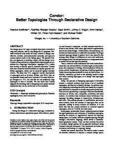
target, denoted by Ri,s ). The resource target for each task may also change over time with changing traffic. The key challenge is to quickly converge to Ri,s (t); the longer ri,s (t) is below the target, the less the task’s satisfaction. Because Ri,s is unknown and time-varying, at each allocation epoch, the allocator iteratively increases or decreases ri,s (t) in steps based on the overall accuracy (calculated in the previous epoch) to reach the right amount of resources. The size of the step determines the convergence time of the algorithm and its stability. If the step is too small, it can take a long time to move resources from a rich task to a poor one; on the other hand, larger allocation step sizes enable faster convergence, but can induce oscillations. For example, if a satisfied task needs 8 TCAMs on a switch and has 10, removing 8 TCAMs can easily drop its accuracy to zero. Intuitively, for stability, DREAM should use larger step sizes when the task is far away from Ri,s (t), and smaller step sizes when it is close. Since Ri,s is unknown, DREAM estimates it by determining when a task changes its status (from poor to rich or from rich to poor) as a result of a resource change. Concretely, DREAM’s resource allocation algorithm works as follows. At each measurement epoch, DREAM computes the sum of the step sizes of all the poor tasks sP , and the sum of the step sizes of all the rich tasks sR .4 If sP ≤ sR , then each rich task’s ri,s is reduced by its step size, and each poor task’s ri,s is increased in proportion to its step size (i.e., sR is distributed proportionally to the step size of each poor task). The converse happens when sP > sR . If we increase or decrease ri,s during one allocation epoch, and this does not change the task’s rich/poor status in the next epoch, then, we increase the step size to enable the task to converge faster to its desired accuracy. However, if the status of task changes as a result of a resource change, we return TCAM resources (but use a smaller step size) to converge to Ri,s . Figure 4 illustrates the convergence time to Ri,s (t) for different increase/decrease policies for the step size. Here, multiplicative (M) policies change step size by a factor of 2, and additive (A) policies change step size by 4 TCAM counters every epoch. We ran this experiment with other values and the results for those values are qualitatively similar. Additive increase in AM and AA has slow convergence when Ri,s (t) changes since it takes a long time to increase the step size. Although MA reaches the goal fast, it takes long for it to decrease the step size and converge to the goal. Therefore, we use multiplicative increase and decrease (MM) for changing the step size; we have also experimentally verified its superior performance. As an aside, note that our problem is subtly different from fair bandwidth allocation (e.g., as in TCP). In our setting, different tasks can have different Ri,s , and the goal is to keep their allocated resources, ri,s , above Ri,s for more tasks, but fairness is a non-goal. By contrast, TCP attempts to converge to a target fair rate that depends upon the bottleneck bandwidth. Therefore, some of the intuitions about TCP’s control laws do not apply in our setting. In the language of TCP, our approach is closest to AIAD, since our step size is independent of ri,s . In contrast to AIAD, we use large steps when ri,s is far from Ri,s for fast convergence, and we use small step sizes otherwise for saving resources by making ri,s close to Ri,s .

1000

Goal MM AM AA MA

500

0 0

100

200 300 400 500 Time(s) Figure 4: Comparing step updates algorithms

headroom is below a target value on any switch for the task. This permits the system to absorb fluctuations in total resource usage, while ensuring high task satisfaction. However, because it is impossible to predict traffic variability, DREAM may infrequently drop tasks when headroom is insufficient.5 In our current design, operators can specify a drop priority for tasks. DREAM lets the poor tasks with low drop priority (i.e., those that should be dropped last) steal resources from those tasks with high drop priority (i.e., those that can be dropped first). When tasks with high drop priority get fewer and fewer resources on some switches, and remain poor for several consecutive epochs, DREAM drops them, to ensure that they release resources on all switches. DREAM does not literally maintain a pool of unused TCAM counters as headroom. Rather, it always allocates enough TCAM counters to all tasks to maximize accuracy in the presence of traffic changes, but then calculates effective headroom when a new task arrives. One estimate of effective headroom is sR − sP (the sum of the step sizes of the rich tasks minus that of the poor tasks). However, this can under-estimate headroom: a rich task may have more resources than it needs, but its step size may have converged to a small value and may not accurately reflect how many resources it can give up while still maintaining accuracy. Hence, DREAM introduces a phantom task on each switch whose resource requirement is equal to the headroom. Rich tasks are forced to give up resources to this phantom task, but, when a task becomes poor due to traffic changes, it can steal resources from this phantom task (this is possible because the phantom task is assigned the lowest drop priority). In this case, if r ph is the phantom task’s resources, the effective headroom is r ph + sR − sP , and DREAM uses this to determine if the new task should be admitted.

5.

TASK OBJECTS AND ACCURACY ESTIMATION

In DREAM, task objects implement individual task instances. We begin by describing a generic algorithm that captures task object functionality. An important component of this algorithm is a task-independent iterative algorithm for configuring TCAM counters across multiple switches. This algorithm leverages TCAM properties, and does not depend upon details of each task type (i.e., HH, HHH or CD). We conclude the section with a discussion of the task-dependent components of the generic algorithm, such as the accuracy estimator. This deliberate separation of functionality between generic, taskindependent, and task dependent parts enables easier evolution of DREAM. To introduce a new task type, it suffices to design new algorithms for the task-dependent portion, of which the most complicated is the accuracy estimator. 5 Here, we assume that perimeter defenses are employed (e.g., as in data centers), so malicious traffic cannot trigger task drops. In future work, we plan to explore robustness to attack traffic.

Algorithm 1: DREAM task object implementation 1 foreach measurement iteration do 2 counters=fetchCounters(switches); 3 report = createReport(counters); 4 (global, locals) = t.estimateAccuracy(report, counters); 5 allocations = allocator.getAllocations(global, locals); 6 counters = configureCounters(counters, allocations); 7 saveCounters(counters,switches); 8 end

5.1

A Generic Algorithm for Task Objects

A DREAM task object implements Algorithm 1; each task object runs on the SDN controller. This algorithm description is generic and serves as a design pattern for any task object independent of the specific functionality it might implement (e.g., HH, HHH or CD). Each newly admitted task is initially allocated one counter to monitor the prefix defined by the task’s flow filter (Section 3). Task object structure is simple: at each measurement interval, a task object performs six steps. It fetches counters from switches (line 2), creates the report of task (line 3) and estimates its accuracy (line 4). Then, it invokes the per-switch allocator (line 5, Section 4) and allows the task to update its counters to match allocations and to improve its accuracy (line 6). Finally, the task object installs the new counters (line 7). Of these six steps, one of them configureCounters() can be made task-independent. This step relies on the capabilities of TCAMs alone and not on details of how these counters are used to measure HHs, HHHs or significant changes. Two other steps are task-dependent: createReport, and estimateAccuracy.

5.2

Configuring Counters for TCAMs

Overview. After the resource allocator assigns TCAM counters to each task object on each switch, the tasks must decide how to configure those counters, namely which traffic aggregates to monitor on which switch using those counters (configureCounters() in Algorithm 1). A measurement task cannot monitor every flow in the network because, in general, it will not have enough TCAM counters allocated to it. Instead, it can measure traffic aggregates, trading off some accuracy. For example, TCAM-based measurement tasks can count traffic matching a traffic aggregate expressed as a wild-card rule (e.g., traffic matching an IP prefix). The challenge then becomes choosing the right set of prefixes to monitor for a sufficiently accurate measurement while bounding resource usage. A task-independent iterative approach works as follows. It starts by measuring an initial set of prefixes in the prefix trie for the packet header field (source or destination IP) that is an input parameter to our tasks. Figure 5 shows an example prefix trie for four bits. Then, if the count on one of the monitored prefixes is “interesting” from the perspective of the specific task (e.g., it reveals the possibility of heavy hitters within the prefix), it divides that prefix to monitor its children and use more counters. Conversely, if some prefixes are “uninteresting”, it merges them to free counters for more useful measurements. While this approach is task-independent, it depends upon a taskdependent component: a prefix score that estimates how “interesting” the prefix is for the specific task. Finally, DREAM can only measure network phenomena that last long enough for this iterative approach to complete (usually, on the order of several seconds). Divide-and-Merge. Algorithm 2 describes this divide-and-merge algorithm in detail. The input to this algorithm includes (a) the current configuration of counters allocated to the task and (b) the new resource allocation. The output of this algorithm is a new configu-

Figure 5: A prefix trie of source IPs where the number on each node shows the bandwidth used by the associated IP prefix in Mb in an epoch. With threshold 10, the nodes in double circles are heavy hitters and the nodes with shaded background are hierarchical heavy hitters.

ration describing the prefixes to be monitored in the next measurement interval. In the first step, the algorithm invokes a task-dependent function that returns the score associated with each prefix currently being monitored by the task object (line 1). We describe prefix scoring later in this section, but scores are non-negative, and the cost of merging a set of prefixes is the sum of their score. Now, if the new TCAM counter allocation at some switches is lower than the current allocation (we say that these switches are overloaded), the algorithm needs to find prefixes to merge. It iteratively finds a set of prefixes with minimum cost that can be merged into their ancestors, thereby freeing entries on overloaded switches (lines 2-4). We describe how to find such candidate prefixes (cover() function) below. After merging, the score of the new counter will be the total score of merged counters. Next, the algorithm iteratively divides and merges (lines 5-16). First, it picks the counter with maximum score to divide (line 6) and determines if that results in overloaded switches, designated by the set F (line 7). If F is empty, for example, because the resource allocator increased the allocation on all switches, no merge is necessary, so the merge cost is zero. Otherwise, we use the cover() function to find the counters to merge (line 10). Next, if the score of the counter is worth the cost, we apply divide and merge (lines 12-15). After dividing, the score of children will be half of the parent’s score [42]. The algorithm loops over all counters until no other counter is worth dividing. A similar algorithm has been used for individual measurement tasks (e.g., HH [26], HHH [31], and traffic changes [41]). In this paper, we provide a general task-independent algorithm, ensuring that the algorithm uses bounded resources and adapting to resource changes on multiple switches.

Algorithm 2: Divide and Merge 1 2 3 4 5 6 7 8 9 10 11 12 13 14 15 16

computeScores(counters); while F = {over-allocated switches} 6= Φ do merge(cover(F, counters, allocations)); end repeat m = maxIndex(counters.score); F = toFree(m, allocations); solution.cost=0; if F 6= Φ then solution=cover(F, counters, allocations); end if solution.cost
On multiple switches. We now explain how divide-and-merge works across multiple switches. We consider tasks that measure phenomena on a single packet header field, and we leave to future work extensions to multiple fields. For ease of exposition, we describe our approach assuming that the user specifies the source IP field for a given task. We also assume that we know the ingress switches for each prefix that a task wishes to monitor; then to monitor the prefix, the task must install a counter on all of its ingress switches and later sum the resulting volumes at the controller. Dividing a prefix may need an additional entry on multiple switches. Formally, if two sibling nodes in the prefix trie, A and B, have traffic on switch sets SA and SB , monitoring A and B needs one entry on each switch in SA and one on each switch in SB , but monitoring the parent P needs one entry on SP = SA ∪ SB switches. Therefore, merging A and B and monitoring the parent prefix frees one entry on SA ∩ SB . Conversely, dividing the parent prefix needs one additional entry on switches in SA ∩ SB . For example, suppose that S0000 = {1, 2} and S0001 = {2, 3} in Figure 5 where set elements are switch ids. Merging S0000 and S0001 saves an entry on 2. The challenge is that we may need to merge more than two sibling prefixes to their ancestor prefix to free an entry in a switch. For example, suppose that S0010 = {3, 4} and S0011 = {4, 1}. To free an entry on switch 3, we must merge S0001 and S0010 . Therefore, we merge all four counters to their common ancestor 00 ∗ ∗. 6 To generalize, suppose that for each internal node j in the prefix trie (ancestor of counters), we know that merging all its descendant counters would free entries on a set of switches, say T j . Furthermore, let the cost for node j be the sum of the scores of the descendant monitored prefixes of j. The function cover() picks those T j sets that cover the set of switches requiring additional entries, F, with minimum total cost. There are fast greedy approximation algorithms for Minimum Subset Cover [36]. Finally, we describe how to compute T j for each internal node. For each node j, we keep two sets of switches, S j and T j . S j contains the switches that have traffic on j and is simply S jle f t ∪ S jright when j has two children jle f t , jright . T j contains the switches that will free at least one entry if we merge all its descendant counters to j. Defining it recursively, T j includes T jle f t and T jright , and contains (by the reasoning described above) the common entries between the switches having traffic on the left and right children, S jle f t ∩ S jright . T j is empty for prefixes currently being monitored.

5.3

Task-Dependent Algorithms

Beyond these task-independent algorithms, each task object implements three task-dependent algorithms. We present the taskdependent algorithms for HH, HHH, and CD tasks. A key taskdependent component is accuracy estimation, and we consider two task accuracy metrics: precision, the fraction of retrieved items that are true positives; and recall, the fraction of true positives that are retrieved. For these definitions, an item refers to a HH, HHH or change detection. Depending on the type of measurement task, DREAM estimates one of these accuracy measures to determine TCAM resource allocation. The task-dependent algorithms for these tasks are summarized in Table 1, but we discuss some of the non-trivial algorithms below. Heavy hitters: A heavy hitter is a traffic aggregate that exceeds a specified volume. For example, we can define heavy hitters as the source IPs whose traffic exceeds a threshold θ over a measurement epoch. Figure 5 shows an example of bandwidth usage for each IP prefix during an epoch. With a threshold of θ = 10Mb, there are a 6 Although we could just merge those two to 00 ∗ ∗, this creates overlapping counters that makes the algorithm more complex and adds delay in saving rules at switches.

Task HH

HHH

CD

Create report Report exact counters with volume > θ Traverse prefix trie bottomup and report a prefix h if volumeh − ∑i volumei > θ where i is a descendant detected HHH of h [15] Report exact counters with |volume − mean| > θ

Estimate accuracy Estimate recall by estimating missed HHs

Score volume #wildcards+1

Estimate precision by finding if a detected HHH is a true one

volume

Estimate recall by estimating missed changes

|volume−mean| #wildcards+1

Table 1: Task dependent methods total of two leaf heavy-hitters shown in double circles. Our divideand-merge approach iteratively drills-down to these two leaves. Accuracy Estimation: For our TCAM-based algorithm, all detected HHs are true, which means the precision is always one in this algorithm. For this reason, we use recall as a measure of accuracy for HH detection. Doing so requires an estimate of the number of true HHs the algorithm misses. We use the smaller of the following two bounds to estimate the missed heavy hitters under a non-exact prefix. First, a prefix with b wildcard bits cannot miss more than 2b heavy hitters. For example, prefix 0 ∗ ∗∗ in Figure 5 has 8 heavy hitters at most. Second, if the volume of the prefix is v, there can only be b θv c missed heavy hitters. This bound for prefix 0 ∗ ∗∗ will be 4. Finally, we need to estimate both local and global recall (Section 4). We compute the local recall for a switch based on detected HHs, and we estimate missed HHs from prefixes that have traffic on the switch. However, there are cases where only a subset of switches are bottlenecked (i.e., they have used all available counters, so it is not possible to further divide prefixes). In this case, we only consider missed HHs on these switches. Hierarchical heavy hitters: A variant of heavy hitters, called Hierarchical Heavy Hitters (HHHs) [15] is useful for anomaly detection [42] and DDoS detection [33]. A HHH is (recursively) defined by the longest IP prefixes that contribute traffic exceeding a threshold θ of total traffic, after excluding any HHH descendants in the prefix trie. For example in Figure 5, prefix 010* is a HHH as IPs 0100 and 0101 collectively have large traffic, but prefix 01** is not a HHH because excluding descendent HHHs (010* and 0111), its traffic is less than the threshold. Accuracy Estimation: For HHHs, our algorithm estimates precision by determining whether a detected HHH is a true positive or a false positive. Our algorithm assigns a precision value to each detected HHH: the value is either 0 if it is a false positive, 1 if a true positive, or fractional if there is ambiguity in the determination, as discussed below. The overall accuracy estimate is an average of these values. The method for making these value assessments is different for HHHs without and with detected descendant HHHs. If a detected HHH h has no detected descendant HHHs (e.g., 0000, 010*, 0111 in Figure 5), it is a false positive HHH if it has been detected instead of one of its descendants. So, for it to be a true positive HHH, we need to ensure that none of its descendants could have been a HHH. There are three cases. (1) h is an exact IP. (2) We monitored the descendants of h and their volume is below the threshold θ . For example, if we monitor 0100 and 0101, we can confirm that the detected HHH 010* is a true one. In these two cases, it is easy to tell h is a true HHH. (3) We only monitored h and do not know about its descendants. If h has a count larger than 2θ , then h cannot be a true HHH, because the volume of at least one of its children must be above θ . If the volume is smaller than 2θ , either the detected prefix or one of its sub-prefixes is HHH, so we set its precision value to 0.5. For an HHH h with detected descendant HHHs, the error in the detected descendant HHHs can make h a false HHH. For example

in Figure 5, suppose that we report 0000, 010* and 011* as HHHs. Now, the volume for 0*** excluding descendant HHHs will be 8 because of false detection of 011*. Therefore, instead of 0***, we detect **** as HHH. In this scenario, we have over-approximated the traffic from descendant HHHs of ****. In the worst case, the over-approximated traffic has been excluded from a child of the detected HHH. Thus, for each child prefix, we find if adding up these over-approximations could make them a HHH. If any child with a new volume becomes HHH, the parent cannot be, so as a heuristic, we halve the precision weight of h. The over-approximation for a HHH confirmed to be true is 0, and the over-approximation for other HHHs can be at most volume − θ . The global precision is the average precision value of detected HHHs. To compute the local precision per switch, we compute the average precision value of HHH prefixes from each switch. If a HHH has traffic from multiple switches, we give the computed precision value only to bottleneck switches, and precision 1 to other switches. For HHH tasks, recall can be calculated similar to HH tasks. We have experimentally found that, for HHH, recall is correlated with precision. Change detection: A simple way to define the traffic change of a prefix is to check if the difference between its current volume and a moving average of its volume exceeds a specified threshold. In this sense, change detection is similar to HH detection: a change is significant if |volume − mean| > θ . Thus, for change detection, reporting, prefix scoring, and accuracy estimation are similar to those for HH tasks (Table 1): wherever volume is used in HH tasks, |volume − mean| is used for CD.

6.

EVALUATION

We have implemented a complete prototype of DREAM, and use this to evaluate our approach and compare it with alternatives. We then use simulations to explore the performance of DREAM on larger networks, and also study its parameter sensitivity.

6.1

Evaluation Methodology

DREAM Implementation: We have implemented the DREAM resource allocator and the task objects in Java on the Floodlight controller [4]. Our implementation interfaces both with hardware OpenFlow switches, and with Open vSwitch [5]. We have also implemented alternative resource allocation strategies, described below. Our total implementation is nearly 20,000 lines of code. DREAM Parameter Settings: We use a one second measurement interval and a two second allocation interval. We set the headroom to 5% of the switch capacity and drop tasks if their global accuracy is below the bound for 6 consecutive allocation iterations. The sensitivity of DREAM to these parameters is explored in Section 6.4.

Tasks: Our workload consists of the three types of tasks, HH, HHH and CD, both individually and in combination. We choose 80% as the default accuracy bound for all tasks since we have empirically observed that to be the point of diminishing returns for many tasks, but also explore DREAM’s performance for other choices of accuracy bounds. We smooth the local and global accuracies using EWMA with history weight of α = 0.4. The flow filters for the tasks are chosen randomly from prefixes with 12 wildcard bits to fit all our tasks. The default threshold for the above tasks is 8Mb, and for change detection we also use the history weight of α = 0.8. Our default drop priority is to drop the most recent task first.

By controlling the mapping of prefixes to switches, we create different scenarios of tasks on switches. For example, a tenant can own a subnet of /12, and its virtual machines in this subnet can be located on different switches. If we assign multiple /10 prefixes to switches (i.e., each switch sees traffic from many tenants), each task will have traffic from one switch. However, if we assign /15 prefixes to switches (i.e., one tenant sends traffic from many switches), each task monitors traffic from 8 switches at most. Tasks run for an average of 5 minutes. For evaluations on our prototype, 256 tasks having traffic from 8 switches arrive based on a Poisson process during 20 minutes. For the large-scale simulation, 4096 tasks having traffic from 8 out of 32 switches arrive during 80 minutes. We note that these are fairly adversarial settings for task dynamics, and are designed to stress test DREAM and other alternatives. Finally, we use a 5-hour CAIDA packet trace [3] from a 10Gbps link with an average 2Gbps load. We divide it into 5-min chunks, each of which contains 16 /4 prefixes, of which only prefixes with >1% total traffic are used. Each task randomly picks a /4 prefix which is mapped to its /12 filter Evaluation metrics: We evaluate DREAM and other alternatives using three metrics. The satisfaction of a task is the percentage of time a task has an accuracy above the bound when the task was active. In results from our prototype, we use estimated accuracy because delays in installing TCAM counters in the actual experiment make it difficult for us to assess the ground-truth in the traffic seen by a switch. We have found in our evaluations that the estimated accuracy consistently under-estimates the real accuracy by 5-10% on average, so our prototype results are a conservative estimate of the actual satisfaction that tasks would see in practice. In our simulation results, we use the real accuracy. We show both the average and 5th percentile for this metric over all tasks. The latter metric captures the tail behavior of resource allocation: a 5-th percentile of 20 means that 95% of tasks had an accuracy above the bound for 20% of their lifetime. The drop and rejection ratios measure the percentage of tasks that are dropped and rejected, respectively. While the rejection ratios can be a function of the workload and can be high in highly overloaded conditions, we expect drop ratios to be small for a viable scheme (i.e., it is desirable that a task, once admitted, is not dropped, but may be rejected before admission). Alternative Strategies: One alternative we explore is to reserve a Fixed fraction of counters on each switch for a task, and reject tasks for which this fixed allocation cannot be made. While we evaluated fixed allocation with different fractions, here we only show the re1 of the resources on a switch sults for the scenario that allocates 32 per task. Larger allocations result in higher satisfaction for fewer tasks and a higher rejection ratio, and smaller fixed allocations accept more tasks at the expense of lower satisfaction. A more complex algorithm is to give Equal amounts of resources to each task. When a task joins, it gets an equal share of counters as other tasks on the switches it has traffic from. The allocations are also updated when a task leaves, and Equal does not reject tasks. Experimental setup: We replay the CAIDA traffic on 8 switches. We attempted to evaluate DREAM on a modern hardware switch (the Pica8 3290 [6]) but its delay for rule installation is unacceptably high: 256 rules take 1 second, and 512 rules take 10 seconds. We believe better engineering will result in improved installation times in the future; indeed, for applications with tight control loops like ours, it is essential to improve installation times in hardware switches. Our evaluations are conducted on software switches [5] that can delete and save 512 rules in less than 20ms. We also reduce

100

80

80

40

0

Results from Prototype

Large capacity switches. For large switches, DREAM can keep almost all tasks satisfied by temporally and spatially multiplexing TCAM resources without rejecting or dropping any task (Figure 7). For example, Figure 6(b) shows that 95% of tasks were satisfied for more than 94% of their lifetime. By contrast, a high mean and a dramatically lower 5th percentile (about 40%, or nearly 2× less than DREAM) for Equal indicate that this scheme has undesirable tail behavior: it keeps tasks that require fewer resources satisfied, but leaves large tasks unsatisfied. This is undesirable in general: larger tasks are where the action happens, in a manner of speaking, and cannot be left dissatisfied. The Fixed approach achieves high average satisfaction, but has two drawbacks: poor tail performance, and a high rejection ratio of about 30%. Highly resource-constrained switches. For smaller switches, where our workload overloads the resources on switches, DREAM leverages rejection to limit the load and keep active tasks satisfied by multiplexing resources. For example, in Figure 6(a) for a switch with 512 counters, DREAM rejects about 50% of tasks, but can keep 95% of tasks satisfied for more than 70% of their lifetime. By contrast, in this setting, Equal performs pathologically worse: its average satisfaction is 20% and 5% of tasks under Equal get nearly zero satisfaction. This is because Equal does not perform admission control and it under-provisions resources in small switches and thus gets low satisfaction. We emphasize that this is an adversarial workload and represents a high degree of overload: DREAM has to reject nearly 50% of the tasks, and drop about 10% in order to satisfy the remaining tasks. Also, DREAM’s mean and 5th percentile satisfaction is a little lower than for the larger switch capacity case, mostly because the adaptation required to fit tasks into the smaller switch requires more allocation epochs to converge. Across different task types, the results are qualitatively consistent, save for two exceptions. First, the drop ratio for HH detection (Figure 7(a)) increases from switch capacity of 512 to 1024, which is likely because of a decrease in the rejection ratio. Moreover, its drop rate is higher than other tasks, which we believe is because we under-estimate the accuracy of tasks. Remember that to calculate the number of missed HHs under a prefix we used the bound of volume θ . However, the missed HHs could have larger volumes than θ and make this upper bound loose. This loose upper bound ensures better 5th percentile performance than other schemes we have tried, so it seems a better design choice: it drops more tasks to favor satisfying more. Second, the average satisfaction of Equal and Fixed is higher than other task types for change detection (but the tail performance is poor). This is because, in our dataset, not all epochs have a significant change, thus the tasks are satisfied in those epochs even with very small resources.

DREAM−reject Fixed−reject DREAM−drop

60 40 20

512

1024 2048 Switch capacity

0 512

4096

(a) Satisfaction

1024 2048 Switch capacity

4096

(b) Rejection and drop

Figure 8: Large scale simulation (combined workload) 100

100

80

80 % of tasks

Figure 6 shows, for different switch capacities, the 5th percentile and mean satisfaction of tasks for HHH, HH, and CD separately, as well as a combined workload that runs a mixture of these tasks. The mean value is the upper end of each vertical bar, and the 5th percentile is the lower end. These figures demonstrate DREAM’s superior performance compared to the alternatives, both in terms of the mean and the 5th percentile.

DREAM Equal Fixed

60

% of tasks

100

20

Satisfaction

6.2

Satisfaction

control loop delay by using incremental update of TCAM counters and associated rules, updating at each epoch only the rules that have changed from the previous epoch. We show below that this strategy results in acceptable rule installation performance (Section 6.5). In our experiments, the DREAM prototype runs on a Floodlight controller [4] on a quad core 2.4 Ghz Xeon processor connected to the switches through a 1Gbps shared link with ping delay of 0.25ms.

60 40 DREAM Equal Fixed

20 0

60

70 80 Accuracy bound

(a) Satisfaction

DREAM−reject Fixed−reject DREAM−drop

60 40 20

90

0

60

70 80 Accuracy bound

90

(b) Rejection and drop

Figure 9: Accuracy bound paramter sensitivity analysis

6.3

Results from Simulation at Scale

We use simulation to study the performance of DREAM and other alternatives at larger scale. Our simulator uses the same code base as the prototype and is validated for the same setting [32]. DREAM’s superior performance is also evident in larger networks. Figure 8 compares the satisfaction and rejection ratio of the combined workload on 32 switches with 4096 tasks (results for individual task types are quantitatively similar). In this much larger setting, the superior tail satisfaction of DREAM at low load (high capacity) and the superior average satisfaction at high load (low capacity) are strikingly evident. As with smaller networks, DREAM has a small drop ratio (less than 5%) at high load.

6.4

Parameter Sensitivity Analysis

To understand how sensitive our results are to changes in various parameters, we conduct several experiments with a switch capacity of 1024 TCAM entries, but vary several other parameters. We note that for our baseline workload, 1024 TCAM entries represent a constrained setting. For this set of results, we show results for a specific type of task (HHH), rather than using results from a combined workload, as this makes it easier to interpret the results (Figures 9). A companion report [32] evaluates sensitivity to HHH threshold, number of switches per task, task duration and task arrival rate. The qualitative behavior of other tasks is similar. DREAM keeps tasks satisfied for different accuracy bounds. With higher accuracy bounds the allocation becomes harder, since tasks in general need more resources, but DREAM can keep more tasks satisfied with a smaller rejection rate compared to Fixed allocation (Figure 9). DREAM is also uniformly better than Equal allocation because it effectively multiplexes resources across tasks.

Headroom is important to keep drop rate low. If DREAM does not reject tasks a priori, many tasks will starve just after joining the system. For example, Figure 10(b) shows a drop rate of 30% for DREAM when there is no headroom at an allocation interval of 2s. Interestingly, the level of headroom does not seem to make a significant difference in the statistics of satisfaction, but can affect drop rates. With a 5% and 10% headroom, drop rates are negligible. Other DREAM parameters include allocation interval, drop threshold, and the MM algorithm multiplicative factor. Figure 10(a) shows

100

60 5th %

40

DREAM Equal Fixed

20 0

512

1024 2048 Switch capacity

DREAM Equal Fixed

60 40

Satisfaction

80 Satisfaction

Satisfaction

80

20 0

4096

100

100

80

80

60 40 DREAM Equal Fixed

20

512

(a) HH

1024 2048 Switch capacity

0

4096

512

(b) HHH

1024 2048 Switch capacity

Satisfaction

Mean

100

60 40 DREAM Equal Fixed

20 0

4096

(c) CD

512

1024 2048 Switch capacity

4096

(d) Combined workload

Figure 6: Satisfaction in prototype 100

60 40

60 40

20

20

0 512

1024 2048 Switch capacity

(a) HH

60 40

1024 2048 Switch capacity

4096

0 512

(b) HHH

100

None−drop 1%−drop 5%−drop 10%−drop

60

% of tasks

Satisfaction

80

1024 2048 Switch capacity

4096

(c) CD

40

None−reject 1%−reject 5%−reject 10%−reject

60 40 20

None 1% 5% 10%

20

2

4 8 Allocation epoch (s)

16

(a) Satisfaction

0

2

4 8 Allocation epoch (s)

16

(b) Rejection and drop

Figure 10: Headroom and allocation epoch (combined workload)

6.5

Control Loop Delay

The delay of the control loop – the process of configuring counters and updating rules in TCAMs – can affect the accuracy of real prototypes because important events can be missed while these counters are being updated. We calculate the control loop delay by calculating the average delay between fetching the counters from the switches to receiving the OpenFlow barrier reply from all switches after installing incremental rules on the prototype. Figure 11(a) breaks down the delay of control loop into: saving the incremental rules, fetching the counters, allocating resources, creating the report and estimating its accuracy, configuring counters through divide and merge algorithm and the runtime overhead for combining counter statistics from multiple switches and creating a counter on multiple switches for all tasks. The interesting points are: (1) the allocation delay (the overhead of computing new allocations) is negligible compared to other delays; (2) the average (95th %) allocation delay decreases with increasing switch size from 0.65 (3.1) ms to 0.5 (1.3) ms, because for larger switches, fewer tasks are dissatisfied although more tasks have been admit-

60 40 20

Figure 7: Rejection and drop in prototype that allocating resources infrequently with a larger allocation interval results in lower satisfaction because DREAM cannot adapt resources quickly enough. Smaller drop threshold increases the drop rate and satisfaction, and increasing the multiplicative factor of the MM algorithm causes higher rejection rate because poor tasks overshoot their goal by large change step sizes and thereby reduce headroom. Note that a smaller multiplication factor requires a larger drop threshold to avoid unnecessary drops in under-loaded cases. (a) Prototype delay 80

DREAM−reject Fixed−reject DREAM−drop

80

20

0 512

4096

100 DREAM−reject Fixed−reject DREAM−drop

80 % of tasks

% of tasks

% of tasks

100 DREAM−reject Fixed−reject DREAM−drop

80

% of tasks

DREAM−reject Fixed−reject DREAM−drop

80

0 512

1024 2048 Switch capacity

4096

(d) Combined workload

30 Allocation delay (ms)

100

20

10

0 2 4

8

16 Switch per task

32

(b) Allocation delay

Figure 11: Control loop delay (combined workload) ted; (3) fetch times dominate save times (although it takes longer to save or delete a counter than to fetch one) because we fetch all counters, but only delete and save incrementally. For example, for the case of switches with 1024 TCAM capacity, on average in each epoch 90% of the counters did not change. This number increases for larger switch capacities as tasks need to configure their counters less frequently because (a) they already have an accurate view of network (b) their allocations changes rarely as more tasks are satisfied with more resources. Finally, the DREAM controller scales to many tasks because it is highly parallelizable; each task can run on a core and each perswitch allocator can run separately. The per-switch resource allocator does more work as we increase the number of switches per task, since each switch sees more tasks. Figure 11(b) shows that the mean, and 95th percentile of allocation delay in the large scale simulation environment (on a 32 core machine) increases for larger number of switches per task, but the mean is still less than 10ms and the control loop delay is still dominated by other (unavoidable) latencies in the system.

7.

RELATED WORK

Software-defined measurement and programmable measurement: Prior work has explored different measurement primitives [20, 35], but, unlike DREAM, assumes offline analysis of collected measurement data, and thus cannot dynamically change their measurement resource usage when traffic changes or more measurement tasks come. Previous work on software-defined measurement [39, 31, 25] and programmable measurement [18, 40] has shown the benefits of

allowing operators or cloud tenants to customize the measurement for their traffic with different measurement primitives. Amazon CloudWatch [2] also provides simple customized measurement interface for tenants. Like these, DREAM allows measurement tasks to specify the flows and traffic characteristics to measure, but, beyond prior work, provides dynamic resource allocation solutions to enable more and finer-grained measurement tasks. Resource allocation of measurement tasks: OpenSketch [39] uses worst case theoretical bounds of sketches to allocate resources on a single switch to measurement tasks. CSAMP [34] uses consistent sampling to distribute flow measurement on multiple switches for a single measurement task and aims at maximizing the flow coverage. Volley [29] uses a sampling-based approach to monitor state changes in the network, with the goal of minimizing the number of sampling operations. Payless [14] decides the measurement frequency for concurrent measurement tasks to minimize the controller bandwidth usage, but does not provide any guarantee on accuracy or bound on switch resources. In contrast, DREAM focuses on flow-based rules in TCAM. DREAM dynamically allocates network-wide resources to multiple measurement tasks to achieve their given accuracy bound. TCAM-based measurement and accuracy estimators: Previous TCAM-based algorithms for specific measurement tasks either only work on a single switch [31, 26, 25] or do not adjust counters for bounded resources at switches [41, 26]. We designed a generic divide-and-merge measurement framework for multiple switches with resource constraints. Previous work has proved the theoretical bounds for the worst case resource usage for only hash-based measurements [17, 16]. We proposed heuristics for estimating the accuracy of TCAM-based measurement algorithms by exploiting relationships between counters already collected.

8.

CONCLUSIONS Measurement is fundamental for network management systems.

DREAM enables operators and cloud tenants to flexibly specify

their measurement tasks in a network, and dynamically allocates TCAM resources to these tasks based on the resource-accuracy tradeoffs for each task. DREAM ensures high accuracy for tasks, while taking network-wide resource constraints as well as traffic and task dynamics into account.

9.

ACKNOWLEDGEMENTS

We thank our shepherd Rodrigo Fonseca and SIGCOMM reviewers for their helpful feedback. This paper is partially supported by Software R&D Center at Samsung Electronics, Cisco, Google, and USC Zumberge.

10.

REFERENCES

[1] http://news.netcraft.com/archives/2013/05/20/amazonweb-services-growth-unrelenting.html. [2] Amazon CloudWatch. http://aws.amazon.com/cloudwatch/. [3] CAIDA Anonymized Internet Traces 2012. http://www.caida.org/ data/passive/passive_2012_dataset.xml. [4] Floodlight. http://www.projectfloodlight.org/floodlight/. [5] Open vSwitch. http://openvswitch.org/. [6] Pica8 P-3290 switch. http://www.pica8.com/documents/pica8datasheet-48x1gbe-p3290-p3295.pdf. [7] M. Al-Fares, S. Radhakrishnan, B. Raghavan, N. Huang, and A. Vahdat. Hedera: Dynamic Flow Scheduling for Data Center Networks. In NSDI, 2010. [8] M. Alizadeh, S. Yang, M. Sharif, S. Katti, N. McKeown, B. Prabhakar, and S. Shenker. pFabric: Minimal Near-optimal Datacenter Transport. In SIGCOMM, 2013. [9] A. M. Azab, P. Ning, and X. Zhang. SICE: A Hardware-level Strongly Isolated Computing Environment for x86 Multi-core Platforms. In CCS, 2011. [10] H. Ballani, P. Costa, T. Karagiannis, and A. I. Rowstron. Towards Predictable Datacenter Networks. In SIGCOMM, 2011.

[11] T. Benson, A. Anand, A. Akella, and M. Zhang. MicroTE: Fine Grained Traffic Engineering for Data Centers. In CoNEXT, 2011. [12] K. Chen, A. Singla, A. Singh, K. Ramachandran, L. Xu, Y. Zhang, X. Wen, and Y. Chen. OSA: An Optical Switching Architecture for Data Center Networks With Unprecedented Flexibility. In NSDI, 2012. [13] Y. Chen, R. Griffith, J. Liu, R. H. Katz, and A. D. Joseph. Understanding TCP Incast Throughput Collapse in Datacenter Networks. In WREN, 2009. [14] S. R. Chowdhury, M. F. Bari, R. Ahmed, and R. Boutaba. PayLess: A Low Cost Network Monitoring Framework for Software Defined Networks. In IEEE/IFIP NOMS, 2014. [15] G. Cormode, F. Korn, S. Muthukrishnan, and D. Srivastava. Finding Hierarchical Heavy Hitters in Data Streams. In VLDB, 2003. [16] G. Cormode and S. Muthukrishnan. An Improved Data Stream Summary: The Count-Min Sketch and its Applications. Journal of Algorithms, 55(1), 2005. [17] G. Cormode and S. Muthukrishnan. Summarizing and Mining Skewed Data Streams. In SIAM Conference on Data Mining (SDM), 2005. [18] C. Cranor, T. Johnson, O. Spataschek, and V. Shkapenyuk. Gigascope: a Stream Database for Network Applications. In SIGMOD, 2003. [19] A. Curtis, J. Mogul, J. Tourrilhes, P. Yalagandula, P. Sharma, and S. Banerjee. DevoFlow: Scaling Flow Management for High-Performance Networks. In SIGCOMM, 2011. [20] C. Estan and G. Varghese. New Directions in Traffic Measurement and Accounting. SIGCOMM Computer Communication Review, 32(4):323–336, 2002. [21] A. Feldmann, A. Greenberg, C. Lund, N. Reingold, J. Rexford, and F. True. Deriving Traffic Demands for Operational IP Networks: Methodology and Experience. Transactions on Networking, 9(3), 2001. [22] R. Gandhi, H. Liu, Y. Hu, G. Lu, J. Padhye, L. Yuan, and M. Zhang. Duet: Cloud Scale Load Balancing with Hardware and Software. In SIGCOMM, 2014. [23] D. Y. Huang, K. Yocum, and A. C. Snoeren. High-fidelity Switch Models for Software-defined Network Emulation. In HotSDN, 2013. [24] S. Jain, A. Kumar, S. Mandal, J. Ong, L. Poutievski, A. Singh, S. Venkata, J. Wanderer, J. Zhou, M. Zhu, et al. B4: Experience with a Globally-deployed Software Defined WAN. In SIGCOMM, 2013. [25] L. Jose, M. Yu, and J. Rexford. Online Measurement of Large Traffic Aggregates on Commodity Switches. In Hot-ICE, 2011. [26] F. Khan, N. Hosein, C.-N. Chuah, and S. Ghiasi. Streaming Solutions for Fine-Grained Network Traffic Measurements and Analysis. In ANCS, 2011. [27] A. Kumar, M. Sung, J. J. Xu, and J. Wang. Data Streaming Algorithms for Efficient and Accurate Estimation of Flow Size Distribution. In SIGMETRICS, 2004. [28] A. Lall, V. Sekar, M. Ogihara, J. Xu, and H. Zhang. Data Streaming Algorithms for Estimating Entropy of Network Traffic. In SIGMETRICS/Performance, 2006. [29] S. Meng, A. K. Iyengar, I. M. Rouvellou, and L. Liu. Volley: Violation Likelihood Based State Monitoring for Dataceners. ICDCS, 2013. [30] M. Mitzenmacher, T. Steinke, and J. Thaler. Hierarchical Heavy Hitters with the Space Saving Algorithm. arXiv:1102.5540, 2011. [31] M. Moshref, M. Yu, and R. Govindan. Resource/Accuracy Tradeoffs in Software-Defined Measurement. In HotSDN, 2013. [32] M. Moshref, M. Yu, R. Govindan, and A. Vahdat. DREAM: Dynamic Resource Allocation for Software-defined Measurement. Technical Report 14-945, Computer Science, USC, 2014. http://www.cs.usc.edu/assets/007/91037.pdf. [33] V. Sekar, N. G. Duffield, O. Spatscheck, J. E. van der Merwe, and H. Zhang. LADS: Large-scale Automated DDoS Detection System. In ATC, 2006. [34] V. Sekar, M. K. Reiter, W. Willinger, H. Zhang, R. R. Kompella, and D. G. Andersen. CSAMP: A System for Network-Wide Flow Monitoring. In NSDI, 2008. [35] V. Sekar, M. K. Reiter, and H. Zhang. Revisiting the Case for a Minimalist Approach for Network Flow Monitoring. In IMC, 2010. [36] V. V. Vazirani. Approximation Algorithms. Springer-Verlag New York, Inc., 2001. [37] Z. Wang and X. Jiang. Hypersafe: A Lightweight Approach to Provide Lifetime Hypervisor Control-flow Integrity. In SP, 2010. [38] D. Xie, N. Ding, Y. C. Hu, and R. Kompella. The Only Constant is Change: Incorporating Time-varying Network Reservations in Data Centers. SIGCOMM Computer Communication Review, 42(4), 2012. [39] M. Yu, L. Jose, and R. Miao. Software Defined Traffic Measurement with OpenSketch. In NSDI, 2013. [40] L. Yuan, C.-N. Chuah, and P. Mohapatra. ProgME: Towards Programmable Network MEasurement. Transactions on Networking, 19(1), 2011. [41] Y. Zhang. An Adaptive Flow Counting Method for Anomaly Detection in SDN. In CoNEXT, 2013. [42] Y. Zhang, S. Singh, S. Sen, N. Duffield, and C. Lund. Online Identification of Hierarchical Heavy Hitters: Algorithms, Evaluation, and Applications. In IMC, 2004.