DUALITY FOR FINITE HILBERT ALGEBRAS SERGIO CELANI AND LEONARDO CABRER
Abstract. In this work we shall give a characterization of the Hilbert algebras given by the order and we will prove a duality for finite Hilbert algebras by means of finite ordered sets endowed with a distinguished set of subsets. We will also study the case when the finite Hilbert algebras are join-semilattices or meet-semilattices relative to the natural order defined by the implication. Finally we will prove that Hilbert do not admit a natural duality.
1. Introduction and Preliminaries Hilbert algebras represent the algebraic counterpart of the implicative fragment of Intuitionistic Propositional Logic. In [5] A. Diego gives a topological representation for Hilbert algebras and he proves that every Hilbert algebra is isomorphic to a subalgebra of the implicative reduct of a Heyting algebra generated by a certain topological space. This result is a generalization of the known results given by M. Stone for Heyting algebras. Other representation theorem can be given by using poset. In [3] the first author of this paper proves that for every Hilbert A algebra there exists a poset hX, ≤i such that A is isomorphic to a subalgebra of the implicative reduct of the Heyting algebra Pi (X) of increasing subsets of hX, ≤i. Unfortunately, these representations do not give a full duality. However, using some results of [3] and some ideas of [4], it is possible to give a duality for the case of finite Hilbert algebras. This is the main objective of the present paper. We shall prove that the dual space of a finite Hilbert algebra A is a structure hX, ≤, Si, called Hilbert space, where hX, ≤i is a poset and S is a non-empty subset of the power set P (X). This duality is a full duality, i.e., the category of finite Hilbert algebras with homomorphisms is dually equivalent to the category of finite Hilbert spaces with adequate morphisms. In the remaining part of this section we shall review some results on Hilbert algebras and we shall introduce notations and some new definitions. In Section 2 we shall define the notion of Hilbert algebra given by the order and we will prove a characterization of this class of Hilbert algebras. In Section 3 we will give the above mentioned representation and duality for finite Hilbert algebras by means of the so-called H-spaces. In Section 4 we will introduce an important reflective subcategory of H-spaces. In Section 5 we shall study the case of finite Hilbert algebra with lattice operations, i.e., finite Hilbert algebras where the natural order defines a meet or join operation. In Section 6 we will prove that Hilbert algebras do not admit a natural duality, proving that the variety of Hilbert algebras is not generated by any finite algebra. For the rest of this paper we will use the following conventions. Given a set X and a subset Y ⊆ X we will note X\Y = {x ∈ X : x ∈ / Y }, when there is no way to confusion we will note X\Y = Y c . Given R ⊆ X × Y , we will note R (x) = {z ∈ Y : (x, z) ∈ R} and R−1 (y) = {z ∈ X : (z, y) ∈ R}. Given a poset hX, ≤i, a set Y ⊆ X is called increasing if it is closed under ≤, i.e., if for every x ∈ Y and every y ∈ X, if x ≤ y then y ∈ Y . Dually, Y ⊆ X is said to be decreasing if for every x ∈ Y and every y ∈ X, if y ≤ x then y ∈ Y . We will note= {x ∈ X : y ≤ x for some y ∈ Y } to the least increasing set that contain Y and analogously (Y ] = {x ∈ X : x ≤ y for some y ∈ Y } to the least decreasing set that contain Y . When Y = {x}, we will note [Y ) ((Y ]) by [x) ((x]). The set of all increasing subsets of X will be denoted by Pi (X), and the power set of X by P(X). Definition 1. A Hilbert algebra is an algebra A = hA, →, 1i of type (2, 0) such that the following axioms hold in A : 1991 Mathematics Subject Classification. 03G25, 06A99. Key words and phrases. Hilbert algebras, ordered sets, irreducible elements, H-spaces, meet-semilattices, joinsemilattices, Brouwerian semilattices. 1
2
SERGIO CELANI AND LEONARDO CABRER
H1. a → (b → a) = 1. H2. (a → (b → c)) → ((a → b) → (a → c)) = 1. H3. a → b = 1 = b → a imply a = b. A is called trivial if A = {1}. In [5] Diego proves that the class of Hilbert algebras form a variety which is denoted by H. In this paper the symbol ⇒ is used for logical implication, and ⇔ for logical equivalence. Lemma 2. Let A = hA, →, 1i ∈ H. Then for every a, b, c ∈ A the following assertions are satisfied: (1) a → a = 1. (2) 1 → a = a. (3) a → (b → c) = b → (a → c). (4) a → (b → c) = (a → b) → (a → c). (5) a → ((a → b) → b) = 1. (6) a → (a → b) = a → b. (7) ((a → b) → b) → b = a → b. (8) (a → b) → ((b → a) → a) = (b → a) → ((a → b) → b). It is easy to see that the binary relation ≤ defined in a Hilbert algebra A by a ≤ b if and only if a → b = 1, is a partial order on A with greatest element 1. This order is called the natural ordering on A. Example 3. Let hX, ≤i be a poset. It is easy to see that hPi (X) , 7−→, Xi is a Hilbert algebra where the implication 7−→ is defined by: U 7−→ V = {x ∈ X : [x) ∩ U ⊆ V } , for U, V ∈ Pi (X).We can see that in the definition of 7−→ is not necessary that U, V ∈ Pi (X), since U 7−→ V ∈ Pi (X), for every U, V ∈ P (X). Remark 4. Note that if hX, ≤i is a poset and x, y ∈ X, then: c
c
x ≤ y ⇔ {y} 7−→ ∅ ⊆ {x} 7−→ ∅ ⇔ ({x} 7−→ ∅] ⊆ ({y} 7−→ ∅] . Given A ∈ H and a, a1 , . . . , an ∈ A, we define: if n = 1, a1 → a (an , . . . , a1 ; a) = an → (an−1 , . . . , a1 ; a) if n > 1. Let A ∈ H. A subset D ⊆ A is a deductive system of A if 1 ∈ D, and if a, a → b ∈ D then b ∈ D. The set of all deductive systems of a Hilbert algebra A is noted Ds (A). It is easy to \ prove that Ds (A) is closed under arbitrary intersections. So, given X ⊆ A the set hXi = {D ∈ Ds (A) : X ⊆ D}, is called the deductive system generated by X. If X = {a}, then we will denote hXi = hai. Let D ∈ Ds (A). If there exists some a ∈ A such that D = hai we shall say that D is principal. The deductive system generated by a subset X ⊆ A can be characterized as the set: hXi = {a ∈ A : there exist a1 , . . . , an ∈ X such that (a1 , . . . , an ; a) = 1} . In consequence, we get that hai = {b ∈ A : a ≤ b} = [a). Let A ∈ H. Let D ∈ Ds (A) − {A}. We shall say that D is irreducible if and only if for any D1 , D2 ∈ Ds (A) such that D = D1 ∩ D2 , it follows that D = D1 or D = D2 . We shall say that DTis completely irreducible if and only if for any family {Di : i ∈ I} ⊆ Ds (A) such that D = {Di : i ∈ I}, then D = Di for some i ∈ I. The set of all irreducible (completely irreducible) deductive systems of a Hilbert Algebra A is noted Dsi (A) (Dci (A)). It is clear that Dci (A) ⊆ Dsi (A). If A is a finite Hilbert algebra, then Dci (A) = Dsi (A). For a proof of the next theorems see [5]. Theorem 5. Let A ∈ H. Let D ∈ Ds (A) − {A}. Then the following conditions are equivalent:
DUALITY FOR FINITE HILBERT ALGEBRAS
3
(1) D ∈ Dsi (A). (2) If a, b ∈ / D there exists c ∈ / D such that a, b ≤ c. (3) If a, b ∈ / D there exists c ∈ / D such that a → c, b → c ∈ D. Theorem 6. Let A ∈ H. Let D ∈ Ds (A). Then the following conditions are equivalent: (1) D ∈ Dci (A). (2) There exists a ∈ / D such that if D E ∈ Ds (A), then a ∈ E. (3) There exists a ∈ / D such that b → a ∈ D, for every b ∈ / D. Let D ∈ Ds (A) and a ∈ A. We shall say that a is associated with D or that D is maximal relative to a, if D is maximal with respect to the deductive systems which do not contain a, i.e., D is maximal in the set {E ∈ Ds (A) : a ∈ / E}. From the above theorem we can deduce the next corollary: Corollary 7. Let A ∈ H. Then the following conditions are satisfied: (1) If D ∈ Ds (A) and a ∈ / D then there exists Q ∈ Dci (A) such that a ∈ / Q (moreover, a is associated with Q) and D ⊆ Q. (2) If a, b ∈ A are such that a � b then there exists Q ∈ Dci (A) such that b ∈ / Q (moreover b is associated with Q) and a ∈ Q. Note that the previous corollary proves that for every D ∈ Ds (A) we have that: \ D= Q D⊆Q Q∈Dci (A)
Definition 8. Let A ∈ H. We define a relation KA ⊆ Dci (A) × A as follows: (D, a) ∈ KA if and only if a is associated with D. When there is no risk of ambiguity we will omit the subscript and note K instead of KA . Lemma 9. Let A ∈ H. Let D ∈ Dci (A). For each a, b ∈ K (D) there exists c ∈ A such that a ≤ c, b ≤ c and c ∈ K (D). Proof. Let a, b ∈ K (D). Since a, b ∈ / D and D is also irreducible, by theorem 5 we get that there exists c ∈ / D such that a ≤ c and b ≤ c. There exists a deductive system E associated with c such that D ⊆ E, then a ∈ / E. Then E = D because D is maximal relative to a. Thus c ∈ K (D).� Let A be Hilbert algebra. Let us consider the poset hDci (A) , ⊆i and the mapping ϕA : A → Pi (Dci (A)) defined by ϕA (a) = {P ∈ Dci (A) : a ∈ P } . For a proof of the next theorem see [5] or [3]. Theorem 10. Let A ∈ H. Then A is isomorphic to the subalgebra ϕA (A) = {ϕA (a) : a ∈ A} of hPi (Dci (A)) , 7−→, Dci (A)i. 2. Hilbert algebras given by the order In [5] A. Diego introduce the Hilbert algebras given by order. This kind of Hilbert algebras will be useful later to construct examples. In this section we will characterize the Hilbert algebras given by order by means of its deductive systems and by means of its irreducible elements. Definition 11. A Hilbert algebra A is called given by the order ≤ if and only if for every a, b ∈ A, b if a � b, a→b= 1 if a ≤ b.
4
SERGIO CELANI AND LEONARDO CABRER
Definition 12. Let A ∈ H. An element p ∈ A − {1} is called irreducible if for each a ∈ A, a ≤ p or a → p = p. In the following result we shall give an useful characterization of irreducible elements. Lemma 13. Let A ∈ H. Let p ∈ A. Then the following conditions are equivalent: (1) p 6= 1 and for every finite subset {a1 , a2 , . . ., an } ⊆ A, (a1 , . . . , an ; p) 6= 1 when ai � p, for any 1 ≤ i ≤ n. c (2) (p] ∈ Ds (A). (3) p is irreducible. (4) For every a, b ∈ A, if p ∈ h{a, b}i, then a ≤ p or b ≤ p. c
c
Proof. 1 ⇒ 2. We will prove that h(p] i = (p] . c c c c Obviously (p] ⊆ h(p] i. If b ∈ h(p] i, there exist {a1 , a2 , . . . , an } ⊆ (p] such that (a1 , . . . , an ; b) = 1. Suppose that b ∈ (p], i.e. b → p = 1. Then: 1 = (a1 , . . . , an ; 1) = (a1 , . . . , an ; b → p) = (a1 , . . . , an ; b) → (a1 , . . . , an ; p) = (a1 , . . . , an ; p) , c
c
which is a contradiction. So, b ∈ (p] . Therefore (p] ∈ Ds (A). c c 2 ⇒ 3. Let a ∈ A and let us suppose that a � p. Then a ∈ (p] . If a → p � p, a → p ∈ (p] . c c But since (p] ∈ Ds (A), p ∈ (p] , which is a contradiction. So a → p ≤ p, and thus a → p = p. 3 ⇒ 4. Let a, b ∈ A such that p ∈ h{a, b}i. Then a → (b → p) = 1. Let us suppose that a � p. Since p is irreducible, a → p = p. Thus, 1 = b → (a → p) = b → p, i.e., b ≤ p. 4 ⇒ 3. Let a ∈ A and let us suppose that a � p. By H1, we have that p → (a → p) = 1. Clearly p ∈ h{a, a → p}i. By hypothesis, a → p ≤ p, i.e., (a → p) → p = 1. By H3, a → p = p. Thus p is irreducible. 3 ⇒ 1. It is easy and left to the reader. � c
c
Remark 14. Let A ∈ H, and p ∈ A. It is easy to see that if (p] ∈ Ds (A) , then (p] ∈ Dci (A) , c since for every D ∈ Ds (A), if p ∈ / D then D ⊆ (p] . In the next result we will characterize the Hilbert algebras given by the order. Theorem 15. Let A ∈ H. Then the following conditions are equivalent: (1) (2) (3) (4)
A is a Hilbert algebra given by the order. Pi (A) − {∅} = Ds (A). c If p ∈ A − {1}, then (p] ∈ Dci (A). For every p ∈ A − {1}, K −1 (p) = {D} (K −1 (p) has only one element).
Proof. 1 ⇒ 2. We already know that Ds (A) ⊆ Pi (A) − {∅}. Let D ∈ Pi (A) − {∅}. Obviously 1 ∈ D. Let a, a → b ∈ D. If a ≤ b, then b ∈ D, because D is increasing. If a � b then a → b = b. So, b ∈ D. Thus, D ∈ Ds (A). 2 ⇒ 1. Let a, b ∈ A. If a ≤ b, then a → b = 1. If a � b, then b ∈ / hai. Let us consider the set D = hai ∪ ha → bi. Clearly D ∈ Pi (A) − {∅} = Ds (A). Thus D ∈ Ds (A). Then b ∈ D, but since b∈ / hai, b ∈ ha → bi. It follows that (a → b) → b = 1. By H1, we have that b → (a → b) = 1, and from H3 we can deduce that b = a → b. Thus A is a Hilbert algebra given by the order. c c 2 ⇒ 3. By hypothesis, if p 6= 1, we have that (p] ∈ Ds (A), because ∅ = 6 (p] ∈ Pi (A). Clearly c c p is associated with (p] . From theorem 6 and Remark 14 we get (p] ∈ Dci (A). c 3 ⇒ 4. Let p ∈ A − {1}. By hypothesis (p] ∈ K −1 (p). If D ∈ K −1 (p), then p ∈ / D and c c (p] ∩ D = ∅, because D is increasing. Thus D ⊆ (p] . By theorem 6 we have D = (p] . Thus, c −1 K (p) = {(p] }. 4 ⇒ 2. Suppose that K −1 (p) = {D} for every p ∈ A − {1}. Let E ∈ Pi (A) − {∅}.
DUALITY FOR FINITE HILBERT ALGEBRAS
5
Let p ∈ / E. For each a ∈ E, a � p. So, by Corollary 7 there exists Qp ∈ K −1 (p) such a ∈ Qp . −1 As K (p) = {Qp }, E ⊆ Qp for each p ∈ / E. We conclude that: \ E= Qp ∈ Ds (A) . p∈E /
Therefore, Pi (A) − {∅} ⊆ Ds (A).
�
3. Representation and duality for finite Hilbert algebras It is known that for every finite Heyting algebra A or finite implicative semilattices (see [6]) there exists a finite poset X such that A is isomorphic to Pi (X) . But in general this correspondence do not held for finite Hilbert algebras. In fact is not difficult to find a finite Hilbert algebra A such that neither A ∼ = Pi (X) nor A ∼ = Pi (X) − {∅}, for any finite poset X. For instance, the figure Fig.1 shows a finite Hilbert algebra A = {a, b, c, d, 1} where the operation → is given by order, where Dci (A) = {{b, c, d, 1} , {c, d, 1} , {b, d, 1} , {a, b, c, 1}} , such that A � Pi (Dci (A)) − {∅} and A � Pi (Dci (A)) . 1 sH @HH @ HH c@s Hs d
b s @ @ a@s
Fig.1 The next aim is to show that there exists a good representation for finite Hilbert algebras. The key of this representation is to give an adequate characterization of the image of the mapping ϕA : A → Pi (Dci (A)). This is done by defining a non-empty subset SA of P (Dci (A)) and then defining a Hilbert algebra H (Dci (A)) ⊂ Pi (Dci (A)) such that the image of ϕA is exactly the algebra H (Dci (A)). We will start studying the relation between completely irreducible deductive systems and irc reducible elements in a finite Hilbert algebra. By lemma 13 we have that (p] is a completely irreducible deductive system, for every irreducible element p of a Hilbert algebra A. We will see that if A is a finite Hilbert algebra then every completely irreducible deductive system of A is of c the form (p] , for some irreducible element p. For the rest of the paper we will note by Hf the class of finite Hilbert algebras. Lemma 16. Let A ∈ Hf . Let D ∈ Ds (A). Then D ∈ Dci (A) if and only if there exists pD ∈ A c such that D = (pD ] . Proof. Let D ∈ Dci (A). Let us consider the set K (D) = {a ∈ A : (D, a) ∈ K}. It is clear that K (D) ⊆ Dc . Since K (D) is a finite subset of A and D is an irreducible deductive system, we can deduce by lemma 9 that there exists pD ∈ / D such that a ≤ pD for every a ∈ K (D). We will see that pD ∈ K (D). If pD ∈ / K (D), then there exists P ∈ Dci (A) associated to pD and D P . Since for every a ∈ K (D), a ≤ pD , then a ∈ / P . It follows that D is not associated with a which is a contradiction by the fact that a ∈ K (D). Thus pD ∈ K (D) ⊆ Dc . Clearly (pD ] ⊆ Dc . Then c D ⊆ (pD ] . Let b ∈ / D. Since pD ∈ / D and D ∈ Dci (A), then by item 2 of theorem 5 there exists c ∈ / D such that b ≤ c and pD ≤ c. So, c ∈ K (D), and this implies b ≤ pD . It follows that b = pD and c c b ≤ pD . Therefore, (pD ] ⊆ D. This proves that D = (pD ] .
6
SERGIO CELANI AND LEONARDO CABRER c
For the converse, note that if there exists pD ∈ A such that D = (pD ] , then D is maximal relative to pD . Thus by theorem 6 and Remark 14, D ∈ Dci (A). � c
Clearly for every D ∈ Dci (A), the element pD such that D = (pD ] is unique, and by lemma 13 we have that pD is irreducible. From the previous proof we can deduce that if a ∈ K (D), then [a) ∩ Dc ⊆ K (D). In Example 3 we obtain a Hilbert algebra from a poset. Now we will see how to construct a Hilbert algebra from a poset endowed with a subset of power set. Theorem 17. Let hX, ≤i and ∅ = 6 S ⊆ P (X). Then hH (X) , 7−→, Xi is a Hilbert algebra, where H (X) = {U ∈ P (X) : there exist W ∈ S and V ⊆ W, such that U = W 7−→ V } . Proof. If X = ∅, then S = {∅} and H (X) = {∅}. Thus clearly hH (X) , 7−→, Xi is isomorphic to the trivial Hilbert algebra. Now suppose that X 6= ∅. It is easy to see that H (X) ⊆ Pi (X). We will prove that hH (X) , 7−→, Xi is a subalgebra of the Hilbert algebra hPi (X) , 7−→, Xi. Clearly X ∈ H (X), because X = W 7−→ W for any W ∈ S. Let H, G ∈ H (X). Then there exist W1 , W2 ∈ S and V1 ⊆ W1 and V2 ⊆ W2 such that H = W1 7−→ V1 and G = W2 7−→ V2 . We will prove that H 7−→ G = W2 7−→ (W2 ∩ (H 7−→ G)) . Let x ∈ H 7−→ G. As H 7−→ G is increasing, [x) ⊆ H 7−→ G. Therefore, [x)∩W2 ⊆ W2 ∩(H 7−→ G) and consequently x ∈ W2 7−→ (W2 ∩ (H 7−→ G)). Let x ∈ W2 7−→ (W2 ∩ (H 7−→ G)). Let y ∈ H ∩ [x). We will prove that y ∈ G = W2 7−→ V2 . As x ≤ y, [y) ∩ W2 ⊆ [x) ∩ W2 ⊆ W2 ∩ (H 7−→ G) ⊆ H 7−→ G. Since y ∈ H and H is increasing, [y) ∩ W2 ⊆ H ∩ (H 7−→ G) = H ∩ G ⊆ G = W2 7−→ V2 . It follows that [y) ∩ W2 ⊆ V2 . Thus x ∈ H 7−→ G. Then H 7−→ G = W2 7−→ (W2 ∩ (H 7−→ G)) ∈ H (X). Finally, using the fact that H is a variety we can deduce that hH (X) , 7−→, Xi is a Hilbert algebra. � Now we define the structures that will be the dual spaces of Hilbert algebras. Definition 18. A triple hX, ≤, Si is called an Hilbert space (H-space for short) if it satisfies the following properties: HS1. hX, ≤i is a poset and ∅ = 6 S ⊆ P (X). HS2. For every x ∈ X, {x} ∈ S. HS3. For every W ∈ S and every x, y ∈ W , if x ≤ y, then x = y. By theorem 17 we have that if hX, ≤, Si is an H-space, then hH (X) , 7−→, Xi is a Hilbert algebra called the dual of hX, ≤, Si. If X = ∅, we will say that hX, ≤ Si is the trivial H-space. By theorem 17 the dual of the trivial H-space is the trivial Hilbert algebra. Now we will see how to obtain an H-space from a finite Hilbert algebra. Given A ∈ Hf , we define � SA = K −1 (a) : a ∈ A where K ⊆ Dci (A) × A is the relation defined in Definition 8. Theorem 19. Let A ∈ Hf . Then the structure hDci (A) , ⊆, SA i is an H-space. � Proof. HS1. We note that K −1 (1) = {∅} ⊆ SA . Then SA 6= ∅. HS2. We note that from lemma 16 we have that for every D ∈ Dci (A) , there exists one c irreducible element pD ∈ A such that D = (pD ] . Thus {D} = K −1 (pD ) ∈ SA .
DUALITY FOR FINITE HILBERT ALGEBRAS
7
HS3. If a ∈ A and P, Q ∈ K −1 (a) such that P ⊆ Q. Then P = Q, since a ∈ / Q and P is maximal with respect to the deductive systems which do not contain a. � Note that if A is the trivial Hilbert algebra, then hDci (A) , ⊆, SA i is the trivial H-space. Theorem 20. Let A ∈ Hf . Then there exists an isomorphism between A and H (Dci (A)). Proof. If A is the trivial Hilbert algebra the results follows by the previous observations. If A 6= {1}, we only need to prove that ϕA (A) = H (Dci (A)). Let F ∈ H (Dci (A)). Then there exist a ∈ A and V ⊆ K −1 (a) such that F = K −1 (a) 7−→ V. Since A is finite, Dci (A) is finite too. Therefore K −1 (a) is a finite set. From lemma 16 there c c exists a subset {p1 , . . ., pn } ⊆ A such that V = {(p1 ] , . . . , (pn ] }. We will prove that F = ϕA ((p1 , . . ., pn ; a)) . Let P ∈ F = K −1 (a) 7−→ V . Suppose that (p1 , . . ., pn ; a) ∈ / P . Then there exists P1 ∈ K −1 ((p1 , . . ., pn ; a)) such that P ⊆ P1 . So, a ∈ / hP1 ∪ {p1 . . . , pn }i. It follows that there exists Pa ∈ K −1 (a) such that hP1 ∪ {p1 , . . ., pn }i ⊆ Pa . Then, P ⊆ Pa and as Pa ∈ K −1 (a), we get c that Pa ∈ [P ) ∩ K −1 (a). Then Pa ∈ V . Thus there exists pi such that Pa = (pi ] , which is a contradiction, because {p1 , . . . , pn } ⊆ Pa . Therefore, P ∈ ϕA ((p1 , . . ., pn ; a)). Let P ∈ ϕA ((p1 , . . ., pn ; a)). So (p1 , . . ., pn ; a) ∈ P . We will prove that [P ) ∩ K −1 (a) ⊆ V. Let Q ∈ [P ) ∩ K −1 (a). Then, a ∈ / Q and (p1 , . . ., pn ; a) ∈ Q. Thus there exists 1 ≤ i ≤ n such c c that pi ∈ / Q. It follows that Q ⊆ (pi ] . But as Q,(pi ] ∈ K −1 (a) and the elements of K −1 (a) are c incomparable, then Q = (pi ] . Thus, Q ∈ V . So, P ∈ K −1 (a) 7−→ V . Therefore, we have proved that H (Dci (A)) ⊆ ϕA (A). Now we will prove that ϕA (A) ⊆ H (Dci (A)). Let us prove that for each a ∈ A, ϕA (a) = K −1 (a) 7−→ ∅. Let P ∈ ϕA (a). If Q ∈ Dci (A) and P ⊆ Q, Q ∈ / K −1 (a), i.e., [P ) ∩ K −1 (a) = ∅. Consequently, −1 −1 ϕA (a) ⊆ K (a) 7−→ ∅. Let P ∈ K (a) 7−→ ∅ and let us suppose that a ∈ / P . Then there exists Pa ∈ K −1 (a) such that P ⊆ Pa . It follows that Pa ∈ [P ) ∩ K −1 (a), which is a contradiction. Therefore, a ∈ P , i.e., K −1 (a) 7−→ ∅ ⊆ ϕA (a). � In order to obtain a full duality between finite Hilbert algebras and finite H-spaces we need to define the notion of morphism between two H-spaces. Definition 21. Let hX1 , ≤1 , S1 i and hX2 , ≤2 , S2 i be two H-spaces. Let us consider a relation R ⊆ X1 × X2 . We shall say that R is H-functional if it satisfies the following conditions: HF1. If (x, y) ∈ R, there exists z ∈ X1 satisfying x ≤ z and R (z) = [y). HF2. (≤1 ◦R◦ ≤2 ) ⊆ R, where ◦ denotes the composition of relations. HF3. For every U ∈ H (X2 ) , hR (U ) = {x ∈ X1 : R (x) ⊆ U } ∈ H (X2 ) . Now, we shall give some examples of H-functional relations that will be useful later. Example 22. If hX, ≤, Si is an H-space then we have that ≤ is an H-functional relation. Example 23. Let hX1 , ≤1 , S1 i and hX2 , ≤2 , S2 i be two H-spaces. The empty relation is always an H-functional relation and for every U ∈ H (X2 ) , hR (U ) = X2 . Example 24. Let hX1 , ≤1 , S1 i and hX2 , ≤2 , S2 i be two H-spaces. Let f : X1 −→ X2 be an increasing partial map such that: (1) Dom (f ) = {x ∈ X1 : There exists y ∈ X2 such that f (x) = y} is a decreasing set, (2) If x ∈ Dom (f ) and y ∈ X2 are such that f (x) ≤2 y, then there exists z ∈ Dom (f ) such that x ≤1 z and f (z) = y.
8
SERGIO CELANI AND LEONARDO CABRER
(3) For every W2 ∈ S2 , there exists W1 ∈ S1 such that f −1 (W2 ) ⊆ W1 . We define: f ∗ = {(x, y) ∈ X1 × X2 : f (x) ≤ y} . By condition 2, we have that f ∗ satisfies HF1 and that Im (f ) is an increasing subset of X2 . Since f is an increasing map, using the facts that Dom (f ) is a decreasing set and Im (f ) is an increasing set, we have that f ∗ satisfies HF2. � Let W2 ∈ S2 and V2 ⊆ W2 , and let W1 ∈ S1 such that f −1 (W2 ) ⊆ W1 . Let V1 = W1 \f −1 (W2 ) ∪ f −1 (V2 ), then it is easy to see that {x ∈ X1 : f ∗ (x) ⊆ W2 7−→ V2 } = {x ∈ X1 : [f (x)) ⊆ W2 7−→ V2 } = {x ∈ X1 : [x) ⊆ W1 7−→ V1 } . Thus f ∗ is an H-functional relation. Example 25. Let hX1 , ≤1 , S1 i and hX2 , ≤2 , S2 i be two H-spaces. Let f : X1 −→ X2 be an increasing bijective map such that (1) for every W2 ∈ S2 there exists W1 ∈ S1 satisfying f −1 (W2 ) ⊆ W1 , and (2) for every W1 ∈ S1 there exists W2 ∈ S2 such that f (W1 ) ⊆ W2 . �∗ Then f ∗ and f −1 , defined as in the previous example, are H-functional relations satisfying � �∗ ∗ f ∗ ◦ f −1 = ≤1 and f −1 ◦ f ∗ = ≤2 . We will see that the class of H-spaces with H-functional relations is a category (see [7]). Given a category L and X, Y objects of this category, we will note by L (X, Y ) the class of all morphism form X to Y . If R ⊆ X × Y and T ⊆ Y × Z are H-functional relations between H-spaces then we define T • R ⊆ X × Z by T • R = R ◦ T . Clearly T • R is an H-functional relation between X and Z.
X
R
Z Z Z T •R Z Z
Y T Z
If hX1 , ≤1 , S1 i and hX2 , ≤2 , S2 i are H-spaces and R ⊆ X1 × X2 is an H-functional relation then by HF2 of Definition 21 we have that ≤1 ◦R = R = R◦ ≤2 . Thus the order relation in each H-space plays the role of the identity morphism. Then the class of H-spaces with H-functional relations is a category. We will note this category by C, and by Cf the full subcategory of C whose objects are finite H-spaces. Let us recall that a homomorphism between two Hilbert algebras A and B is a map h : A → B such that h (a → b) = h (a) → h (b), for every a, b ∈ A. We will note by H the category of Hilbert algebras and its homomorphism, and by Hf the full subcategory of H whose objects are finite Hilbert algebras. Theorem 26. Let hX1 , ≤1 , S1 i and hX2 , ≤2 , S2 i be two H-spaces and R ∈ C (X1 , X2 ). Then the map hR ∈ H (H (X2 ) , H (X1 )), where hR : H (X2 ) −→ H (X1 ) is defined by hR (U ) = {x ∈ X1 : R (x) ⊆ U } , for each U ∈ H (X2 ). Proof. By condition HF3 we have that hR is well defined. Let U, V ∈ H (X2 ). We need to prove that hR (U 7−→ V ) = hR (U ) 7−→ hR (V ). Let x ∈ X1 . Let us suppose that x ∈ hR (U 7−→ V ). Then R (x) ⊆ U 7−→ V . We will prove that [x) ∩ hR (U ) ⊆ hR (V ) .
DUALITY FOR FINITE HILBERT ALGEBRAS
9
Let y ∈ [x) ∩ hR (U ) and let z ∈ X2 such that (y, z) ∈ R. By condition HF2 and taking into account that ≤1 is reflexive, we have that (x, z) ∈ R. So, z ∈ U 7−→ V , and since z ∈ R (y) ⊆ U , z ∈ V . Therefore y ∈ hR (V ). Let us suppose that x ∈ hR (U ) 7−→ hR (V ), i.e. [x) ∩ hR (U ) ⊆ hR (V ). Let y ∈ R (x) and let z ∈ X2 such that y ≤2 z and z ∈ U . Since ≤1 is reflexive, then by condition HF2 of Definition 21, we have that (x, z) ∈ R. By the condition HF1 of Definition 21, there exists k ∈ X1 such that x ≤1 k and R (k) = [z). Since k ∈ [x) and z ∈ U , k ∈ [x) ∩ hR (U ) ⊆ hR (V ). It follows that R (k) = [z) ⊆ V , i.e., z ∈ V . Therefore, x ∈ hR (U 7−→ V ). � Let A and B be two Hilbert algebras. Let h : A → B be a homomorphism. We define a relation Rh ⊆ Dsi (B) × Dsi (A) as follows: (Q, P ) ∈ Rh if and only if h−1 (Q) ⊆ P. In [3] the first author of this paper proves the next result. Theorem 27. Let A, B be two Hilbert algebras. Let h : A → B a function. Then h is a homomorphism if and only if the following conditions are held: (1) For every D ∈ Ds (B), h−1 (D) ∈ Ds (A). (2) For every (D, E) ∈ Dsi (B) × Dsi (A), such that h−1 (E) ⊆ D, there exists Q ∈ Dsi (B) such that h−1 (Q) = D. Theorem 28. Let A, B be two finite Hilbert algebras. Let h ∈ Hf (A, B). Then Rh ∈ Cf (Dci (B) , Dci (A)). Proof. Since A, B are finite Hilbert algebras, Dsi (B) × Dsi (A) = Dci (B) × Dci (A). From the previous theorem and from the results given in [3], it is easy to see that the relation Rh satisfies the conditions HF1 and HF2. Let U ∈ H (Dci (A)) . We need to prove that hRh (U ) ∈ H (Dci (B)). By theorem 20 there exists a ∈ A such that ϕA (a) = U . We will prove that hRh (ϕA (a)) = ϕB (h (a)) . Let P ∈ Dci (A). If h (a) ∈ P , then for any Q ∈ Dci (B) such that h−1 (P ) ⊆ Q, we have that a ∈ Q. Thus, ϕB (h (a)) ⊆ hRh (ϕA (a)). If there exists P ∈ Dci (A) such that Rh (P ) * ϕA (a), then there exists Q ∈ Dci (B) such that h−1 (P ) ⊆ Q and a ∈ / Q. It follows that, h (a) ∈ / P . Therefore, hRh (ϕA (a)) ⊆ ϕB (h (a)). Then hRh (U ) ∈ H (Dci (B)) . So, Rh satisfies the condition HF3. � By the last proof we can deduce the next corollary. Corollary 29. Let A and B be two finite Hilbert algebras. Let h ∈ Hf (A, B). Let Rh be the H-functional relation associated to h. Let hRh be the homomorphism associated to Rh . Then hRh ◦ ϕA = ϕB ◦ h. Our next task is to prove that Hf is dually equivalent to Cf . Lemma 30. Let A, B, C finite Hilbert algebras and X, Y, Z finite H-spaces then the following propositions hold: (1) If Id ∈ Hf (A, A) is the identity map, then RId = ⊆. (2) If h ∈ Hf (A, B) and g ∈ Hf (B, C) , then Rg◦h = Rh • Rg . (3) If R ∈ Cf (X, X) is the order relation in X (the identity morphism of X in Cf ), then hR is the identity map of H (X). (4) If R ∈ Cf (X, Y ) and T ∈ Cf (Y, Z), then hS•R = hR ◦ hS . � Proof. 1. RId = (P, Q) ∈ Dci (B) × Dci (A) : �Id−1 (P ) ⊆ Q = {(P, Q) : P ⊆ Q} = ⊆. 2. Suppose (P, Q) ∈ Rg◦h , then h−1 g −1 (P ) ⊆ Q. Since g is an homomorphism, g −1 (P ) ∈ \ Ds (B) (see [3]). Then g −1 (P ) = D. Thus g −1 (P )⊆D D∈Dci (B)
\
� h−1 g −1 (P ) = −1
g (P )⊆D D∈Dci (B)
h−1 (D) ⊆ Q.
10
SERGIO CELANI AND LEONARDO CABRER
By the complete distributivity of deductive systems (see [5]) we have that there exists D ∈ Dci (B) such that g −1 (P ) ⊆ D and h−1 (D) ⊆ Q. Thus (P, Q) ∈ Rg ◦ Rh = Rh • Rg . The converse is easy and left to the reader. 3. If R is the order relation and U ∈ H (X) then: hR (U ) = {x ∈ X : R (x) ⊆ U } = {x ∈ X : [x) ⊆ U } = U. 4. Let U ∈ H (Z). Then: x ∈ (hS ◦ hR ) (U ) ⇔ S (x) ⊆ hR (U ) ⇔ R (S (x)) ⊆ U ⇔ x ∈ hS•R (U ). � By items 1 and 2 of lemma 30 we can define the contravariant functor D : Hf −→ Cf , by D (A) = hDci (A) , ⊆, SA i if A ∈ Hf , and D (h) = Rh if h is an homomorphism between finite Hilbert algebras. By items 3 and 4 of lemma 30 we can define the contravariant functor H : Cf −→ Hf , by H (hX, ≤, Si) = hH (X) , 7−→, Xi if hX, ≤, Si ∈ Cf , and H (R) = hR if R is an H-functional relations between finite H-spaces. By Corollary 29 we have that ϕ is a natural equivalence between the identity functor of Hf and D ◦ H. Now we will prove that the identity functor of Cf is naturally equivalent to H ◦ D. Lemma 31. Let hX, ≤, Si be a finite H-space. If U ,U1 , . . . , Un ∈ H (X) then ! n \ (U1 , . . . , Un ; U ) = Ui 7−→ U . i=1
Proof.
Let U , U1 , U2 ∈ H (X). Then: U1 7−→ (U2 7−→ U )
= {x ∈ X : [x) ∩ U1 ⊆ U2 7−→ U } = {x ∈ X : [x) ∩ (U1 ∩ U2 ) ⊆ U } = (U1 ∩ U2 ) 7−→ U .
The rest follows by an easy induction argument over n.
�
Note that is possible that U1 ∩ U2 ∈ / H (X) but always (U1 ∩ U2 ) 7−→ U = U1 7−→ (U2 7−→ U ) ∈ H (X). Proposition 32. Let hX, ≤, Si be a finite H-space. Then there exists an increasing bijective map between hX, ≤i and hDci (H (X)) , ⊆i. Proof.
Let us consider the mapping εX : X −→ Dci (H (X)) defined as follows: εX (x) = {U ∈ H (X) : x ∈ U } .
We prove that εX is well defined. Let H, H − 7 → G ∈ εX (x). So, [x) ∩ H ⊆ G and x ∈ H. Since H is increasing, [x) ∩ H = [x) ⊆ G. Thus x ∈ G and G ∈ εX (x). Then εX (x) is a deductive system of H (X). Since hX, ≤, Si is an H-space, {x} ∈ S, for every x ∈ X. We will prove that c
εX (x) = ({x} 7−→ ∅] . Let x ∈ X and suppose that U ∈ H (X). Then, U ∈ ({x} 7−→ ∅]
c
⇔ U * {x} 7−→ ∅ ⇔ U ∩ {x} = 6 ∅ ⇔ x∈U ⇔ U ∈ εX (x) .
Thus εX (x) ∈ Dci (H (X)), for every x ∈ X.
DUALITY FOR FINITE HILBERT ALGEBRAS
11
Clearly by Remark 4 we have that x ≤ y ⇔ εX (x) ⊆ εX (x) . Then εX is an injective increasing map. Let prove that εX is onto. Let Q ∈ Dci (H (X)). Since H (X) is finite, by lemma 16 we can c deduce that there exists an irreducible element U ∈ H (X) such that Q = (U ] . So, there exist W ∈ S and V ⊆ W such that: U = W 7−→ V = {x ∈ X : [x) ∩ W ⊆ V } = {x ∈ X : [x) ∩ W ∩ V c = ∅} \ = (W ∩ V c ) 7−→ ∅ = ({x} 7−→ ∅) . x∈W ∩V c
As U 6= X, W ∩ V c is non-empty. Let us suppose that W ∩ V c = {x1 , . . ., xn }. Since n \
({xi } 7−→ ∅) = U,
i=1
by the lemma 31 we get ({x1 } 7−→ ∅, . . . , {xn } 7−→ ∅; U ) = 1. Since U is irreducible, there exists i such that ({xi } 7−→ ∅) ⊆ U . It follows that U = {xi } 7−→ ∅. Therefore, Q = εX (x), and εX is onto. � ∗
Theorem 33. Let hX, ≤, Si be a finite H-space. Then (εX ) is an isomorphism of H-spaces � between hX, ≤, Si and Dci (H (X)) , ⊆, SH(X) . Proof. By Example 25 and the previous proposition we only have to prove that for every W2 ∈ −1 SH(X) there exists W1 ∈ S satisfying (εX ) (W2 ) ⊆ W1 , and for every W1 ∈ S there exists W2 ∈ SH(X) such that εX (W1 ) ⊆ W2 . Let W2 ∈ SH(X) . Then by Definition 8 there exist W1 ∈ S and V1 ⊆ W1 such that W2 = K −1 (W1 7−→ V1 ). −1 −1 c We will prove that (εX ) (W2 ) ⊆ W1 . Let x ∈ (εX ) (W2 ) such that εX (x) = ({x} 7−→ ∅] ∈ �−1 c KH(X) (W1 7−→ V1 ) .Then W1 7−→ V1 ∈ / ({x} 7−→ ∅] if and only if W1 7−→ V1 ⊆ {x} 7−→ ∅. c Thus x ∈ / W1 7−→ V1 if and only if [x) ∩ W1 * V1 . Let y ∈ [x) ∩ W1 ∩ (V1 ) and suppose that x < y. �−1 c c c (W1 7−→ V1 ). So, Then by remark 4 ({x} 7−→ ∅] ({y} 7−→ ∅] . But ({x} 7−→ ∅] ∈ KH(X) c W1 7−→ V1 ∈ ({y} 7−→ ∅] if and only if W1 7−→ V1 * {y} 7−→ ∅. Then there exists z ∈ X, such that [z) ∩ W1 ⊆ V1 and z ≤ y. Thus, [y) ∩ W1 ⊆ V1 , which is contradiction with the fact that −1 y ∈ [y) ∩ W1 and y ∈ V1c . Then x = y ∈ W1 . Therefore (εX ) (W2 ) ⊆ W1 ∈ S. �−1 c Let W1 ∈ S, and x ∈ W1 . Then εX (x) = ({x} 7−→ ∅] ∈ KH(X) (W1 7−→ ∅) , because W1 7−→ ∅ ⊆ {x} 7−→ ∅. If y > x, then y ∈ W1 7−→ ∅ and y ∈ / {y} 7−→ ∅. It follows that �−1 c W1 7−→ ∅ ∈ ({y} 7−→ ∅] . Therefore εX (W1 ) ⊆ KH(X) (W1 7−→ ∅) ∈ SH(X) . � Proposition 34. Let hX, ≤X , SX i and hY, ≤Y , SY i be two finite H-spaces and let R be an Hfunctional relation between X and Y . Then (x, y) ∈ R if and only if (εX (x) , εY (y)) ∈ RhR . Proof. Suppose that (x, y) ∈ R and let U ∈ H (Y ) , such that hR (U ) ∈ εX (x) . Then x ∈ −1 hR (U ) = {z ∈ X : R (z) ⊆ U }, concluding that y ∈ R (x) ⊆ U . Then U ∈ εY (y) So, (hR ) (εX (x)) ⊆ εY (y) . Therefore (εX (x) , εY (y)) ∈ RhR . For the converse suppose that (εX (x) , εY (y)) ∈ RhR and (x, y) ∈ / R. Then R (x) ∩ {y} = ∅, −1 which implies that x ∈ hR ({y} 7−→ ∅) . It follows that {y} 7−→ ∅ ∈ (hR ) (εX (x)) . Then −1 c (hR ) (εX (x)) * ({y} 7−→ ∅] = εY (y) , which is a contradiction with the fact that (εX (x) , εY (y)) ∈ RhR . Thus (x, y) ∈ R. �
12
SERGIO CELANI AND LEONARDO CABRER
Theorem 35. Let hX, ≤X , SX i and hY, ≤Y , SY i be two finite H-spaces and let R be an Hfunctional relation between X and Y . Then ∗
∗
(εY ) • R = RhR • (εX ) . Proof. It follows directly from proposition 34 and the definition of the composition of Hfunctional relations. � By theorem 35 we have that ε∗ is a natural equivalence between the identity functor in Cf and D ◦ H. Then we can resume the results of this section in the following theorem. Theorem 36. The contravariant functors D and H defines a duality between the category of finite Hilbert algebras with homomorphisms and the category of finite H-spaces with H-functional relations. 4. Ideal H-spaces. In this section we will study some properties of H-spaces, and we will define the notion of ideal H-space which will be useful later. If hX, ≤, Si is an H-space we have that for every W ∈ S, W 7−→ ∅ ∈ H (X). However, the fact that there exists W ∈ S such that U = W 7−→ ∅, for some U ∈ H (X) , is not necessarily always valid. In the next example we will see two isomorphic H-spaces which one of them has this special property and the other not. Example 37. Let hX, ≤i the poset given in the next figure: d s �\ � \ � \ s� s \s a b c Fig.2 Let us consider the subsets of P (X) defined by S1 = {{a} , {b} , {c} , {d} , {a, b, c}} and S2 = {∅, {a} , {b} , {c} , {d} , {a, b} , {b, c} , {c, d} , {a, b, c}} . It is easy to see that hX, ≤, S1 i and hX, ≤, S2 i are H-spaces. It is clear that for every W2 ∈ S2 there exists W1 ∈ S1 such that W2 ⊆ W1 , and conversely for every W1 ∈ S1 there exists W2 ∈ S2 such that W1 ⊆ W2 . Then the function f : X −→ X defined by f (x) = x satisfies the hypothesis of Example 25. Thus f ∗ ⊆ X × X is an isomorphism of H-spaces. By the duality given in the precious section we have that H hX, ≤, S1 i is isomorphic to H hX, ≤, S2 i . Moreover, H hX, ≤, S1 i = H hX, ≤, S2 i = H (X). Now consider {a, b, c} 7−→ {a} = {a, d} ∈ H (X) . We can check that for every W ∈ S1 {a, d} = 6 W 7−→ ∅. But {a, d} = {b, c} 7−→ ∅, with {b, c} ∈ S2 . It is easy to see that for every U ∈ H (X) there exists W ∈ S2 such that U = W 7−→ ∅. The H-space hX, ≤, S2 i of the previous example is a particular case of the following theorem.
DUALITY FOR FINITE HILBERT ALGEBRAS
13
Theorem 38. Let hX, ≤, Si be an H-space, which satisfies the following property: if W ∈ S, and V ⊆ W , implies that V ∈ S. Then for every U ∈ H (X) there exists Z ∈ S, such that U = Z 7−→ ∅. Proof.
Let U ∈ H (X) . Then there exist W ∈ S and V ⊆ W , such that U = W 7−→ V = {x ∈ X : [x) ∩ W ⊆ V } = {x ∈ X : [x) ∩ W ∩ V c = ∅} = {x ∈ X : [x) ∩ (W \V ) = ∅} = (W \V ) 7−→ ∅.
Clearly (W \V ) ⊆ W. Then if we set Z = (W \V ) , Z ∈ S and U = Z 7−→ ∅.
�
The above theorem motives the following Definition. Definition 39. Let hX, ≤, Si be an H-space. We will say that hX, ≤, Si is an ideal H-space (IH-space for short) if and only if it satisfies the following condition: IH. If W ∈ S, and V ⊆ W , then V ∈ S. In Example 37 we note that the H-space hX, ≤, S1 i is isomorphic to the IH-space hX, ≤, S2 i. Following this idea we will prove that every H-space is isomorphic to some IH-space. Let hX, ≤, Si be an H-space. We define I (S) = {V ∈ P (X) : there exists W ∈ S, such that V ⊆ W } . Note that I (S) is the decreasing set generated by S in the poset hP (X) , ⊆i. It is easy to see that hX, ≤, I (S)i is an IH-space. Theorem 40. Let hX, ≤, Si be an H-space. Then hX, ≤, Si is isomorphic to hX, ≤, I (S)i. Proof.
Let
IdX : X −→ X, defined by IdX (x) = x. If W ∈ S, f (W ) = W ∈ S ⊆ I (S). If W2 ∈ I (S) , there exists W1 ∈ S −1 ∗ such that (IdX ) (W2 ) = W2 ⊆ W1 . Then by Example 25 we have that (IdX ) ⊆ X × X is an isomorphism between hX, ≤, Si and hX, ≤, I (S)i. � ∗
Note that (Id) = ≤, but in this case it is an H-functional relation between two different H-spaces in the category C and not the identity morphism of hX, ≤, Si. We will denote IH the full subcategory of C whose spaces are ideal H-spaces. We define I : C −→ IH, by I (hX, ≤, Si) = hX, ≤, I (S)i when hX, ≤, Si is an H-space, and I (R) = R, when R is an H-functional relation. It is easy to see that I is a �functor. If K : IH −→ C is the ∗ inclusion functor (see [7] page 15), by theorem 40 I, K, (Id) , 1 is an equivalence of categories IH and C (see [7] proposition 2 page 92), where 1X is the identity morphism of X in IH. This proves that IH is a reflective, and coreflective subcategory of C. We will note by IHf the full subcategory of IH whose spaces are finite. Theorem 41. Let A ∈ Hf . Then hDci (A) , ⊆, SA i is an IH-space. Proof. Let W ∈ SA and V ⊆ W. Now consider W 7−→ (W \V ) ∈ H (Dci (A)). By theorem −1 20 there exists a ∈ A such that ϕA (a) = W 7−→ (W \V ) . We will prove that V = (KA ) (a), concluding that V ∈ SA . First suppose that V = ∅, then (W \V ) = W , and W 7−→ (W \V ) = Dci (A) . Thus a = 1, clearly K −1 (1) = ∅ = V .
14
SERGIO CELANI AND LEONARDO CABRER
Now suppose that V 6= ∅. First note that if Q ∈ V then [Q) ∩ W * W \V. Thus Q ∈ / ϕA (a), i.e., a ∈ / Q. Now let P ∈ K −1 (a), then P ∈ / ϕA (a) = W 7−→ (W \V ) . Thus there exists Q ∈ V such that P ⊆ Q. But by the previous observation a ∈ / Q and because Q is associated with a, we have that P = Q. Then P ∈ V. Now let Q ∈ V. Since a ∈ / Q, there exists P ∈ K −1 (a) such that Q ⊆ P. But we already prove that K −1 (a) ⊆ V , then P ∈ V . Then by HS3 we have that Q = P. Thus Q ∈ K −1 (a). � If we define HI : IHf −→ Hf the restriction of H : Cf −→ Hf to the subcategory IHf , and we define (εI )X : X −→ Dci (H (X)) by (εI )X = (ε)X when X is an IH-space, by theorems 41 and 36 we conclude that: Theorem 42. The contravariant functors D and HI define a duality between the category of finite Hilbert algebras with homomorphisms and the category of finite IH-spaces with H-functional relations.
5. Finite Hilbert algebras with lattice operations Now we will study the representation of finite Hilbert algebras when they have supremum or infimum (relative to the natural order). Definition 43. An algebra A = hA, →, ∨, 1i of type (2, 2, 0) is a Hilbert algebra with supremum or H ∨ -algebra if hA, →, 1i is a Hilbert algebra, hA, ∨, 1i is a join-semilattice, and a → b = 1 if and only if a ∨ b = b. Hilbert algebras with infimum, or H ∧ -algebras, are defined dually. We will note H∨ (H∧ ) the category of H ∨ -algebras (H ∧ -algebra) with its homomorphisms and (H∨ )f ((H∧ )f ) the full subcategory of H∨ (H∧ ) whose algebras are finite. First we will study the representation and the duality for finite H ∨ -algebras. So, we shall study the representation and the duality for a particular class of finite H ∧ -algebras called Brouwerian semilattices.
Duality for finite H ∨ -algebras. Let hX, ≤i be a poset. We will denote by I (X) the set of subsets of X such their elements are incomparable, i.e., W ∈ I (X) if and only if the order ≤ of X restricted to W is the equality. Definition 44. Let hX, ≤i a poset and W ⊆ P (X). Let S, T ∈ W. We say that S covers T , in symbols S � T , if and only if for every x ∈ S, there exists y ∈ T such that x ≤ y. We note that the relation � is a pre-order defined on W ⊆ P (X). It is easy to see that if W ⊆ I (X), � is an order relation in W. Let A ∈ H and let us consider the poset hDci (A) , ⊆i. Since SA ⊆ I (Dci (A)), the relation � is an order in SA . Let U, V ∈ SA , we will note U g V (U f V ) to the supremum (infimum) of U and V in the order � whenever it exists. Note that U � V if and only if (U ] ⊆ (V ] if an only if c c (V ] ⊆ (U ] if and only if V 7−→ ∅ ⊆ U 7−→ ∅. Now, we will see an example where the meet (join) in SA does not coincide with intersection (union). The Figure 3 shows a Hilbert algebra A given by the order and the poset hSA , �i:
DUALITY FOR FINITE HILBERT ALGEBRAS
15
K −1 (a) s @ @ @s K −1 (c)
1 s sd @ @ @s c
K −1 (b) s @ @ @s K −1 (d)
b s @ @ @s a
s K
−1
(1)
Fig.3 By theorem 15 we get K −1 (b) = {{c, d, 1}} and K −1 (c) = {{b, d, 1}}, but K −1 (b) f K −1 (c) = K −1 (d) = {{1}} = 6
K −1 (b) ∩ K −1 (c) = ∅
and K −1 (b) g K −1 (c) = K −1 (a) = {{b, c, d, 1}} = 6
K −1 (b) ∪ K −1 (c) = {{c, d, 1} , {b, d, 1}} .
In this example we note that K −1 (b) f K −1 (c) = K −1 (b ∨ c) and K −1 (b) g K −1 (c) = K −1 (b ∧ c) . The next theorem shows the relationship between the order � in SA and the natural order of A. Theorem 45. Let A ∈ H and a, b ∈ A. Then a ≤ b if and only if K −1 (b) � K −1 (a). Proof. Suppose first that a ≤ b. Let D ∈ K −1 (b), thus a ∈ / D. By Corollary 7 there exists E ∈ K −1 (a) such that D ⊆ E. Then K −1 (b) � K −1 (a). Suppose now that K −1 (b) � K −1 (a). If a � b there exists D ∈ K −1 (b) such that a ∈ D. Since, K −1 (b) � K −1 (a), there exists E ∈ K −1 (a) such that D ⊆ E. Then a ∈ E ∈ K −1 (a), which is a contradiction. Thus, a ≤ b. � By the previous theorem, we can conclude that there exists a supremum (infimum) relative to the natural order between two elements a, b ∈ A if and only if there exists infimum (supremum) between K −1 (a) and K −1 (b) in hSA , �i. Now we will prove the converse for ideal H-spaces: Theorem 46. Let hX, ≤, Si be an IH-space such that hS, �i is a meet-semilattice. Then hH (X) , 7−→, Y, Xi is a H ∨ -algebra, where U Y V = (W1 f W2 ) 7−→ ∅, for every U, V ∈ H (X) , whenever U = W1 7−→ ∅ and V = W2 7−→ ∅. Proof. Let x ∈ U = W1 7−→ ∅, i.e., [x) ∩ W1 = ∅. Suppose that x ∈ / (W1 f W2 ) 7−→ ∅. Then [x) ∩ (W1 f W2 ) 6= ∅. Let y ≥ x such that y ∈ W1 f W2 . Since W1 f W2 � W1 there exists z ∈ W1 such that y ≤ z. Then z ∈ [x) ∩ W1 which is a contradiction. Thus, U ⊆ (W1 f W2 ) 7−→ ∅. By a similar argument we have that V ⊆ (W1 f W2 ) 7−→ ∅. Let W ∈ S such that U, V ⊆ W 7−→ ∅. We will prove that (W1 f W2 ) 7−→ ∅ ⊆ W 7−→ ∅. If x ∈ W , then x ∈ / W 7−→ ∅, and we have that x ∈ / W1 → ∅, i.e., [x) ∩ W1 6= ∅. Thus there exists y ∈ W1 such that x ≤ y, i.e., W � W1 . By the same argument W � W2 . Thus W � W1 f W2 . Then we conclude that (W1 f W2 ) 7−→ ∅ � W 7−→ ∅. � Let A be an H ∨ -algebra and let D ∈ Ds (A). We say that D is prime if and only if D 6= A and for every a, b ∈ A such that a ∨ b ∈ D, a ∈ D or b ∈ D. The next result is known but for the sake of completeness we give a proof.
16
SERGIO CELANI AND LEONARDO CABRER
Lemma 47. Let A be an H ∨ -algebra and let D ∈ Ds (A). Then D ∈ Dsi (A) if and only if D is prime. Proof. Let D ∈ Dsi (A). Suppose that a, b ∈ A and a ∨ b ∈ D. If a, b ∈ / D there exists c ∈ /D such that a, b ≤ c. But as a ∨ b ≤ c ∈ / D, which is a contradiction. Thus, D is prime. Let us suppose that D is prime. Let a, b ∈ / D. So, a ∨ b ∈ / D and as a, b ≤ a ∨ b, D ∈ Dsi (A). � Theorem 48. Let A, B be two H ∨ -algebras and let h : A → B be a homomorphism of Hilbert algebras. Then h preserves the operation ∨ if and only if for every Q ∈ Dsi (B), h−1 (Q) ∈ Dsi (A) or h−1 (Q) = A. Proof. Suppose that h is a homomorphism of Hilbert algebras that preserves ∨ i.e., for every a, b ∈ A, h (a ∨ b) = h (a) ∨ h (b). Let Q ∈ Dsi (B) such that h−1 (Q) 6= A, and let a ∨ b ∈ h−1 (Q). Then h (a) ∨ h (b) ∈ Q and by the previous lemma Q is prime, then a ∈ h−1 (Q) or b ∈ h−1 (Q). So, h−1 (Q) is prime. Again by the previous lemma we get h−1 (Q) ∈ Dsi (A). Let us assume that for every Q ∈ Dsi (B), h−1 (Q) ∈ Dsi (A) ∪ {A}. Let us suppose that there exist a, b ∈ A such that h (a ∨ b) � h (a) ∨ h (b). By lemma 7 there exits Q ∈ Dsi (B) such that h (a ∨ b) ∈ Q and h (a) ∨ h (b) ∈ / Q. Then a ∨ b ∈ h−1 (Q) and h−1 (Q) 6= A. Thus h (a) ∈ Q or h (b) ∈ Q, but this is a contradiction since h (a)∨h (b) ∈ / Q. Then h preserves the operation ∨.� From the previous theorem we can conclude that if A, B are two finite H ∨ -algebras and h : A −→ B is an homomorphism � �of Hilbert algebras, then h preserves ∨ if and only if for every Q ∈ Dsi (B), Rh (Q) = h−1 (Q) or Rh (Q) = ∅. So, in this case we can � replace the relation Rh by a partial function gh : Dsi (B) −→ Dsi (A) where the Dom (gh ) = Q ∈ Dsi (B) : h−1 (Q) 6= A ∗ and defined by: gh (Q) = h−1 (Q), for each Q ∈ Dom (gh ), and it is clear that Rh = (gh ) (see Example 24). Corollary 49. Let hX, ≤X , SX i and hY, ≤Y , SY i be two finite IH-spaces such that hSX , �X i and hSY , ≤Y i are meet-semilattices. Let R ⊆ X × Y an H-functional relation. Then hR : H (Y ) −→ H (X) preserves the operation Y if and only if for every x ∈ X there exists y ∈ Y such that R (x) = [y) or R (x) = ∅. We define IHf the subcategory of IHf whose spaces hX, ≤, Si are such hS, �i is a meet semilattice and whose H-functional relations R ⊆ X × Y satisfy the condition that, for every x ∈ X there exists y ∈ Y such that R (x) = [y) or R (x) = ∅. Let D∨ : (H∨ )f −→ IHf be the functor defined by D∨ (A) = hDci (A) , ⊆, SA i , D∨ (h) = Rh , where A is an H ∨ -algebra, and h is an homomorphism between H ∨ −algebras. Let H∨ : IHf −→ (H∨ )f be the functor defined by H∨ (X) = hH (X) , 7−→, Y, Xi , H∨ (R) = hR , where hX, ≤, Si is an object of IHf and R is a morphism of IHf . Theorem 50. The contravariant functors D∨ and H∨ define a duality between the category (H∨ )f and the category IHf . Proof.
We only have to prove that for every A H ∨ -algebra and every a, b ∈ A ϕA (a ∨ b) = ϕA (a) Y ϕA (b) .
DUALITY FOR FINITE HILBERT ALGEBRAS
17
By the observation after theorem 45 we have that K −1 (a ∨ b) = K −1 (a) f K −1 (b) . Then ϕA (a ∨ b) = K −1 (a ∨ b) 7−→ ∅ � = K −1 (a) f K −1 (b) 7−→ ∅ � � = K −1 (a) 7−→ ∅ Y K −1 (b) 7−→ ∅ = ϕA (a) Y ϕA (b) . � Duality for finite Brouwerian semilattices. A particular class of H ∧ -algebras are the called Brouwerian semilattices (see [6]), also known as Hertz algebras (see [10]) or implicative semilattices (see [8]). In [6] K¨ ohler, using the concept of meet-irreducible element, gives a duality between finite posets and finite Brouwerian semilattices. Here we will study the relationship between his duality and the duality given in Section 3. Definition 51. A Brouwerian semilattice is an algebra A = hA, ∧, →, 1i of type (2, 2, 0) such that the following conditions are satisfied for every a, b, c ∈ A : B1. a → a = 1. B2. (a → b) ∧ b = b. B3. a ∧ (a → b) = a ∧ b. B4. a → (b ∧ c) = (a → b) ∧ (a → c). The class of Brouwerian semilattices, form a variety, we will note it by BS. It is clear that if A ∈ BS, then the reduct hA, →, 1i is a Hilbert algebra and the reduct hA, ∧, 1i is a meet semilattice. A subset F ⊆ A is called a filter of A if F is an increasing set, and for every a, b ∈ F , a ∧ b ∈ F . We will denote by F (A) the set of all filters of A. It is known that F (A) = Ds (A) (see [8]). We note that there exists Hilbert algebras with a structure of meet-semilattice relative to the natural ordering such that they are not Brouwerian semilattices. For example, the Boolean lattice with two atoms {0, a, b, 1} with the implication → defined by the order ≤ (Definition 11) is a Hilbert algebra where the infimum exists for any pair of elements but does not satisfy the identity B4. of Definition 51, because (a → a) ∧ (a → b) = 1 ∧ b = b 6= 0 = a → (a ∧ b) = a → 0. Let hX, ≤i be a poset. It is clear that the algebra hPi (X) , ∩, 7−→, Xi ∈ BS. In general, if hX, ≤, Si is a finite H-space, the Hilbert algebra H (X) is not closed under ∩. Theorem 52. Let hX, ≤, Si be a finite H-space. Suppose that W ∪ K ∈ S, for every W, K ∈ S. Then, H (X) = Pi (X). Thus, hH (X) , ∩, 7−→, Xi is a Brouwerian semilattice. Proof. We prove that X ∈ S. Since X is finite, X = {x1 , . . ., xn } = {x1 } ∪. . .∪ {xn }, and as hX, ≤, Si is an H-space, {x} ∈ S, for every x ∈ X. Thus, by assumption, X = {x1 } ∪. . .∪ {xn } ∈ S. Let U ∈ Pi (X). As U = X 7−→ U and X ∈ S, U ∈ H (X). Now, since Pi (X) is closed under ∩, hH (X) , ∩, 7−→, Xi is a Brouwerian semilattice. � Lemma 53. Let A be a finite Brouwerian semilattice. Then SA = I (Dci (A)). Proof. Clearly SA ⊆ I (Dci (A)). Let H ∈ I (Dci (A)). By lemma 16, there exists {p1 , . . . , pn } ⊆ c c c A, such that H = {(p1 ] , . . . , (pn ] }. If i, j ≤ n and i 6= j, then pi ∈ (pj ] , because otherwise c c pi ≤ pj , i.e., (p ci (A)). ^j ] ⊆ (pi ] , which is a contradiction, since H ∈ I (D c c −1 Let a = pi . We will prove that H = K (a). Let (pi ] ∈ H. Obviously a ∈ / (pi ] . Let 1≤i≤n c
c
c
c
p∈ / (pi ] . We prove that p → a ∈ (pi ] . As (pi ] is associated to pi , p → pi ∈ (pi ] . On the other c hand, every j 6= i, pj ≤ p → pj ∈ (pi ] . Thus, ^ ^ c p→a=p→ pj = (p → pj ) ∈ (pi ] , 1≤j≤n
1≤j≤n
18
SERGIO CELANI AND LEONARDO CABRER c
−1 and by theorem 6, (pi ] ∈ K −1 (a). ^Then H ⊆ K (a). −1 Let D ∈ K (a). Since a = pi ∈ / D, there exists at least one i such that pi ∈ / D. Then, 1≤i≤n c
c
c
D ⊆ (pi ] . As a ∈ / D and a ∈ / (pi ] , by maximality of D, we get D = (pi ] . Then K −1 (a) ⊆ H. −1 Therefore H = K (a). � Theorem 54. Let A ∈ Hf . Then A is the implicative reduct of a Brouwerian semilattice if and only if H (Dci (A)) = Pi (Dci (A)). Proof.
If H (Dci (A)) = Pi (Dci (A)) and taking into account that hA, →, 1i ∼ = hH (Dci (A)) , 7−→, Dci (A)i ,
then clearly A is the implicative reduct of a Brouwerian semilattice. Suppose that A is the implicative reduct of a finite Brouwerian semilattice B. Let H ∈ Pi (Dci (A)). Since H is finite, then Dci (A) − H is finite too, and consequently the set of all maximal elements of Dci (A) − H is a finite subset. Let us call this set M . From the previous lemma, M ∈ SA . Let us prove that H = M 7−→ ∅. Indeed: M 7−→ ∅
= = = =
{D {D {D {D
∈ Dci (A) : [D) ∩ M = ∅} ∈ Dci (A) : [D) ⊆ Dci (A) − M } ∈ Dci (A) : [D) ⊆ H} ∈ Dci (A) : D ∈ H} = H.
Therefore, H ∈ H (Dci (A)).
�
Let us recall that an element p of a Brouwerian semilattice A is called meet-irreducible if p 6= 1, and if p = q ∧ r implies that p = q or p = r. Taking into account lemma 2.1 of [6] we can deduce that the notion of irreducible element (see Definition 12) and meet-irreducible element are equivalent in Brouwerian semilattices. On the other hand, by lemma 16 it is easy to see that if A is a finite Brouwerian semilattice then there exists a dual order-isomorphism between the set M (A) of all irreducible elements of A and the set Dci (A). If we denote by Pd (M (A)) the set of all decreasing subsets of M (A), then the dual order-isomorphism can be written as: Pd (M (A)) ∼ = Pi (Dci (A)) . Now, from theorem 54 we deduce that H (Dci (A)) ∼ = Pd (M (A)) . Moreover, if A is a finite Brouwerian semilattice, then by lemma 53 we get SA = I (Dci (A)), i.e., the set SA can be obtained by Dci (A) and the inclusion order, therefore it does not give us new information and it can be omitted. 6. Negative results on Natural Dualities Natural duality is a special type of duality defined over quasi-varieties V which are generated by a finite algebra A in the following way. (1)
V = ISP (A) ,
where I,S and P denotes the the class isomorphic copies, subalgebras and direct products respectively. For quasi-varieties satisfying the condition (1) we can obtain representations by mean of topological relational structures (see [2] for details), and in some special cases those representations are dualities. In this section we will prove that for every finite Hilbert algebra A, ISP (A) H. If A is a Hilbert algebra, we denote Con (A) the lattice of congruences of A. We say that a Hilbert algebra A = hA, →, 1i is non trivial if A 6= {1}. First we will recall the following result.
DUALITY FOR FINITE HILBERT ALGEBRAS
19
Theorem 55. Let A ∈ H. The map θ : Ds (A) 7−→ Con (A) defined by � θ (F ) = (a, b) ∈ A2 : a → b, b → a ∈ F for every F ∈ Ds (A), is a lattice isomorphism. Theorem 56. Let A be a non trivial Hilbert algebra. Then the following conditions are equivalent: (1) A is subdirectly irreducible. (2) There exists p ∈ A − {1}, such that a ≤ p, for every a ∈ A − {1}. (3) {1} ∈ Dci (A). Proof. 1 ⇒ 2. As A is subdirectly irreducible there exists a least non trivial congruence. By the previous theorem we have that there exists a least non trivial deductive system M . Suppose that there exist p, q ∈ M − {1}. Since [p) , [q) ∈ Ds (A) and [p) 6= {1} 6= [q) , M ⊆ [p) , [q) . Thus p ≤ q and q ≤ p. Then M = {1, p} and p 6= 1. Let a ∈ A − {1}. Then [a) ∈ Ds (A) − {{1}} . Thus p ∈ M ⊆ [a), i.e., a ≤ p. 2 ⇒ 3. Clearly {1} is associated with p, then {1} ∈ Dci (A). 3 ⇒ 1. We \ will denote ω the trivial congruence of A. By the hypothesis \ we have that {1} = 6 D. Then by the previous theorem we get that ω 6= θ. Thus D∈Ds (A)−{{1}}
we have that
\
θ∈Cong(A)−{ω}
θ is the least non trivial congruence of A, and consequently A is
θ∈Cong(A)−{ω}
subdirectly irreducible.
�
Definition 57. Let A a Hilbert algebra and p an element such that p ∈ / A. Then A hA+ , →+ , 1i is called the amplied Hilbert algebra of A, where A+ = A ∪ {p} and a → b if a, b ∈ A, if a ∈ A − {1} and b = p. 1 b if b ∈ A − {1} and a = p. a →+ b = p if a = 1 and b = p, 1 if a = p and b = 1.
+
=
In [5] Diego proves that for every Hilbert algebra A, A+ is a Hilbert algebra. We note that by theorem 56, A+ is always subdirectly irreducible. Theorem 58. Let A be a finite Hilbert algebra, then A+ ∈ / ISP (A). Proof. Suppose that A+ ∈ ISP (A) , by theorem 3.1 page 16 of [2] for every a, b ∈ A+ such that a 6= b, there exists a homomorphism h : A+ −→ A such that h (a) 6= h (b). Then A+ is a subdirect product of subalgebras of A. Since A+ is subdirectly irreducible there exists B ∈ S (A) such that A+ is isomorphic to B. Then there exists a one to one homomorphism from A+ to A, which is a contradiction, since A+ is finite and A+ − A = {p}. � Corollary 59. If A ∈ Hf , then ISP (A)
H and Hf * ISP (A).
By the above results we can conclude that the variety H do not admit a natural duality. Acknowledgements We would like to thank the referees for their observations and suggestions which have contributed to improve this paper. References [1] D. Busneag, A note on deductive systems of a Hilbert algebra. Kobe Journal of. Mathematics, Vol.2, No. 1 (1985), 29-35. [2] D.M. Clark, B.A. Davey, Natural Dualities for the Working Algebraist. Cambridge Univ. Press. Cambridge, U.K. (1998). [3] S. A. Celani, A note on Homomorphisms of Hilbert Algebras. International Journal of Mathematical and Mathematics Science, Vol. 29, No. 1 (2002), pp. 55-61. [4] S. A. Celani, Modal Tarski algebras. To appear in Reports on Math. Logic No. 39 (2005). [5] A. Diego, Sur les alg` ebres de Hilbert. Ed. Hermann. Coll´ ection de Logique Math. Serie A 21 (1966).
20
SERGIO CELANI AND LEONARDO CABRER
[6] P. K¨ ohler, Brouwerian semilattices. Trans. Amer. Math. Soc. Vol. 268, (1981), 103-126. [7] S. Mac Lane, Categories for the Working Mathematician. Springer-Verlag New York Heidelberg Berlin (1971). [8] J. Meng, Y. B. Jun, S. M. Hong, Implicative semilattices are equivalent to positive implicative BCK-algebras with condition (S). Math. Japonica 48 (1998), 251-255. [9] A. Monteiro, Sur les alg` ebres de Heyting sym´ etriques. Portugaliae Mathematica 39 (1980), Fasc. 1-4. [10] H. Porta, Sur quelques Alg` ebres de la Logique. Portugaliae Mathematica. Vol 40, Fasc. 1 (1981) 41-77. ´ ticas, Universidad Nacional del Centro, Departamento de CONICET and Departamento de Matema ´ tica, Pinto 399, 7000. Tandil Matema


![On rational K[ ;1] spaces and Koszul algebras](https://p.pdfkul.com/img/300x300/on-rational-k-1-spaces-and-koszul-algebras_59be99151723dd9ae8d0905e.jpg)