Underdetermined Instantaneous Audio Source Separation via Local Gaussian Modeling Emmanuel Vincent, Simon Arberet, and R´emi Gribonval METISS Group, IRISA-INRIA Campus de Beaulieu, 35042 Rennes Cedex, France {emmanuel.vincent,simon.arberet,remi.gribonval}@irisa.fr
Abstract. Underdetermined source separation is often carried out by modeling time-frequency source coefficients via a fixed sparse prior. This approach fails when the number of active sources in one time-frequency bin is larger than the number of channels or when active sources lie on both sides of an inactive source. In this article, we partially address these issues by modeling time-frequency source coefficients via Gaussian priors with free variances. We study the resulting maximum likelihood criterion and derive a fast non-iterative optimization algorithm that finds the global minimum. We show that this algorithm outperforms state-ofthe-art approaches over stereo instantaneous speech mixtures.
1
Introduction
Underdetermined source separation is the problem of recovering the singlechannel source signals sj (t), 1 ≤ j ≤ J, underlying a multichannel mixture signal xi (t), 1 ≤ i ≤ I, with I < J. The mixing process can be modeled in the time-frequency domain via the Short-Term Fourier Transform (STFT) as x(n, f ) = A(f )s(n, f )
(1)
where s(n, f ) is the vector of source STFT coefficients in time-frequency bin (n, f ), x(n, f ) is the vector of mixture STFT coefficients in that bin, and A(f ) is a complex mixing matrix. This problem can be addressed by first estimating the mixing matrices then computing the Maximum A Posteriori (MAP) source coefficients given some prior distribution and inverting the STFT. For audio data, a common sparse prior such as the Laplacian [1], a mixture of Gaussians [2] or a generalized Gaussian [3], is usually assumed for all source coefficients. This model suffers from two issues. Firstly, a maximum number of I nonzero coefficients can often be recovered in each time-frequency bin, with the J − I remaining coefficients being estimated as zero [1,3]. Secondly, the corresponding columns of the mixing matrix must point towards the closest directions to the observed mixture direction. A proof is given in [4] for a Laplacian prior. In this paper, we aim to overcome both issues in the popular setting of stereo (I = 2) instantaneous mixtures, where the mixing matrices A(f ) are equal to the same real-valued matrix A for all f . We assume that A is known and that its
columns are pairwise linearly independent, i.e. the sources have different directions. We build upon the Statistically Sparse Decomposition Principle (SSDP) presented in [4], which addresses the second issue using the correlation between the mixture channels but provides poor separation performance due to timedomain modeling and constraining of the number of nonzero sources per bin. The structure of the paper is as follows. We apply the SSDP to the timefrequency domain in Section 2 and prove that it implicitly assumes a local Gaussian source model in Section 3. In Section 4, we extend this model to a larger number of nonzero sources and derive a new source separation algorithm. We evaluate its performance on speech data in Section 5 and conclude in Section 6.
2
Time-frequency statistically sparse decomposition
The SSDP is based on the empirical multichannel covariance matrix of the mixture over short time frames. In the time-frequency domain, we define this quantity over the neighborhood of each time-frequency bin (n, f ) instead as X 1 b xx (n, f ) = P w(n′ − n, f ′ − f )x(n′ , f ′ )x(n′ , f ′ )H R ′ ′ w(n − n, f − f ) ′ ′ n ,f ′ ′ n ,f
(2) where w is a bi-dimensional window specifying the shape of the neighborhood and H denotes the conjugate transpose of a matrix. In the rest of the paper, bin indexes (n, f ) are dropped for the sake of legibility. The quantity (2) has long been exploited by mixing matrix estimation methods, e.g. [5,6], to obtain accurate direction estimates by selecting the bins where a single source is active. These bins are characterized by the fact that the cross-correlation between the mixture channels, also termed interchannel coherence, is high. More generally, the cross-correlation is higher when the active sources have close directions. This fact can be exploited for source separation as follows. Let us assume that the number of active sources in each time-frequency bin is equal to two. For each pair of source indexes (j1 , j2 ), the empirical covariance matrix of these sources may be defined as [4] −1 T b bs s = A−1 R j1 j2 j1 j2 j1 j2 Rxx (Aj1 j2 )
(3)
where Aj1 j2 is the 2 × 2 matrix composed of the columns Aj of A indexed by j ∈ {j1 , j2 } and T denotes transposition. The best pair of active sources may be selected via the SSDP [4] bs s | |R j1 j2 (b j1 , b j2 ) = arg min q j1 ,j2 bs bs s R R j1 j1
(4)
j 2 sj 2
b s s . The source STFT coeffibs s denoting the (k, l)-th entry of R with R j1 j2 j1 j2 jk jl cients are then estimated by local mixing inversion as ( b sbj1bj2 (n, f ) = Abj−1bj x(n, f ) 1 2 (5) sbj (n, f ) = 0 for all j ∈ / {b j1 , b j2 }.
3
Interpretation as constrained local Gaussian modeling
This algorithm admits the following probabilistic interpretation. Let us assume that the source coefficients follow independent zero-mean Gaussian priors over the neighborhood of each time-frequency bin (n, f ) whose variances vj depend on that bin. This assumption appears well suited to audio signals, which are typically non-sparse over small time-frequency regions but non-stationary hence sparse over larger regions. Given this model, the mixture coefficients in a given neighborhood follow a zero-mean Gaussian prior with covariance matrix Rxx = A Diag(v) AT .
(6)
where the operator Diag applied to a vector denotes the diagonal matrix whose entries are those of the vector. The log-likelihood of the source variances is equal b xx |Rxx ) up to a constant to minus the Kullback-Leibler (KL) divergence KL(R 1 between the empirical and expected mixture covariances [7] with
1 b − log det(R−1 R)] b − 1. [tr(R−1 R) (7) 2 Assuming that at most two sources have nonzero variance, their indexes and variances may be estimated in the Maximum Likelihood (ML) sense by b KL(R|R) =
bbj1bj2 ) = arg (b j1 , b j2 , v
min
j1 ,j2 ,vj1 j2 ≥0
b xx |Rxx ). KL(R
(8)
The KL divergence is invariant under invertible linear transforms. When applied to A−1 j1 j2 , this property yields b xx |Rxx ) = KL(R b s s |Diag(vj j )) (9) KL(R 1 2 j1 j2 j1 j2 " # bs s bs s |2 bs s − |R bs s bs s R R R 1 R j1 j1 j1 j2 j2 j2 j2 j2 j1 j1 + − log − 1. = 2 vj1 vj2 vj1 vj2 (10)
By finding the zeroes of the partial derivatives of this expression with respect to vj1 and vj2 , we get b b vbj1 = Rsj1 sj1 and vbj2 = Ã R sj 2 sj 2 ! bs s |2 |R (11) 1 j1 j2 j1 , b j2 ) = arg min − log 1 − . (b b b j1 ,j2 2 R sj 1 sj 1 R sj 2 sj 2
This criterion is equivalent to (4), hence the SSDP does estimate the two sources with nonzero variance in the ML sense. In addition, the ML variances of these sources are equal to the diagonal entries of the empirical source covariance matrix. It can also be shown that the MAP source coefficients given the ML source variances are obtained via (5). 1
b xx has full rank. We consider the KL divergence This relation holds provided that R because of its well-known invariance and nonnegativity properties. However it can be shown from the expression of the log-likelihood that the following derivations remain true otherwise.
4
Minimally constrained local Gaussian modeling
While the SSDP allows the separation of sources not pointing to close directions, the number of nonzero source coefficients that can be estimated in each timefrequency bin remains constrained to two. The above probabilistic interpretation provides a natural way of relaxing this constraint by assuming that the source coefficients follow independent zero-mean Gaussian priors over the neighborhood of each time-frequency bin, whose variances vj are free. This model has been exploited in the context of determined mixtures, albeit with the different goal of estimating the mixing matrix given estimates of the source variances [7]. In the under-determined context, ML variance estimates are obtained by b xx |Rxx ) b = arg min KL(R v
(12)
b s(n, f ) = Diag(b v) AT (A Diag(b v) AT )−1 x(n, f ).
(13)
v≥0
and MAP source coefficients are classically derived via the Wiener filter
The above vector minimization problem may be solved via standard iterative optimization techniques based on the gradient. However these methods are computationally intensive and the result may be a local minimum or one of several possible global minima. We avoid these issues by characterizing the minima. We show below that global minima with three or more nonzero entries satisfy the b xx ), where ℜ denotes the real part of a complex matrix. If no equality Rxx = ℜ(R vector satisfies this equality, the global minima consequently have two nonzero entries and can be obtained via the SSDP as shown in Section 3. This suggests an efficient way of computing the global minima: find the vectors v ≥ 0 such b xx ) and, if none exists, apply the SSDP instead. We also study that Rxx = ℜ(R below the cases where several solutions arise and propose minimal constraints to select a single solution. The reader is advised to skip the proofs of the following lemmas on first reading and to proceed directly with the details of Algorithm 1 at the end of this section. b xx |ℜ(R b xx )) Lemma 1. The KL divergence criterion is always larger than KL(R b and equal to that value if and only if Rxx = ℜ(Rxx ).
Proof. Since the mixing matrix A is real-valued, Rxx is real-valued and admits a 1/2 −1/2 b −1/2 real-valued square root Rxx . The matrix Rxx R is Hermitian, hence xx Rxx −1/2 b −1/2 −1 b using the commutativity of the trace tr(Rxx Rxx ) = tr(Rxx R xx Rxx ) = −1/2 −1 b xx )R−1/2 b tr(Rxx ℜ(R xx ) = tr(Rxx ℜ(Rxx )). By combining this equality with (7), b xx |Rxx ) = KL(ℜ(R b xx )|Rxx ) + log det(R b −1 ℜ(R b xx )). The second we get KL(R xx term of this equation does not depend on v, while the first term is nonnegative b xx ) by property of the KL divergence. and equal to zero if and only if Rxx = ℜ(R ⊓ ⊔ Lemma 2. If v is a local minimum of the criterion with K ≥ 3 nonzero entries b xx ). vj1 , . . . , vjK , then v is a global minimum and satisfies Rxx = ℜ(R
Proof. The gradient of the criterion is given by b xx |Rxx ) ∂KL(R = hE, Aj ATj i ∂vj
where E =
1 −1 b xx ))R−1 ] (14) [R (Rxx − ℜ(R xx 2 xx
and h., .i is the Euclidean dot product over the space S2 (R) of real-valued symmetric 2 × 2 matrices. If v is a local extremum, the gradient is zero for all entries vj that are not boundaries of the optimization domain. Hence E is orthogonal to the matrices Aj ATj , j ∈ {j1 , j2 , j3 }. Let us consider the 3 × 3 matrix Bj1 j2 j3 whose columns consist of the upper triangular entries of the latter matrices: A21j3 A21j2 A21j1 A22j3 . A22j2 (15) Bj1 j2 j3 = A22j1 A1j1 A2j1 A1j2 A2j2 A1j3 A2j3 By computing and factoring the determinant of Bj1 j2 j3 , we get det Bj1 j2 j3 = det Aj1 j2 det Aj2 j3 det Aj3 j1 .
(16)
Since the columns Aj of A are pairwise linearly independent, all the terms of this equation are nonzero and the columns of Bj1 j2 j3 form a basis of R3 . This is equivalent to Aj ATj , j ∈ {j1 , j2 , j3 }, being a basis of S2 (R). b xx ). ThereWe deduce from the above results that E = 0 hence Rxx = ℜ(R fore v is a global minimum of the criterion according to lemma 1. ⊓ ⊔ b xx ) can be equivalently rewritten as Lemma 3. The matrix equality Rxx = ℜ(R b Bj1 ...jK vj1 ...jK = w
(17)
where vj1 ...jK is the vector of nonzero entries of v,
Bj1 ...jK
A21j1 . . . A21j K = A22j1 . . . A22jK A1j1 A2j1 . . . A1jK A2jK
and
bx x R 1 1 b b = R w x2 x2 . bx x ) ℜ(R 1 2
(18)
b xx ) is equivalent to PK vj Aj AT = ℜ(R b xx ). Proof. From (6), Rxx = ℜ(R k jk k=1 k By rearranging the upper triangular terms of this matrix equality into vectors, this is in turn equivalent to (17). ⊓ ⊔ Lemma 4. With J ≥ 4 sources, if the criterion admits a global minimum with K ≥ 3 nonzero entries, then there exists a global minimum with K ≤ 3 nonzero entries. Moreover, if A is nonnegative and there is a global minimum with K = 3 nonzero entries, then there are several global minima with K ≤ 3 nonzero entries. Proof. Let v be a global minimum of the criterion with K ≥ 4 nonzero entries. According to lemma 2 and its proof, v satisfies (17) and Bj1 ...jK has rank 3. The null space of Bj1 ...jK is therefore of dimension K − 3 > 0. Let z be a vector such
/ {j1 , . . . , jK }. that zj1 ...jK 6= 0 belongs to that null space and zj = 0 for all j ∈ We define the vector v′ as vjk vj . (19) v′ = v − l z with l = arg min k,zjk 6=0 |zjk | zjl The entries of this vector are given by vj′ k = vjk − vjl zjk /zjl . Clearly, vj′ = 0 for all j ∈ / {j1 , . . . , jK } and vj′ l = 0. If zjk and zjl have different signs, then zjk /zjl ≤ 0 and vj′ k ≥ vjk ≥ 0. If zjk and zjl have the same sign, then vj′ k = vjk − vjl |zjk |/|zjl | ≥ 0 given (19). Hence v′ has nonnegative entries and at most K − 1 positive entries. In addition, Bj1 ...jl−1 jl+1 ...jK vj′ 1 ...jl−1 jl+1 ...jK = Bj1 ...jK vj′ 1 ...jK = b − vjl /zjl 0 = w. b This shows that v′ Bj1 ...jK vj1 ...jK − vjl /zjl Bj1 ...jK zj1 ...jK = w is a global minimum of the criterion with K ′ ≤ K − 1 nonzero entries. By recurrently applying the above construction, we find a global minimum v′′ with K ′′ ≤ 3 nonzero entries. Let us now assume that A is nonnegative and K ′′ = 3. We denote by j1 , j2 , j3 the nonzero entries of v′′ and by j4 any other index. Since the matrix Bj1 j2 j3 j4 is nonnegative and all its 3 × 3 submatrices have rank 3, the non-null vectors of its null space have no zero entry and both positive and negative entries. Let z′ be a vector such that z′j1 j2 j3 j4 6= 0 belongs to that null space, zj′ 4 < 0 and zj′ = 0 for all j ∈ / {j1 , j2 , j3 , j4 }. We define the vector v′′′ as v′′′ = v′′ −
vj′′l ′ z zj′ l
vj′′k . k,zj >0 zj′ k k
with l = arg min ′
(20)
Similarly to above, it can be proved that v′′′ is a global minimum of the criterion with K ′′′ ≤ 3 nonzero entries indexed by some j ∈ {j1 , j2 , j3 , j4 } and j 6= jl . ⊓ ⊔ Lemma 4 shows that ML estimation of the source variances is an ill-posed problem with J ≥ 4 sources. Appropriate constraints must be set over the source variances in order to obtain a unique solution. While probabilistic hyperpriors may model flexible constraints, the resulting MAP solution may not match any of the ML solutions, so that the benefit of characterizing ML solutions is lost. Instead, we select the sparsest ML solution: we restrict the optimization domain to vectors with K ≤ 3 nonzero entries and select the ML solution with minimum lp norm kb vkp [3] in case several ML solutions can be found in this domain. Given these constraints and the characterization of ML source variances in Section 3 and lemma 3, we perform source separation in each time-frequency bin (n, f ) via the following fast global optimization algorithm. Algorithm 1 b xx in (2) and derive the vector 1. Compute the empirical mixture covariance R b in (18). w b for all triplets 2. Compute the candidate source variances vj1 j2 j3 = B−1 j1 j2 j3 w of source indexes {j1 , j2 , j3 }, with Bj1 j2 j3 defined in (15). 3. If some candidates have positive entries only, then they are solutions of the ML estimation problem. Select the one with minimum lp norm among these and derive the MAP source coefficients via (13).
bs s = 4. Otherwise, compute the empirical source covariance matrices R j1 j2 j1 j2 −1 T −1 b Aj1 j2 Rxx (Aj1 j2 ) for all pairs of source indexes {j1 , j2 }. Select the ML pair via (4) and estimate the MAP source coefficients via (5).
5
Experimental results
We evaluated this algorithm over the speech data in [8]. The number of sources J was varied from 3 to 6. For each J, a nonnegative mixing matrix was computed from [9], given an angle of 50 − 5J degrees between successive sources, and ten instantaneous mixtures were generated from different source signals resampled at 8 kHz. The STFT was computed with a sine window of length 512 (64 ms). The bi-dimensional window w defining time-frequency neighborhoods was chosen as the outer product of two rectangular or Hanning windows with variable length. The lp norm exponent was set to p → 0 [3]. The results were evaluated via the Signal-to-Distortion Ratio (SDR) defined in [10]. The best results were achieved for w chosen as the outer product of two Hanning windows of length 3. The computation time was then between 1.8 and 3.7 times the mixture duration depending on J, using Matlab on a 1.2 GHz dual core CPU. Figure 1 compares the average SDR achieved by the proposed algorithm, the time-frequency domain SSDP in Section 2 and two state-of-the-art algorithms: lp norm minimization [3] and DUET [11]. The proposed algorithm outperforms all other algorithms whatever the number of sources. Nevertheless, it should be noted that its performance remains about 10 dB below the theoretical upper bound obtained by local mixing inversion (5) given the best pair of active sources [8] and 11 dB below the theoretical upper bound obtained by Wiener filtering (13) given the true sources variances. This algorithm was submitted to the 2008 Signal Separation Evaluation Campaign with the same parameters, except a STFT window length of 1024 and step size of 256. Mixing matrices were estimated via the software in [6].
15
SDR (dB)
local Gaussian modeling frequency−domain SSDP l −norm minimization p
10
binary masking
5
0
3
4
number of sources
5
6
Fig. 1. Source separation performance over stereo instantaneous speech mixtures.
6
Conclusion
In this paper, we proposed a new source separation algorithm for stereo instantaneous mixtures based on the modeling of source STFT coefficients via local Gaussian priors with minimally constrained variances. This algorithm can estimate up to three nonzero source coefficients in each bin, as opposed to two for state-of-the-art methods, and provides improved separation performance. This suggests that local mixture covariance can be successfully exploited for underdetermined source separation in addition to mixing matrix estimation. Further work includes the generalization of this algorithm to convolutive mixtures with I ≥ 2 channels. A larger improvement is expected, since up to I(I +1)/2 nonzero source coefficients could be estimated in each time-frequency bin. Local nongaussian source priors could also be investigated.
References 1. Zibulevsky, M., Pearlmutter, B.A., Bofill, P., Kisilev, P.: Blind source separation by sparse decomposition in a signal dictionary. In: Independent Component Analysis : Principles and Practice. Cambridge Press (2001) 181–208 2. Davies, M.E., Mitianoudis, N.: Simple mixture model for sparse overcomplete ICA. IEE Proceedings on Vision, Image and Signal Processing 151(1) (2004) 35–43 3. Vincent, E.: Complex nonconvex lp norm minimization for underdetermined source separation. In: Proc. Int. Conf. on Independent Component Analysis and Blind Source Separation (ICA). (2007) 430–437 4. Xiao, M., Xie, S., Fu, Y.: A statistically sparse decomposition principle for underdetermined blind source separation. In: Proc. Int. Symp. on Intelligent Signal Processing and Communication Systems (ISPACS). (2005) 165–168 5. Belouchrani, A., Amin, M.G., Abed-Mera¨ım, K.: Blind source separation based on time-frequency signal representations. IEEE Trans. on Signal Processing 46(11) (1998) 2888–2897 6. Arberet, S., Gribonval, R., Bimbot, F.: A robust method to count and locate audio sources in a stereophonic linear instantaneous mixture. In: Proc. Int. Conf. on Independent Component Analysis and Blind Source Separation (ICA). (2006) 536–543 7. Pham, D.T., Cardoso, J.F.: Blind separation of instantaneous mixtures of non stationary sources. IEEE Trans. on Signal Processing 49(9) (2001) 1837–1848 8. Vincent, E., Gribonval, R., Plumbley, M.D.: Oracle estimators for the benchmarking of source separation algorithms. Signal Processing 87(8) (2007) 1933–1950 9. Pulkki, V., Karjalainen, M.: Localization of amplitude-panned virtual sources I: stereophonic panning. Journal of the Audio Engineering Society 49(9) (2001) 739–752 10. Vincent, E., Gribonval, R., F´evotte, C.: Performance measurement in blind audio source separation. IEEE Trans. on Audio, Speech and Language Processing 14(4) (2006) 1462–1469 11. Yılmaz, O., Rickard, S.T.: Blind separation of speech mixtures via time-frequency masking. IEEE Trans. on Signal Processing 52(7) (2004) 1830–1847