Eur. Phys. J. B 10, 247–255 (1999)
THE EUROPEAN PHYSICAL JOURNAL B EDP Sciences c Societ` � a Italiana di Fisica Springer-Verlag 1999
The physical origin of the electron-phonon vertex correction C. Grimaldi1,2,a , L. Pietronero1,2, and M. Scattoni1 1 2
Dipartimento di Fisica, Universit` a di Roma I “La Sapienza”, Piazzale A. Moro 2, 00185 Roma, Italy Istituto Nazionale Fisica della Materia, Unit` a di Roma 1, Piazzale A. Moro 2, 00185 Roma, Italy Received 23 November 1998 and Received in final form 22 January 1999
Abstract. In the theory of nonadiabatic superconductivity several features are governed by the electronphonon vertex correction which has a complex structure both in momentum and frequency. We derive a physical interpretation of such nonadiabatic effects that permits to link them to specific material properties. We show how the nonadiabatic vertex correction can be decomposed into two terms with different physical origins. In particular, the first term describes the lattice polarization induced by the electrons and it is essentially a single-electron process whereas the second term is governed by the particle-hole excitations due to the exchange part of the phonon-mediated electron-electron interaction. We show that by weakening the influence of the exchange interaction the vertex takes mostly positive values giving rise to an enhanced effective coupling in the scattering with phonons. This weakening of the exchange interaction can be obtained by lowering the density of the electrons, or by considering only long-ranged (small q) electronphonon couplings. PACS. 63.20.Kr Phonon-electron and phonon-phonon interactions – 71.38.+i Polarons and electronphonon interactions – 74.20.Mn Nonconventional mechanisms (spin fluctuations, polarons and bipolarons, resonating valence bond model, anyon mechanism, marginal Fermi liquid, Luttinger liquid, etc.)
1 Introduction In conventional metals, according to Migdal’s theorem [1], the smallness of the parameter λω0 /EF where λ is the electron-phonon coupling, ω0 and EF are typical phonon and electron energies respectively, permits to describe successfully the electron-phonon coupled system by neglecting the vertex corrections in the electronic self-energy. The application of Migdal’s theorem to the superconducting state has led to the Migdal-Eliashberg (ME) theory of superconductivity, which accurately describes the properties of conventional superconductors. A different situation is encountered when we look at materials showing high-Tc superconductivity. In fact, in these materials, the common element is the smallness of EF [2,3], so that Migdal’s theorem could be hardly satisfied. For example, the fullerene compounds show vibrational spectra ranging from few meV to about 0.2 eV, while the electronic conduction band has a width of approximately 0.5 eV [4]. In this situation therefore the adiabatic parameter can be as large as ω0 /EF � 0.8. Also for ´ Present address: Ecole Polytechnique F´ed´erale Lausanne, DMT-IPM, 1015 Lausanne, Switzerland. e-mail:
[email protected] a
de
the cuprates the situation points toward the breakdown of Migdal’s theorem. For example, BSCCO compounds have ω0 /EF � 0.26, a rather not negligible value [5]. For these systems therefore the electronic and phononic dynamics have comparable energy scales and there is not a priori justification to neglect the vertex corrections [6,7]. Given this situation, one main question concerns the role played in the phenomenon of high-Tc superconductivity by an electron-phonon coupling beyond the ME regime. In investigating this subject, it is important to remind that a theoretical framework which goes beyond Migdal’s limit can lead to qualitatively different situations. For example, strong electron-phonon couplings can lead to polaron and eventually to bi-polaron formation also if ω0 /EF � 1. This regime is certainly beyond Migdal’s limit [8], however, for several reasons, it unlikely gives rise to high temperature superconductivity [9]. However, besides the ME and polaronic regimes, the electron-phonon system may display also a regime beyond Migdal’s limit and, at the same time, faraway from the crossover towards the polaron formation. This situation is characterized by quasi-free charge carriers (λ � 1) nonadiabatically coupled to the lattice so that the vertex corrections are relevant. In practice, this nonadiabatic regime can be formulated in a perturbative way by treating λω0 /EF as the expansion parameter of the theory. At the zeroth order one recovers the ME limit while,
248
The European Physical Journal B
Σ
=
(a) k+q
k+q q
q
=
+
k
k k+q
k’+q q
k-k’
+
k’ k
+ ...
(b)
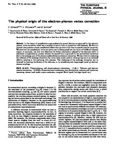
Fig. 1. (a) Electron self-energy. The open circle represents the set Γ of all irreducible vertex diagrams. (b) Expansion of Γ . The first diagram represents the bare electron-phonon interaction g(q) while the second one is the first vertex correction g(q)P (k + q, k) which in the adiabatic limit gives a negligible contribution to Σ.
due to its perturbative nature, the nonadiabatic theory does not describe polaron (bi-polaron) formation1 . In a recent series of papers, we have adopted the perturbative approach by retaining the first corrections beyond Migdal’s limit for both the superconductive transition and the normal state [12,13]. We have shown that the first vertex corrections already lead to a rich variety of behaviors ranging from the amplification of Tc [12] to the isotope dependence of the effective charge carrier mass [14]. The latter finding actually provides a possible interpretation of the experimental results given in reference [15]. Other interesting effects are given by the behavior of the pressure coefficient of Tc [16] and the tunneling current in the superconducting state [5]. Recently, we have shown that the presence of isotropic disorder leads to a suppression of the critical temperature Tc for nonadiabatic superconductors with s-wave symmetry of the gap [17]. The latter result provides a possible interpretation for the effects observed in K3 C60 [18] and in the electron doped cuprate Nd2−x Cex CuO4−δ [19], which are both s-wave superconductors. The variety of the effects cited above is a consequence of the non-trivial behavior of the first vertex corrections beyond Migdal’s limit. A typical vertex correction is given by the last diagram in Figure 1b where the solid and wiggled lines refer to electron and phonon propagators, respectively (see also the following section). There is a 1
It is here important to stress that polaron formation is a non-perturbative outcome of the electron-phonon system. For the one-electron case of the Holstein model see for example references [10, 11]
rather vast literature on the behavior of this and other nonadiabatic diagrams [20–28]. However, the main feature of the vertex function is that it changes sign according to the sizes of the momentum transfer q and the exchanged Matsubara frequency ω. In particular, the vertex is positive for vF |q|/ω � 1 and negative for vF |q|/ω � 1, where vF is the Fermi velocity [12,13]. Hence, depending on the typical values of vF |q| and ω, the total electron-phonon scattering amplitude can be larger or smaller than the corresponding quantity without vertex correction. It is basically from this property that the critical temperature Tc can be enhanced or lowered depending whether vF |q|/ω0 � 1 or vF |q|/ω0 � 1, respectively [12,13]. The results obtained by considering van Hove singularity effects [29] and by employing numerical calculations with tight-binding electron dispersions [30] have confirmed that such a behavior of the vertex function is rather robust. This situation suggests that the vertex diagram is more than just a mathematical function, leading to the possibility that its behavior can actually be interpreted in terms of physical processes. In particular, it would be interesting to understand which kind of physical processes of the electron-phonon system makes the vertex positive for vF |q|/ω < 1 and negative for vF |q|/ω > 1. In this paper we try to clarify this point by investigating the physics governing the behavior of the vertex function. Concerning the theory of nonadiabatic superconductivity, the interpretation of the nonadiabatic corrections in terms of physical processes is important for several reasons. First, it permits to identify the characteristics of the materials which can lead to an enhancement of the critical temperature. Moreover, the physical understanding of the nonadiabatic effects can in principle overcome the limitations of our perturbative theory by showing the way to construct a phenomenological theory no longer bound to the diagrammatic structure. Finally, our analysis permits also to reconsider the electron-phonon coupled system and Migdal’s theorem itself from a point of view different from the usual ones, certainly contributing to the understanding of the problem. In the following part of this paper we first summarize the behavior of the vertex function for different values of the ratio ω0 /EF and of the electron-density n. In Section 3 we focus on the one-electron case and the anti-adiabatic limit ω0 → ∞. For these two cases the interpretation in terms of physical mechanisms turns out to be particularly straightforward. The last section is devoted to a general discussion and to the conclusions.
2 Behavior of the vertex function In this section we consider the electron-phonon vertex correction and its behavior as a function of the adiabatic parameter ω0 /EF and the electron density n. In the present analysis, we neglect the Coulomb interaction between electrons. Let us consider an Hamiltonian describing electrons with dispersion �k interacting with phonons via a momentum dependent electron-phonon
C. Grimaldi et al.: The physical origin of the electron-phonon vertex correction
matrix element γq : � � H= �k c†kσ ckσ + ω0 b†q bq +
�
k,q,σ
0.6
Q=0.0 0.4
Q=0.2
q
� � γq c†kσ ck−qσ bq + b†−q .
0.2
(1)
Here, ω0 is the phonon frequency, assumed to be dispersionless for simplicity, and c†kσ (ckσ ) is the creation (annihilation) operator for an electron with wave number vector k and spin σ. b†q (bq ) is the creation (annihilation) operator for phonons with momentum q. The thermal Green’s function for the electron G(k) satisfies the usual Dyson equation: G−1 (k) = G−1 0 (k) − Σ(k),
(2)
where we have used the four-momentum representation k ≡ (k, iωk ) ωk = (2nk + 1)πT is the fermionic Matsubara frequency and T is the temperature. In equation (2), G−1 0 (k) = iωk − �k and Σ(k) is the electron self-energy due to the electron-phonon coupling: � Σ(k) = gq2 Γ (k + q, k)D(q)G(k + q), (3) q
where we have used the short notation: � �� ≡ −(T /N ) . q
ωq
q
In the above equation, gq2 = 2γq2 /ω0 and D−1 (q) = D0−1 (iωq ) − Π(q) is the phonon propagator, where Π(q) is the corresponding self-energy and D0 (iωq ) =
ω02 (iωq )2 − ω02
(4)
is the free propagator for phonons with Matsubara frequencies ωq = 2nq πT . In the following, the variable q ≡ (q, iωq ) will always refer to phonons. In terms of Feynmann diagrams the self-energy (3) is shown in Figure 1a, where the solid and wiggled lines are electronic and phononic propagators, respectively. In Figure 1a the open circle is the proper vertex function Γ (k + q, k), which is given by all diagrams which cannot be separated into two different contributions by cutting a single electron or phonon propagator line. In Figure 1b, we show the expansion of the vertex function up to the first correction: Γ (k + q, k) = 1 + P (k + q, k), where the vertex correction P (k + q, k) is given by the following expression: � 2 � � � P (k + q, k) = gk−k (5) � D(k − k )G(k + q)G(k ). k�
The aim of the present paper is to provide a physical interpretation of the above vertex correction. In this way, we should be able also to interpret in terms of physical processes its complex behavior already pointed out in references [7,12,13,29] and that we remind here briefly. First,
Q=0.4 Q=0.6
P(k+q,k)
k,σ
249
0.0
Q=0.8
−0.2 −0.4
ω0/EF=1.0
−0.6 −0.8 0.0
1.0
2.0
3.0
ω/ω0 Fig. 2. Vertex function P (k + q, k) as a function of the exchanged frequency and for different values of the dimensionless momentum transfer Q = q/(2kF ). The calculations have been performed by using a flat density of states and a structureless electron-phonon coupling.
Migdal’s theorem states that the order of magnitude of the vertex correction (5) is P (k + q, k) ∼ λω0 /(vF |q|), where λ � �gq2 �/EF is the electron-phonon coupling and vF is the Fermi velocity. Since in conventional metals λ < 1 and the momentum transfer |q| is of order of the Debye momentum qD , ω0 /(vF qD ) � ω0 /EF � 1, where we have set qD � kF . The vertex correction P (k + q, k) can be therefore safely neglected and Γ � 1. This simple argument needs to be refined for systems showing a strong energy dependence of the electronic density of states (see for example Refs. [25,29]). However, whatever the details of the band structure are, when ω0 is of the same order of the electron bandwidth or when |q| � kF , the vertex correction is no longer negligible. This situation can be outlined by approximating the electron and phonon propagators, G and D, with their corresponding free forms G0 and D0 . In this way, the sum over Matsubara frequencies in equation (5) can be performed exactly and the vertex correction reduces to the following form: P (k + q, k) =
2 gk−k ω0 � � 2 � �k� − �k� +q + iωq k
×
�
f (�k� ) + n(−ω0 ) f (�k� ) + n(ω0 ) − �k� + ω0 − iωk �k� − ω0 − iωk
� f (�k� +q ) + n(−ω0 ) f (�k� +q ) + n(ω0 ) − + · �k� +q + ω0 − i(ωk + ωq ) �k� +q − ω0 − i(ωk + ωq ) (6) In the above equation, f and n are the fermionic and bosonic distribution functions, respectively. By employing various approximations like for example the ones used in references [12,13] (constant electron density of states, structureless electron-phonon coupling and small momentum transfer) it is possible to perform
250
The European Physical Journal B
q k’ k’+q
Fig. 3. Representation of the particle-hole phase space. The shaded area is the Fermi see, the open circle an hole and the filled circle an electron. For zero exchanged frequencies, particle-hole excitations can be obtained by connecting the hole with the electron by the momentum transfer q such that q · k� = 0.
the frequency-momentum dependence is very sensitive of the band-filling has already been demonstrated in reference [30] where it has been shown that, by moving toward the low density limit, the momentum dependence is weakened and the vertex becomes mainly positive (see Fig. 2 of Ref. [30]), in agreement with previous results obtained in the infinite coordination lattice limit [32]. Summarizing the above discussion, P (k + q, k) has a strong dependence on the exchanged frequency and momentum, and in particular is non-analytic in ωq = 0, q = 0, only when the electron density is finite.Such a behavior is typical of several response functions, and it results from the presence of particle-hole excitations. These kinds of excitations are also present in the vertex function (6) and they can be explicitly singled out by rearranging equation (6) in the following way: P (k + q, k) = Ppol (k + q, k) + Pex (k + q, k),
analytically the remaining summation in equation (6). The result is shown in Figure 2, where we plot the vertex correction P (k + q, k) at half filling as a function of the exchanged frequency ωq and for different values of the dimensionless momentum transfer Q = |q|/(2kF ). For simplicity, the external electron frequency ωk has been set equal to zero. In the figure we notice that P (k + q, k) can assume positive and negative values depending on the ratio vF |q|/ωq : for vF |q|/ωq < 1 the vertex is positive while for vF |q|/ωq > 1 the vertex becomes negative. This complex behavior is found also for more realistic band models [30] and it is also reflected in the different values the vertex assumes in the dynamic and static limits. In fact, within the same approximation scheme used in the calculations reported in Figure 2, the static limit Ps = limq→0 limωq →0 P (k + q, k) is negative: Ps = −ω0 /(ω0 + EF ), while the dynamic one Pd = limωq →0 limq→0 P (k + q, k) is instead positive: Pd = EF /(ω0 + EF ) [7,12,13]. The vertex correction is therefore non-analytic in ωq = 0, q = 0. This situation holds true also when we consider strongly energy dependence in the density of states. In fact, in the presence of a Van Hove singularity, the expressions for Pd and Ps differ from the above simple results but the non-analyticity in ωq = 0, q = 0 remains [29]. However, this non-analyticity is removed when we consider the case of only one electron coupled to the lattice. In this situation the electron distribution functions in (6) are strictly zero [31] and the vertex correction reduces to: P (k + q, k) =
ω0 � 2 g � 2 � k−k
+
�
n(ω0 ) (�k� − ω0 − iωk )(�k� +q − ω0 − iωk − iωq )
(�
k�
�
1 + n(ω0 ) , + ω0 − iωk )(�k� +q + ω0 − iωk − iωq )
where Ppol (k + q, k) =
ω0 � 2 g � 2 � k−k k
×
−
�
(�k�
(�k�
f (�k� ) + n(ω0 ) − ω0 − iωk )[�k� +q − ω0 − i(ωk + ωq )]
� 1 + n(ω0 ) − f (�k� ) , + ω0 − iωk )[�k� +q + ω0 − i(ωk + ωq )]
(9)
and Pex (k + q, k) = −
�
2 gk−k �
k�
×
ω02 (iωk + iωq − �k� +q )2 − ω02
f (�k� +q ) − f (�k� ) · �k� +q − �k� − iωq
(10)
The vertex function Ppol , equation (9), has equal dynamic and static limits and, in the one electron case, it reduces to equation (7). The second function, Pex , has instead a non-zero static limit and vanishes in the dynamic limit. Moreover, contrary to Ppol , Pex vanishes in the one electron limit. It is therefore Pex that is responsible for the different values of the dynamic and static limits of the vertex function (6) when the electron density is finite. As it is clear from the expression in equation (10), the behavior of Pex is governed by particle-hole excitations since the factor f (�k� +q ) − f (�k� ) f (�k� +q )[1 − f (�k� )] = �k� +q − �k� − iωq �k� +q − �k� − iωq
k
×
(8)
+ (7)
and it is straightforward to realize that the dynamic and static limits of equation (7) are in fact equal. That
f (�k� )[1 − f (�k� +q )] , �k� − �k� +q + iωq
(11)
describes particle-hole pairs creation. The reason of having different values of the static and dynamic limits is contained just in equation (11). In fact, the particle-hole excitation processes depend strongly on the available phase
C. Grimaldi et al.: The physical origin of the electron-phonon vertex correction
space as it is shown in Figure 3 where we show schematically the process given by the last term of equation (11) for an isotropic Fermi sphere. For zero exchanged frequency, ωq = 0, particle-hole excitations are present when �k� +q = �k� , and this condition is obtained by placing the hole and the electron close to the Fermi surface. On the other hand, when the exchanged frequency is nonzero, the particle-hole excitations vanishes linearly with the momentum transfer q when q → 0. From the above discussion, we have seen that the two contributions Ppol and Pex to the vertex function P have different behaviors. In the following, we shall show that these different behaviors are due to the fact that Ppol and Pex actually have different physical interpretations, and the problem of finding the physical origin of the vertex P can be solved by looking separately at Ppol and Pex .
3 Limiting cases In this section we investigate the vertex function by considering its two components, Ppol and Pex , separately. This can be done by considering particular limiting cases. For example, in the limit of one electron in the system, the particle-hole contributions vanish so that Pex = 0 and the vertex function coincides with Ppol in the form of equation (7). On the other hand, as it is clear from equation (9), when we employ ω0 = ∞ limit (non-retarded phonon propagator) for a finite electron density, the polarization part Ppol vanishes and the vertex is determined entirely by limω0 →∞ Pex . The physical interpretation of the one electron and ω0 = ∞ limits becomes straightforward if we introduce an external potential Uext which couples to the electron density. In fact, when the coupling to the lattice is absent, this potential modifies the electron distribution in a way which depends on the explicit form of Uext . However, when the electrons interact with the phonons, the response of the electrons to the external potential changes because of the electron-phonon coupling. This situation can be described in terms of an effective potential Ueff . Actually, the vertex function is part of the effective potential, so that we can interpret the vertex correction in terms of the physically more intuitive Ueff . 3.1 One-electron case: Ppol First, we consider the case of only one electron in the system. In this situation, the particle-hole contributions of the vertex function vanish and the second term of equation (8), Pex , is zero. Therefore the vertex is given by the one electron limit of Ppol , equation (9), which at zero temperature reduces to: Ppol (k + q, k) = ω0 � 2
k�
As already pointed out before, the dynamic and static limits of Ppol coincide and, by using a constant density of states N (0) and a structureless electron-phonon interaction g0 (see Refs. [12,13]), the q = 0, ωq = 0 limit of (12) becomes: lim
ωq →0,q→0
(�k� + ω0 − iωk )(�k� +q + ω0 − iωk − iωq )
·
(12)
Ppol (k + q, k) = λ
E/2 , ω0 + E
(13)
where we have neglected the external electron frequency ωk . In the above equation, E is the electronic bandwidth and λ = g02 N (0) is the electron-phonon coupling constant. Our aim is to find the physical origin of equation (12) and to explain the reason why the limit in equation (13) is positive and, consequently, why the total effective nonadiabatic coupling is enhanced. To this end, we approach the problem by reasoning in terms of the electron response to an external potential Uext 2 . Let us for the moment neglect the electron-phonon interaction. For simplicity, we assume also that, in the absence of the external perturbation Uext , the electron wavefunction for the state k and energy �k is well √ described by a simple plane-wave ψk0 (r) = exp(ik · r)/ V , where V is the volume. A nonzero external perturbation Uext modifies the electronic wavefunction which, to the first order of the timeindependent perturbation theory, is given by: ψk (r) = ψk0 (r) +
� Uext (q) 0 ψk+q (r). � − � k k+q q
(14)
0 where Uext (q) = �ψk+q |Uext (r)|ψk0 �. If we consider Uext (r) to be given by a potential well of the form: � −U0 r ≤ R Uext (r) = (15) 0 r>R
then the density of probability |ψk (r)|2 of finding an electron with k = 0 at position r is enhanced inside the potential well and lowered outside the region r ≤ R. This is shown in Figure 4 where we plot V |ψk (r)|2 for k = 0 by a dashed line. In the lower panel of the same figure we also plot the potential well Uext (r) of equation (15) (dashed line). Let us now study how the above picture is modified when the electron is weakly coupled to the lattice vibrations. Intuitively, we expect that the lattice is more polarized where the probability of finding the electron is larger, that is inside the potential well (for k small). The lattice polarization, in turns, provides an attractive potential which is added to the external one. We can consider this situation in a formal way by replacing the simple plane waves ψk0 (r) in equation (14) and in the definition of Uext (q) by wavefunctions modified by the coupling to 2
2 gk−k �
251
Since in the one-electron case the static and dynamic limits of the vertex function are equal, we can consider a static potential (ωq = 0) and no ambiguity is found in the q = 0 limit.
252
The European Physical Journal B
2
1.1
V|ψ| , V|φ|
1.2
2
1.3
reported in Figure 4, where in the lower panel we plot the Fourier transform of the effective potential (18) for k = 0 (solid line). Moreover, the enhanced potential leads to an enhanced probability of finding the electron in the vicinity of the potential well (solid line in the upper panel of Fig. 18). At this point it is straightforward to understand why the q → 0 limit of the vertex function for one electron is positive (see Eq. (13)). In fact, for k = 0, limq→0 Ppol = �Ppol (r)�, where �· · · � means the average over the volume of the system, and from equation (18):
1.0 0.9 1
Uext, Ueff
0 −1 −2
�Ppol (r)� =
−3 −4
0
1
2
3
4
r/R
Fig. 4. Upper panel: density of probability of one electron in the presence of an external potential (plotted in the lower panel). Solid (dashed) lines: case with (without) electronphonon interaction. The potentials are plotted in units of U0 and the densities of probability are properly normalized. In order to make clear the effect of the electron-phonon coupling we have used suitable values of the parameters entering in equations (17, 18).
the lattice vibrations [31]: � ω0 � gk−k� 0 0 φk (r) = ψk (r) + b† � ψ 0 � (r). 2 � �k − �k� − ω0 k −k k k (16) In this way, the new electron wavefunction in the presence of the external potential reduces to φk (r) = φ0k (r) +
� Ueff (k + q, k) φ0k+q (r), �(k) − �(k + q) q
(17)
where �(k) is the electron dispersion modified by the electron-phonon coupling and Ueff (k+q, k) is the effective external potential which results from the lattice polarization: Ueff (k + q, k) = �φ0k+q |Uext (r)|φ0k � = Uext (q) � � 2 gk−k ω0 � � × 1+ . 2 � (�k� − �k + ω0 )(�k� +q − �k+q + ω0 ) k (18) The second term in square brackets is just the electronphonon vertex correction (12) calculated for iωk = �k and iωk +iωq = �k+q , i.e., at the poles of the incoming and outcoming electron lines of the vertex diagram of Figure 1b. The vertex correction for the one-electron case is therefore part of the effective potential arising from the lattice polarization. From the above discussion, as long as the electron is in phase with the lattice displacement, the polarization should in general amplify the potential seen by the electron. This is confirmed by the numerical results
�Ueff (r)� − �Uext (r)� > 0. �Uext (r)�
(19)
Of course the treatment of the problem followed in this section does not consider the effect of the other electrons when the electron density n is finite. This effect is partially contained in the general expression of Ppol given by equation (7) which in fact can be interpreted along the same lines followed in this section by taking into account the fermionic statistics of the electrons. However, Ppol is basically a single electron process and it belongs to the class of processes for which the same electron can generate a phonon at a certain time t and then absorb it at a later time t� . Such kind of processes are consequence of the retarded phonon propagation and they in fact vanish in the limit ω0 → ∞ (see Eq. (9)). On the other hand, for many electrons systems, different kinds of processes are those for which the electrons interact by exchanging virtual phonons. These are many-electrons processes not contained in Ppol but given by Pex , which is in fact determined by particle-hole excitations. In the next section we provide an interpretation for the physical origin of Pex . As anticipated before, we will introduce an external potential and we will consider the resulting effective potential by employing the ω0 → ∞ limit for which Ppol vanishes and the interpretation of Pex is particularly simple. 3.2 Anti-adiabatic limit: Pex Let us consider the electron-phonon coupled system in the limit ω0 → ∞. In order to have non-trivial results, we perform this limit in such a way that the quantity gq2 = 2γq2 /ω0 remains finite. From equation (9), limω0 →∞ Ppol = 0 and the vertex function reduces to: lim P (k + q, k) = lim Pex (k + q, k)
ω0 →∞
ω0 →∞
=
�
2 gk−k �
k�
f (�k� ) − f (�k� +q ) · (20) �k� − �k� +q + iωq
As we have seen before, this term has different dynamic and static limits. In particular, we have: lim
Pex (k + q, k) = 0,
lim
Pex (k + q, k) =
ωq →0,q→0
q→0,ωq →0
� k�
(21) 2 gk−k �
df (�k� ) � −λ, d�k� (22)
C. Grimaldi et al.: The physical origin of the electron-phonon vertex correction
where the last equality holds true at low temperatures and λ is the electron-phonon coupling constant. Although we can interpret the zero value of the dynamic limit (21) as due to the vanishing contribution of the hole-particle excitation contribution (see Eq. (11)), the reason why the static limit (22) is negative remains unclear. In this section we try to clarify this point by considering the problem of the electron response to an external potential Uext which couples to the electron density. The anti-adiabatic limit ω0 → ∞ transforms the electron-phonon interaction into an effective non-retarded electron-electron interaction. The Hamiltonian can be obtained by integrating out the phononic degrees of freedom [33] and then performing the ω0 → ∞ limit. The result is: H=
�
�k c†kσ ckσ +
� q
k,σ
1� 2 Uext (q)n(q)− g n(q)n(−q), 2 q q
(23)
where n(q) is the electron density operator: � † n(q) = ck+qσ ckσ .
(24)
kσ
Note that for the Holstein model gq = g0 , so that its anti-adiabatic limit is equivalent to the attractive Hubbard Hamiltonian with U = −g02 . Now, let us consider the response of the system to the external potential Uext . Since the electrons are interacting through gq2 , the response depends in general on the whole electron configuration. For our purposes, we shall deal with this problem by performing the Hartree-Fock approximation in the fouroperator term in equation (23). This approach is equivalent to consider antisymmetrized states of N independent one-electron wavefunctions and leads to the random phase approximation with exchange corrections for the effective potential seen by the electrons. When we apply the Hartree-Fock approximation, the interaction term in equation (23) becomes: � 1� 2 gq n(q)n(−q) → + gq2 �n(−q)�n(q) 2 q q � � − gq2 �c†k+qσ ck� σ �c†k� −qσ ckσ ,
+
�
(26)
where VHF is the Hartee-Fock potential in the presence of the external perturbation: � † 2 VHF (k + q, k) = −gq2 �n(−q)� + gk−k � �c � ck� +qσ �. kσ k�
(27)
+
δ�c†k� σ ck� +qσ �
(28) (29)
q kσ
0 where HHF is the Hamiltonian in the Hartree-Fock approximation for Uext = 0 and
Ueff (k + q, k) = Uext (q) + δVHF (k + q, k).
(31)
The above expression is a self-consistent equation because δVHF depends implicitly on Ueff . We can repeat the calculations by assuming a time-dependent external potential. In this case, by employing the linear response theory applied to the Hamiltonian (30), the self-consistent equation for Ueff is given by: Ueff (k + q, k, iωq ) = Uext (q, iωq )
+
k qσ
=
�c†k� σ ck� +qσ �0
where the first and the last terms in the right hand sides are the expectation values in the absence and in the presence of the external potential, respectively. From equa0 tions (27–29), VHF can be rewritten as VHF + δVHF and the Hamiltonian (26) becomes: � 0 H = HHF + Ueff (k + q, k)c†k+qσ ckσ , (30)
(25)
q
VHF (k + q, k)c†k+qσ ckσ ,
�n(−q)� = �n(−q)�0 + δ�n(−q)� �c†k� σ ck� +qσ �
� f (�k� ) − f (�k� +q ) k�
and, after a manipulation of the momenta indexes, the Hamiltonian (23) can be rewritten as follows: � � H= �k c†kσ ckσ + Uext (q)n(q) k,σ
The first term in the right hand side is the Hartree contribution which results from the potential generated by the electrons regardless the specific electronic configuration. The last term of equation (27) is instead the Fock contribution which treats the electrons as being dressed by their exchange holes. Below we show that the vertex function Pex originates from the Fock contribution of equation (27), i.e., from the exchange term of the phonon mediated electron-electron interaction. The effective potential given by the redistribution of the electrons is readily obtained by the linear response theory. In fact, for small values of Uext , the expectation values appearing in equation (27) can be rewritten as:
− 2gq2
q k k� σ
253
� k�
2 gk−k �
�k� − �k� +q + iωq
Ueff (k� + q, k� , iωq )
f (�k� ) − f (�k� +q ) Ueff (k� + q, k� , iωq ), �k� − �k� +q + iωq
(32)
where ωq is the Matsubara frequency provided by the time-dependence of the external potential and �k is now the electron dispersion in the Hartree-Fock approximation. Equation (32) is just the random phase approximation with exchange corrections applied to the electron-phonon coupled system in the anti-adiabatic limit ω0 → ∞. The second term of equation (32) represents the electron response to Uext governed by the Hartree potential while the last term is the correction due to the exchange potential. To the first order in Uext , the last term of equation (32) can be rewritten as Pex Uext where Pex is the vertex correction in the antiadiabatic limit (20). Therefore Pex is
254
The European Physical Journal B
=
+
+
Fig. 5. Diagrammatic representation of the self-consistent equation (32). The dashed circles represent the effective potential Ueff . The second diagram comes from the Hartree interaction while the last one from the Fock term. The wiggled lines represent the phonon mediated electron-electron interaction in the antiadiabatic limit.
just the Fock contribution to the electronic response to the external potential when ω0 → ∞. We show in Figure 5 the diagrammatic representation of the self-consistent equation (32). The Hartree term is represented by the set of bubble diagrams while the Fock contribution is given by the ladder contribution which, to the first order in Uext , is the vertex diagram. At this point we can explain the behavior of the vertex function in the antiadiabatic limit already outlined in equations (21, 22). In fact, the negative static limit of equation (22) can be understood by the following reasoning. If we consider a static potential, then we must set ωq = 0 in equation (32). For simplicity let us also consider an attractive potential like for example the one in equation (15), i.e., the potential well model. If we neglect the Fock contribution, the electrons will tend to form a cloud around the potential well and an added electron will experience an effective potential given by the bare potential well Uext plus the electron cloud. The resulting effective potential is given by the first two terms of the right hand side of equation (32). Since the phonon mediated el-el interaction is attractive, such an effective potential is stronger than the bare one. However, when we consider the effect of Pauli principle, the electron becomes dressed by the exchange hole which repels the other electrons. Therefore the net effect of the Pauli principle is to weaken the electron-electron attraction and this weakening is reflected in the negative sign of the exchange term. In conclusion, in the anti-adiabatic limit, the negative sign of the vertex function for ωq = 0, equation (22), is exclusively due to the exchange effect which weakens the phonon mediated electron-electron interaction. This picture is still valid when we take into account the retardation of the phonon-mediated electron-electron
interaction (ω0 < ∞). In fact the last term of equation (9) can be interpreted as the Fock-like contribution for a retarded potential.
4 Discussion and conclusions From the above analysis, we have seen that the vertex function results from electron-phonon processes of different origins. In fact, we have shown that the behavior of the vertex P is due to the competition between two different contributions: Ppol and Pex . The first one is the result of the lattice polarization as induced by the electron motion. At low frequencies, this term leads to a positive contribution to the electron-phonon interaction and tends to enhance the coupling. Moreover, Ppol is basically a single electron process. The second term, Pex , is instead due to the exchange effect of the phonon mediated electron-electron interaction. Due to its nature, Pex tends to reduce the electron-phonon effective coupling. Moreover, since the exchange term gives rise to particle-hole excitations, Pex is sensitive to the momentum transfer q and the exchanged frequency ωq of the electron-phonon scattering process and it gives rise to the different values of the dynamic and static limits of the vertex function. In particular, for vF |q| � ωq the vertex function is mainly a lattice polarization process while for vF |q| � ωq the polarization is reduced by the exchange hole. Given the results presented in this work, it is possible to identify situations in which the vertex correction can give rise to an enhancement of the effective electronphonon coupling. In fact, an enhancement can be automatically obtained if the exchange effects become less important. This can be achieved, for example, when the charge carrier density is low, so that the average distance between electrons can exceed the size of the exchange hole leading to a negligible Pex . In this way we can understand the results reported in references [30,32] where it is shown that, by reducing the charge carrier density, the vertex correction enhances the effective coupling. A more interesting situation in favour of an enhancement of the vertex corrected electron-phonon coupling is obtained by considering only small q scattering in the electron-phonon interaction. In fact, for a small enough momentum transfer, say vF |q| � ω0 , the particle-hole contributions (11) have little weight and the negative exchange term Pex becomes negligible. This result therefore clarifies on physical grounds why the effective nonadiabatic electron-phonon interaction and so the superconducting critical temperature Tc is enhanced by the vertex corrections when the electron-phonon interaction is only via small momentum transfer [12,13]. At this point, it is useful to briefly summarize the role played by strong electronic correlations on the size of the electron-phonon momentum transfer. As it is well know, in ordinary superconductors the phase space available for large momentum transfer phonons is much larger than for small momentum transfer phonons because the correlation is weak and the screening important. In this situation therefore the main contribution comes from the static
C. Grimaldi et al.: The physical origin of the electron-phonon vertex correction
limit Ps of the vertex corrections. For ω0 /EF � 1 Ps is negligible and Migdal’s theorem holds true. However, in materials where the electronic correlation is strong, the situation may differ substantially as reported by several authors in recent years [34–39]. The physical picture common to the different theoretical approaches is that, in a strongly correlated system, the charge carriers are surrounded by giant correlation holes that may extend over many lattice units [39]. For example, in the U → ∞ limit of the Hubbard model, the correlation hole has an extension of roughly a/δ, where a is the lattice constant and δ is the hole concentration [39]. In this case, the system can respond only to charge fluctuations of characteristic length larger than a/δ. In this way, the maximum electronphonon momentum transfer is of order δ/a, which can be much less than the unity for low hole concentrations. Such a small momentum transfer can suppress the exchange contribution (10) and single out only the positive polarization part of the vertex function (Eq. (9)). Finally, it should be remarked that an electron-phonon interaction peaked at small momentum transfer is also a natural consequence of weak screening effects when the charge carrier density is small [40]. We would like to thank A. Amici, E. Cappelluti, S. Ciuchi, A. Perali and S. Str¨ assler for useful discussions. C. G. acknowledges the support of a INFM PRA project (PRA-HTCS).
References 1. A.B. Migdal, Zh. Eksp. Teor. Fiz. 34, 1438 (1958) [Sov. Phys. JETP 34, 996 (1958)]. 2. Y.J. Uemura, L.P. Le, G.M. Luke, B.J. Sternlieb, W.D. Wu, J.H. Brewen, T.M. Riseman, C.L. Seaman, M.B. Maple, M. Ishitawa, D.G. Hinks, J.D. Jorgensen, G. Saito, H. Yamochi, Phys. Rev. Lett. 66, 2665 (1991). 3. J.R. Schrieffer, J. Low Temp. Phys. 99, 377 (1995). 4. O. Gunnarsson, Rev. Mod. Phys. 69, 575 (1997). 5. G.A. Ummarino, R.S. Gonnelli, Phys. Rev. B 56, R14279 (1997). 6. L. Pietronero, Europhys. Lett. 17, 365 (1992). 7. L. Pietronero, S. Str¨ assler, Europhys. Lett. 18, 627 (1992). 8. A.S. Alexandrov, Physica C 158, 337 (1989). 9. B.K. Chakraverty, J. Ranninger, D. Feinberg, Phys. Rev. Lett. 81, 433 (1998). 10. S. Ciuchi, F. de Pasquale, S. Fratini, D. Feinberg, Phys. Rev. B 56, 4494 (1997). 11. M. Capone, S. Ciuchi, C. Grimaldi, Europhys. Lett. 42,
255
523 (1998). 12. C. Grimaldi, L. Pietronero, S. Str¨ assler, Phys. Rev. Lett. 75, 1158 (1995). 13. L. Pietronero, S. Str¨ assler, C. Grimaldi, Phys. Rev. B 52, 10516 (1995); C. Grimaldi, L. Pietronero, S. Str¨ assler, Phys. Rev. B 52, 10530 (1995). 14. C. Grimaldi, E. Cappelluti, L. Pietronero, Europhys. Lett. 42, 667 (1998). 15. G.M. Zhao, M.B. Hunt, H. Keller, K.A. M¨ uller, Nature 385, 236 (1997). 16. S. Sarkar, Phys. Rev. B 57, 11661 (1998). 17. M. Scattoni, C. Grimaldi, L. Pietronero, cond-mat/9812192 (1998). 18. S.K. Watson, K. Allen, D.W. Denlinger, F. Hellmann, Phys. Rev. B 55, 3866 (1997). 19. S.I. Woods, A.S. Katz, M.C. de Andrade, J. Herrmann, M.B. Maple, R.C. Dynes, Phys. Rev. B 58, 8800 (1998). 20. T. Holstein, Ann. Phys. 29, 410 (1964). 21. M. Grabowsky, L.J. Sham, Phys. Rev. B 29, 6132 (1984). 22. J. Cai, L. Lei, L.M. Xie, Phys. Rev. B 39, 11618 (1989). 23. V.N. Kostur, B. Mitrovi´c, Phys. Rev. B 48, 16388 (1993); 50, 12774 (1994). 24. Y. Takada, J. Phys. Chem. Solids 54, 1779 (1993); Y. Takada, T. Higuchi, Phys. Rev. B 52, 12720 (1995). 25. H.R. Krishnamurthy, D.M. Newns, P.C. Pattnaik, C.C. Tsuei, C.C. Chi, Phys. Rev. B 49, 3520 (1994). 26. O. Gunnarsson, V. Meden, K. Sch¨ onhammer, Phys. Rev. B 50, 10462 (1994). 27. J.K. Freericks, E.J. Nicol, A.Y. Liu, A.A. Quong, Phys. Rev. B 55, 11651 (1997). 28. M. Mierzejewski, J. Zieli´ nski, P. Entel, Phys. Rev. B 57, 590 (1998). 29. E. Cappelluti, L. Pietronero, Phys. Rev. B 53, 932 (1996); Europhys. Lett. 36, 619 (1996). 30. A. Perali, C. Grimaldi, L. Pietronero, Phys. Rev. B 58, 5736 (1998). 31. G.D. Mahan, Many-Particle Physics (Plenum Press, N.Y. and London, 1990). 32. J.K. Freericks, Phys. Rev. B 50, 403 (1994). 33. R. Brendle, R. Zeyher, Z. Phys. B 69, 263 (1987). 34. K.J. von Szczepanski, K.W. Becker, Z. Phys. B 89, 327 (1992). 35. H. Kim, Z. Tesanovic, Phys. Rev. Lett. 71, 4218 (1993). 36. M. Grilli, C. Castellani, Phys. Rev. B 50, 16880 (1994). 37. J.D. Lee, Kicheon Kang, B.I. Min, Phys. Rev. B 51, 3850 (1995). 38. R. Zeyher, M. K´ ulic, Phys. Rev. B 53, 2850 (1996). 39. O.V. Danylenko, O.V. Dolgov, M.L. K´ ulic, V. Oudovenko, Eur. Phys. J. B 9, 201 (1999). 40. M. Weger, M. Peter, L.P. Pitaevskii, Z. Phys. B 101, 573 (1996).