The Longterm Effects of UI Extensions on Employment Johannes F. Schmieder, Till von Wachter and Stefan Bender∗ January 22, 2012 The effect of extending the duration of unemployment insurance (UI) benefits on nonemployment duration is a hotly debated question. The vast majority of the literature (e.g., Katz and Meyer 1990, Schmieder, von Wachter, and Bender 2012) [henceforth SVB]) analyzes the effect of extensions in UI durations or increases in UI benefits on the initial nonemployment spell. This may lead to an understatement of the cost of UI extensions, if such extensions increase the incidence of nonemployment beyond the initial spell, as would be predicted by models of stigma, skill depreciation, or supply-side hysteresis (e.g., Blanchard and Diamond 1994, Lemieux and MacLeod 2000). On the other hand, these estimates may overstate employment effects if longer initial spells tend to reduce future incidence of nonemployment. This might arise because of an increase in individual labor supply, for example due to lower income. In addition, with a finite lifetime (or a finite follow-up period) the nonemployment effect can also decline mechanically. This can arise since at a given, say, monthly probability of being unemployed, individuals with longer initial spells accumulate less time in nonemployment due to a shorter remaining lifetime. Despite these alternative hypotheses, little is known about the longer-term effect of UI extensions on employment. In this paper, we make two contributions. First, we use a regression discontinuity design to analyze the long-term effects of extensions in UI durations. These estimates differ from standard estimates that they incorporate differences in UI benefit receipt and employment due to recurrent unemployment spells. Second, we extend the welfare formula of UI extensions from SVB to incorporate recurrent nonemployment spells.

1

Welfare Formula with Long-Term Effects of UI Extensions

In this section we extend the welfare effect of UI extensions derived in SVB to incorporate long-term effects of UI benefit durations on nonemployment. The key difference is that instead of modeling the individual job seeker’s choice of reservation wages, we generalize the model to a choice of reservation match-quality, and hence of expected job duration. ∗ Schmieder: Boston University, 270 Bay State Rd, 02215 Boston, MA, [email protected]. von Wachter: Columbia University, 420 W 118th St., New York, NY 10025, [email protected]. Bender: Institute for Employment Research (IAB), Regensburger Str. 104, 90478 Nuremberg, Germany, [email protected]. We would like to thank our discussant Bruce Meyer for many useful comments. Johannes Schmieder gratefully acknowledges funding from the 2011 Scholars Program of the Department of Labor. All errors are our own.

1

Our model is closely based on SVB (2012), which in turn draws on Chetty (2008). As in SVB, unemployed job seekers choose how intensely to search for a job, while receiving a fixed UI benefit at a fixed duration. In contrast to SVB and related papers, instead of receiving a job at a given wage and accepting based on a reservation wage strategy, we assume workers receive a job at a fixed wage, but at a variable probability of layoff that is drawn from a stationary stochastic job offer distribution. In this case, we show that under common assumptions job search behavior is described by a reservation layoff probability. Jobs with layoff probabilities above the reservation values are accepted. As in the basic model, workers face a liquidity constraint, and the policy maker chooses the duration of UI benefits at a constant level. Our decision to model job search as a choice of a reservation layoff probability rather than a reservation wage can be interpreted in several ways. On the one hand, wages may vary little within a job class defined by occupation, industry, and previous job seniority; hence, individuals have less of a choice over wages but look for jobs that provide a good fit and hence last longer. This is not a bad assumption in Germany, were wages in many jobs are traditionally set by collective bargaining. On the other hand, one can interpret our model more generally as a choice of reservation match quality, which may be related to multiple possible job attributes, such as job duration, wages, commuting times, or work environment. In this context, our approach provides a convenient short cut relative to explicitly considering job search over multiple job attributes. It is also sensible because job duration is frequently used as an index of job quality, given that wages can incorporate compensating differentials and hence do not fully represent a job’s attractiveness. After some algebra, which is summarized in our companion Web Appendix, the effect on social welfare W0 of an extension of potential UI durations P can be expressed as

i dB h dW0 = b E0,T −1 u0 (cut,P ) − E0,T −1 v 0 (cet ) dP dP 1

−

dB B dD + dP 2 T − D dP

!

b E0,T −1 v 0 (cet )

where E0,T −1 u0 (cut,P ) and E0,T −1 v 0 (cet ) are the expected marginal utilities at benefit exhaustion and upon reemployment, respectively; T , B, and D represent total remaining life time, total benefit duration, and total nonemployment duration; dB/dP |1 is the average exhaustion rate, and dB/dP |2 is the effect of potential UI benefit duration on duration of UI benefit receipt prior to benefit exhaustion (such that the effect of a extension in UI duration on total benefit duration is dB/dP = dB/dP |1 +dB/dP |2 ); and dD/dP is the corresponding effect on total nonemployment duration. The formula has the same structure as that derived in SVB; i.e., the welfare gain of UI extensions depends on the exhaustion rate, and is proportional to the difference in marginal utility of a worker exhausting UI benefits relative to her utility at reemployment. The welfare cost is the increase in taxes due to UI extensions, which results from a rise in total payouts without corresponding welfare benefits and a decline in the number of individuals paying taxes. The key difference with respect to the formula in SVB is that here B and D represent total duration of UI benefits and nonemployment after the start of the initial spell. I.e., 2

10

15

20

25

30

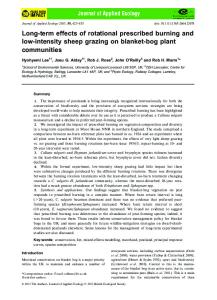
they depend both on the duration of the initial UI and nonemployment spell, as well as the incidence and duration of recurring UI and nonemployment spells. How this difference affects estimates of the effect of UI extensions is subject of our empirical analysis. A noteworthy feature of the welfare equation we derived here is that any effect of UI extensions on job durations or match quality other than what affects the incidence and duration of UI and nonemployment spells does not affect welfare directly. As noted by Chetty (2008), this results from an application of the envelope theorem. This welfare equation does not take into account potentially important channels through which UI extension can affect nonemployment and welfare, such as general equilibrium effects of UI extensions. Below, we will nevertheless use the welfare equation to calibrate the welfare effects of UI extensions Days per month nonemployed by Month with and without accounting for longer-term effects.

0

20

40

60

Month since UI claim 12 Months Potential UI Duration

18 Months Potential UI Duration Number P=12: 258413, Number P=18: 252683

Figure 1: Days nonemployed per month The difference between the lines is estimated using a regression discontinuity design. Vertical bars indicate statistical significance.

2

Regression Discontinuity Estimates of Dynamic Effects of UI Extensions

In this section, we present regression discontinuity (RD) estimates using the same research design as in SVB, with three differences. First, our main outcome variables are the total days receiving UI benefits and the total days in nonemployment in the first five years after the start of the initial UI spell, irrespective of whether the initial spell has ended or not. Hence, in contrast to previous estimates this captures nonemployment effects from recurring spells. Second, we replicate the RD estimate for UI and nonemployment duration in each month since the start of the initial spell, again irrespective of whether the initial spell has 3

ended. We use these estimates to construct dynamic figures capturing the long-term impact of UI extensions. Finally, we provide preliminary estimates decomposing the effect on the total nonemployment duration into a change in the incidence of nonemployment in any given month after the initial spell has ended and a mechanical effect arising from a shorter remaining time horizon over which individuals with higher potential UI durations can accumulate time spent in nonemployment. In Germany, after having worked at least 12 months to be covered, in the period from 1987 to 1999 unemployed workers were eligible to receive UI benefits at a fixed replacement rate for a fixed number of months (See SVB for details). The duration was a function of exact age at application for benefit receipt and the amount of labor force experience. Here, we focus on the discontinuity at age 42 for workers that worked at least three out of the last seven years without UI spell, for whom maximum duration of UI benefits rose from 12 to 18 months. We focus on the earliest cutoff point available to maximize our sample size and follow up duration. Table 1: The Effect of UI Benefit Extensions on Long-term Employment (1) (2) (3) (4) Sum of days Sum of days UI Benefit Nonemp. on UI benefits nonemployed Duration in Duration over 5 years over 5 years 1st Nonemp spell until 1st job D(Age≥42)

68.2 [1.28]** dy 11.4 dP [0.21]** Observations 489275 Mean of Dep. Var. 341.3 Coefficients from RD regressions. Local cutoff. Standard errors clustered on day

28.1 54.3 37.9 [4.07]** [1.10]** [4.27]** 4.68 9.15 6.32 [0.68]** [0.71]** [0.71]** 489275 489275 489275 892.9 237.9 626.1 linear regressions (different slopes) on each side of level (* P<.05, ** P<.01)).

We implement a straightforward regression-based RD analysis using a two-year bandwidth around the age cutoff and allowing for a differential linear impact of claiming age on each side of the age cutoff.1 We use administrative records from Germany covering the period from 1975 to 2004, which provide us with information on exact day of birth, basic demographic and job characteristics, as well as day-to-day UI and employment spells for the universe of employees covered by social security. We extract individuals age 40 to 43 that satisfy the labor force experience criterion who became unemployed between 1987 and 1999. Our main outcome measures are days receiving UI benefits and days in nonemployment at any time within five years after the start of the initial UI spell. Figure 1 displays the average number of days in nonemployment in each month after start of benefit receipt for the group of workers with 12 months and with 18 months UI duration. 1

In SVB, we discuss the possibility that workers might selectively apply for benefit durations before and after the age thresholds, and conclude that any impact of selection is likely to be small in our context. Similarly, we examined the sensitivity of our estimates to modelling choices.

4

The vertical bars represent RD estimates based on information on nonemployment duration in the respective month for workers above and below the 42 age cutoff. The structure of the estimates is analogous to that of a classic event study and differs from standard hazard functions, which only follows individuals until the exit from their first unemployment spell. The figure makes three points. First, nonemployment durations are higher for workers eligible for higher benefits even in the months before there is a difference in eligibility. Hence, workers appear to be forward looking in their labor supply choices. Second, there is a slightly larger difference in nonemployment 12 to 18 months after the start of the initial spell, when eligibility for benefits differs. Thus, an important part of the effect of UI extensions indeed works through an extension of the first spell, as captured by standard estimates. Finally, the figure shows that the differences in nonemployment last well beyond exhaustion at 18 months. Nonemployment is significantly higher for workers with higher initial UI duration up to five years after the start of the initial spell. Although the differences appear to have essentially faded after five years, they are economically significant at least up to three years after the initial start of unemployment. Table 2: Decomposing the Long-term Employment Effects of UI Extensions (1) (2) Prob of unemp Covariance bw after reemp D1 and pu pu Cov(D1 , pu ) D(Age≥42)

-0.0046 -2.32 [0.0016]** [0.86]** dy -0.00076 -0.39 dP [0.00027]** [0.14]** Observations 489275 489275 Mean of Dep. Var. 0.18 -49.4 Coefficients from RD regressions. Local linear regressions (different slopes) on each side of cutoff. Standard errors clustered on day level (* P<.05, ** P<.01)). Figure 1 represents the combined effect from the initial nonemployment spell and differences in the incidence and duration of additional nonemployment spells. To show directly how differentiating between the first and additional spells makes a difference, in Table 1 we present various estimates of the effect of UI extensions on the sum of days spent receiving UI benefits and in nonemployment over five years after the initial spell. When we incorporate all nonemployment spells into our estimate, an extension of six months in potential durations of UI benefits leads to an increase in 28.1 days in nonemployment (column 2). To gauge the difference that accounting for recurring UI and nonemployment spells does, in column 4 of Table 1 we show the corresponding result when we only measure the effect of UI extensions on the duration of the initial UI and nonemployment spell.2 At an increase of 37.9 days for a 2

Note that these estimates are expressed in days and show the effect for five years. The estimates in SVB, Table 2 are expressed in months and show the effect over three years. To express the results in terms of months, divide the estimates in Table 1 by 30.5.

5

six month UI extension, this estimate is substantially larger than the estimate in column 2. This implies that allowing for added nonemployment spells lowers the effect of UI extensions on days of nonemployment by about 10 days, a decline of about 26% relative to the standard estimate. Note that in contrast to this reduction, comparing column 1 and 3 of Table 1, the sum of days receiving UI benefits increases if we include additional spells. This is partly mechanical, since the German UI system allows individuals finding a job before exhaustion of UI benefits to carry over their remaining benefit duration to the next spell. This carry-over effect is larger for those with higher UI durations, a finding that we discuss further when considering welfare effects of UI extensions in Section III. To better understand the sources of the substantial decline in the effect of UI extensions on nonemployment durations due to incorporation of recurring spells we find, consider the following decomposition. Let D1 be the duration of the first nonemployment spell. Let pu be the probability of being nonemployed in a given month after the first nonemployment spell (this is a combination of the probability of being laid off again the the duration of the later unemployment spells). Then the total amount spent in nonemployment (until retirement or the 5 year horizon we consider here) of a given individual i can be expressed as Di = Di1 + (T − Di1 )piu . To obtain a marginal effect of UI extensions on D for the population, take expectations of this expression and differentiate both sides with respect to potential UI duration P . This yields an expression for the difference between the the effect of UI extensions on total nonemployment (D) and unemployment in the first spell (D1 ), dD1 dpu dCov (D1 , pu ) dD = (1 − pu ) + (T − D1 ) − dP dP dP dP The difference arises from three sources. First, at a given propensity to spent time in nonemployment pu , a rise in the duration of the first spell reduces the total time spent in nonemployment in the remaining period (call this the ’mechanical’ effect). Second, the propensity of nonemployment in any given month may change; as mentioned at the outset, the sign of this effect is ambiguous. Third, the covariance between the duration of the first spell and the propensity to become nonemployed in the population may either rise or fall. The fact that the results in Table 1 indicate that the difference is negative, the decomposition suggests that either the ’mechanical’ effects dominates the two other components, or that it is reinforced by a decline in the propensity to become unemployed (or a change in the covariance term). To learn more about the three sources of the difference between the standard and more inclusive estimates of the nonemployment effect of UI durations, we calculated the effect of UI extensions on the monthly propensity to become nonemployed (pu ) and its covariance with the duration of the initial spell. These results are shown in Table 2. The mean of pu is 0.18, and the covariance term is negative, suggesting that those individuals with longer initial spells have a lower subsequent probability to be nonemployed. The findings of the effect of UI extensions are quite striking. The propensity of being nonemployed declines for individuals with higher potential UI durations. To assess the magnitude of this effect, one has to multiply the change with (T − D1 ), the number of days outstanding in our five year window after the initial spell; the result suggests that the decline in pu contributes with a decline in 5.5 to the differences in the estimates in columns 2 and 3 in Table 1. I.e., a bit more than half of the decline in the nonemployment effect of UI extensions when we consider 6

all spells instead of just the first nonemployment spell is due to a decline in the propensity to be unemployed. The mechanical effect and a further decline in the covariance explain each about half of the remaining difference. The increase in the effect of UI extensions on UI benefit receipt and nonemployment durations may be due to a decline in the number of recurring nonemployment spells, as well as an reduction in the duration of such spells. A preliminary examination of this question suggested that the duration of future nonemployment spells is unaffected by UI extensions and that instead the incidence of new nonemployment spells declined slightly. Pursuing this decomposition is a useful goal for future work.

3

Discussion and Conclusion

We can use the modified welfare formula we derived to gauge the potential magnitude of positive and negative welfare changes due to the presence of persistent effects of UI extensions. As discussed in more detail in SVB, these results should be treated as illustrative and approximate rather than exact. To implement the welfare formula, we expressed it in terms of sufficient statistics (see our Web Appendix) and rescaled it by the marginal utility of the employed, so that welfare is expressed in monetary terms rather than utility. We require two additional inputs with respect to the results of the paper. First, we need an estimate of the ratio of income and substitution effects, which we take from Chetty (2008). Second, to implement the welfare formula we need to obtain estimates of dB/dP |1 and dB/dP |2 . However, we can use the fact that UI extensions do not increase the duration of additional spells to infer that the added time spent on UI due to a reduction in search (dB/dP |2 ) for the added spells is zero. Hence, all of the portion of dB/dP beyond the dB/dP |2 for the initial spell must be due to an increase in coverage and hence is welfare increasing. Using these assumptions and the estimates for the benefit and nonemployment effect of UI extensions in columns (1) and (2) of Table 1, we obtain that the welfare gain from UI extensions is 281 Euros per month of UI extension and per unemployed worker. If instead we use the estimates of the effect of UI extensions on the first spell in columns (3) and (4) of Table 1, the welfare gain is 192 Euro per month of UI extension. Given the increase in outlays in the former case, the difference in the welfare gain per Euro spent is smaller, 0.97 vs. 0.83, but still substantial in percentage terms. These numbers highlight that incorporating persistent effects of UI extensions on nonemployment durations can substantially change the welfare effect of UI extensions. The magnitude of the welfare gain depends crucially on how we decompose the total benefit increase into the exhaustion rate (dB/dP |1 ) and the component due to reduction in search effort (dB/dP |2 ). The reason is that dB/dP |1 is weighted by the ratio (here a value of 1.5) and dB/dP |2 enters the welfare equation as it is. On the other hand, the nonemployment effect, which has been the focus of a large literature, is multiplied by the unemployment rate (B/(T − D)) and hence changes in its value have rather small impact in the welfare formula we derived. While when only looking over a single spell we have that dD/dP is roughly proportional to dB/dP |2 and is thus a reasonable statistic to approximate the costs of UI extensions, in the recurring spell case the relationship is more complex and care has to be taken to estimate the different components accurately. 7

References Blanchard, Olivier J., and Peter Diamond. 1994. “Ranking, Unemployment Duration, and Wages.” The Review of Economic Studies, 61(3): 417. Chetty, Raj. 2008. “Moral hazard versus liquidity and optimal unemployment insurance.” Journal of Political Economy, 116(2): 173–234. Katz, Lawrence, and Bruce D. Meyer. 1990. “The Impact of Potential Duration of Unemployment Benefits on the Duration of Unemployment Outcomes.” Journal of Public Economics, 45–71. Lemieux, Thomas, and W. Bentley MacLeod. 2000. “Supply side hysteresis: the case of the Canadian unemployment insurance system.” Journal of Public Economics, 78(1-2): 139–170. Schmieder, Johannes F., Till von Wachter, and Stefan Bender. 2012. “The Effects of Extended Unemployment Insurance Over the Business Cycle: Evidence from Regression Discontinuity Estimates over Twenty Years.” Quarterly Journal of Economics, 127:2, forthcoming.

8