Chapter 10
Sensor placement in sensor and actuator networks Xu Li∗ , Amiya Nayak∗ , David Simplot-Ryl† , and Ivan Stojmenovic∗ ∗ †
SITE, University of Ottawa, Canada CNRS/INRIA/University of Lille 1, France
Abstract Coverage is a functional basis of any sensor network. The impact on coverage from stochastic node dropping and inevitable node failure, coupling with controlled node mobility, gives rise to the problem of movement-assisted sensor placement in wireless sensor and actuator networks (WSAN). One or more actuators may carry sensors, and drop them at proper position, while moving around, in the region of interest (ROI) to construct desired coverage. Mobile sensors may change their original placement so as to improve existing coverage. Emerging coverage holes are to be covered by idle sensors. Actuator may place spare sensors according to certain energy optimality criteria. If sensors are mobile, they can relocate themselves to fill holes. This chapter will comprehensively review existing solutions to the sensor placement problem in WSAN.
10.1
Introduction
Sensor networks aim at monitoring their surroundings for event detection and/or object tracking [ASSC02, MS05]. Because of this surveillance goal, coverage is a functional basis of any sensor network. In order to best fulfill its designated
1
CHAPTER 10. SENSOR PLACEMENT IN WSAN
2
surveillance tasks, a sensor network must maximally or fully cover the right region, where interesting events occur, without internal sensing holes. Sometimes, additional requirements such as node degree [PPKS09], node density [GGCL07] or coverage focus [GGCL07, LFSS08b] may apply. However, it cannot be expected that sensors are placed in a desired way at initiation as they are often randomly dropped due to operational factors. Furthermore, sensors could fail at runtime for various reasons such as power depletion, hardware defects, and damaging events, degrading already poor coverage. In wireless sensor and actuator networks (WSAN), the impact on coverage from stochastic node dropping and unpredictable node failure, coupling with controlled node mobility, brings about the problem of movement-assisted sensor placement for coverage formation and improvement. There are different ways to place sensors by exploiting node mobility in WSAN. Sensors can be placed by mobile actuators. If sensors have locomotion, then they can place themselves by intelligently changing their geographic location without others’ help. Because physical movement (including starting motors) consumes a large amount of energy, a movement assisted sensor placement scheme is expected to yield a small number of moves and small total moving distance. As sensors are often dropped in an unknown environment, terrain and boundary information of the sensory field may not be known a priori, and the algorithm is expected to enable mobile sensors/actuators to avoid physical obstacles on the fly. So far, a number of movement-assisted sensor placement algorithms have been proposed. But nevertheless, no systematic study on these algorithms has yet been presented. This chapter will fill this gap. Section 10.2 introduces four sub-topics of the movement-assisted sensor placement problem. Section 10.3 presents basic technique for sensor migration between two points. Sections 10.4 – 10.7 survey the major research efforts on these topics at length.
10.2
Movement-assisted sensor placement
Four sub-problems of movement-assisted sensor placement have been investigated for coverage improvement in the literature. This section gives these problems a general definition. A comprehensive survey of existing solutions can be found respectively in the following sections. Sensor placement by actuators Actuators may serve as network installers for sensor deployment. They carry sensors as payload and move around in the region of interest (ROI). While traveling, they deploy sensors at desired positions (e.g., vertices of certain geographic graph) to “install” a connected sensor network with desired coverage. If ROI is bounded, and there are sufficient sensors, the key problem is how to guide actuators to explore entire ROI. Otherwise, the challenge will be how to ensure a coverage of good compactness. Compactness can be measured by the radius of the maximum hole-free disc in the final network. It reflects the omni-sensibility of the network.
CHAPTER 10. SENSOR PLACEMENT IN WSAN
3
Coverage maintenance by actuators After initial sensor deployment, actuators can be used as network maintainer to improve existing coverage by planting sensors at designated location. Specifically, upon request, they move to reported sensing holes (e.g., due to improper initial node distribution or runtime node failure) and drop new sensors there to fill the holes with minimum delay. If actuators have no sensors in hand, then they have to first fetch spare sensors in the network. The delay from the moment when an actuator received a request to the moment when it filled the reported hole ought to be minimized. Consider a single actuator case with a redundant sensor at any point in covered areas and every sensing hole is small enough to be patched by a single sensor. In this hand-made special scenario, the only actuator’s task is to find a shortest tour that visits every sensing hole exactly once, which is actually the NP-complete traveling salesman problem. Hence, the actuator-based coverage maintenance problem is NP-hard. Sensor self-deployment Sensor self-deployment takes place immediately after initial sensor dropping. It aims at achieving desired coverage through network-wide autonomous sensor reorganization. To perform self-deployment, each sensor node needs to have locomotion. Sensor self-deployment was first introduced by Howard et al. [HMS02b] in 2002. It is closely related to robot exploration and mapping problem [BMF+ 00, LEM+ 98, YSA98] and pattern formation problem [FM01, SWW00, SS96] in the field of mobile robots. But it differs from these problems in model definition: mobile sensors have “hearing”, while mobile robots have “vision”. Sensor relocation Sensor relocation deals with failure nodes within a sensor network, i.e., how to replace emerging failed sensors with redundant ones through nodal geographic migration, without topological change. To perform sensor relocation, each sensor node is required to have locomotion. Sensor relocation involves two tasks: replacement discovery, i.e., finding a redundant sensor as the replacement of a failed node, and replacement migration, i.e., migrating the replacement to the failed sensor’s position.
10.3
Mobile sensor migration
After a mobile sensor makes its decision for self-deployment or relocation, it will migrate from its current position to the target position. Mobile sensor migration can be accomplished in a direct way or in a shifted manner. In direct migration, the sensor simply moves all the way to the target location. Due to the potentially long moving distance, this method can cause long migration delay and large energy consumption on the migrating sensor. In shifted migration, a multi-hop migration path is built from the sensor to the target location. As illustrated in Fig. 10.1, every sensor along this path shifts its position by one hop toward the target location. The last sensor in the path moves to the target location. Compared with direct migration, shifted migration may generate longer total moving distance and a larger number of moves, because migration path is
CHAPTER 10. SENSOR PLACEMENT IN WSAN
4
Figure 10.1: Shifted migration method usually not shortest and often composed of multiple nodes. However, instead of punishing only one node, this method distributes energy consumption among all the nodes along the path, prolonging network lifetime as a whole. In addition, it renders migration latency proportional to the longest hop (not longer than the communication radius rc ) rather than the Euclidean distance between the target location and the sensor. In these cases, shifted migration is more desirable than direct migration. The key to shifted migration is energy-efficient migration path discovery, which is in fact a routing problem (described in Chapter 4). In order not to jeopardize the execution of other network protocols, every shifting node must transfer all its local data to the replacement node at its original position after the shifted migration process.
10.4
Sensor placement by actuators
Till the time of this writing, only a few algorithms [BS05, CCHC07, LS08] were proposed to address how to deploy sensors by actuators. This section will review these algorithms in detail.
10.4.1
Least-Recently-Visited approach
Batalin and Sukhatme [BS05] presented a single-actuator-based sensor placement algorithm LRV (Least-Recently-Visited), which assumes equal sensing and communication radii and guides actuator movement according to the suggestion of previously deployed sensors. The algorithm starts with an empty environment. At initiation, the actuator (robot) deploys a node at its current position. Each deployed sensor maintains a set of directions along which the robot can move away from it. Directions could follow a graph structure (e.g. tree), or could be pre-defined (e.g. four geographical directions). It also assigns a weight, initially equal to 0, to each direction, indicating the number of times that direction was traversed by the actuator. Every sensor recommends its locally least recently visited direction to the ac-
CHAPTER 10. SENSOR PLACEMENT IN WSAN
(a) Snapshot1
5
(b) Snapshot2
Figure 10.2: Least-Recently-Visited approach tuator by message when the actuator is in its communication range. Directions are pre-ordered so that a single direction is recommended in case of a tie. The actuator travels a pre-defined distance in recommended direction. If, however, the chosen direction is obstructed, it will inform the recommender and ask for a new suggested direction. Whenever the actuator departs or arrives, its current sensor increases the weight of its going-direction (resp., coming-direction). This can be done by the sensor upon the actuator’s notification. The actuator remains at a location for a pre-defined short period of time before its next movement. During this period, if it receives no sensor message, it will drop a new sensor in the environment. Figure 10.2 is an illustration of the LRV approach. A robot starts from location A and travels in four geographic directions which are ordered as South, East, North, and West. In the figure, the arrowed thick line indicates robot trajectory; numbers around a node imply local weight of the four directions. Crosses are used to mark directions that are locally known (from robot’s information) to be obstructed. The robot drops at location A a sensor, which then suggests it to move to the South. Following the suggestion, the robot moves to location B, drops a new sensor there, and takes it as current sensor. The current sensor first recommends direction South (which is found by the robot obstructed) and then the East to the robot. The robot proceeds this way and reaches location C, as shown in Figure 10.2(a). Then, it has to travel to its incoming direction, North, because all the other directions are obstructed. It keeps traveling according to previously deployed sensors’ recommendation and dropping sensors at proper positions, and finally returns to the starting point A, as shown in Figure 10.2(b). LRV is a purely localized algorithm and thus message efficient and fault tolerant. Although the authors proved that the exploration time of LRV on a finite graph is finite, it is not clear under what conditions the algorithm terminates. Because the robot has not global view about the coverage and always receives a recommended direction from its current sensor, it will not stop moving unless it has no sensor left in hand. However, the exhaustive movement
CHAPTER 10. SENSOR PLACEMENT IN WSAN
6
Figure 10.3: Incomplete coverage by SLD enables the robot to visit and fill (by dropping new sensors) emerging sensing holes caused by runtime node failure (with low path efficiency for discovering such search due to random nature of recommendations in areas far from holes).
10.4.2
Snake-Like Deployment approach
Chang et al. [CCHC07] presented a snake-like sensor placement approach, here referred to as SLD (snake-like deployment). SLD uses a single mobile actuator to deploy static sensors at vertices of an equilateral triangle tessellation (TT) constructed over a bounded rectilinear ROI. The only actuator moves like a snake, starting from the upper-left corner of the ROI. It √ moves to the right along a horizontal line and drops sensors at separation 3rs until √it hits the boundary of the ROI or an obstacle. Then it moves a distance of 23 rs down to the next horizontal line, change its moving direction to the left, and proceed similarly. The algorithm also attempts to avoid sensing holes hidden behind physical obstacles by allowing the actuator to break its regular movement pattern. Specifically, the actuator checks, before its next movement step, whether there is any sensing hole in its vicinity in its coming direction. If the answer is positive, it will change its moving direction toward that hole. By this means, the actuator can move up and down, left and right along different lines, reducing the occurrence possibility of sensing holes. It also allows the actuator to start not only from a corner of, but also in the middle of, the ROI. However, this algorithms remains incomplete. It is not clear how the algorithm terminates, i.e., under what conditions the robot stops moving. There are even unexplainable actuator behaviors in the examples used in [CCHC07]. Unlike what the authors claimed, the algorithm in fact does not guarantee full coverage according to their current algorithm description. A simple counterexample scenario is that a wall partially divides the ROI with one end attaching the border of the field, as shown in Fig. 10.3. In such a situation, once the robot enters one side of the wall, it will not be able to enter the other side.
7
CHAPTER 10. SENSOR PLACEMENT IN WSAN
(a)
(b)
(c)
(d)
Figure 10.4: Dead-ends and back-tracking in BTD
10.4.3
Back-Tracking-Deployment approach
Li et al. [LS08] presented a localized back-tracking-based sensor deployment approach (BTD) for a bounded ROI. Actuators carry sensors and are randomly scattered in the ROI. They know about their own location, and are able to detect physical obstacles, ROI boundaries, and early-deployed sensors. Four geographic directions, i.e., North, West, South, and East, are assigned distinct ranks. Each actuator moves independently and asynchronously toward local open direction with highest rank; if obstructed (by an obstacle, boundary of ROI, or a sensor), it chooses to move to the direction of next highest rank. While traveling, it drops sensors at proper positions (subject to desired network topology such as square grid or triangle tessellation). Unlike LRV approach [BS05] and SLD approach [CCHC07], BTD terminates within finite time and yields full coverage over the ROI. Below we will explore its detail. An empty spot is a geographic point at which a sensor is supposed to be dropped. A sensor is said to be adjacent to an empty spot if it is so in the desired network topology. Each sensor is dynamically assigned a color according to its neighborhood status by the following rule: it is colored “white” if there exists an adjacent empty spot, or “black” otherwise. The successor (or predecessor) of a sensor is the sensor that is dropped immediately after (resp., before) it by the
CHAPTER 10. SENSOR PLACEMENT IN WSAN
8
same actuator. Each sensor stores a forward pointer and a back pointer. The former points to the location of the sensor’s successor. The later points to the location of the sensor’s predecessor if the predecessor is white, or to the location that its predecessor’s back pointer points to otherwise. In other words, it points to the first white sensor along the backward path of its dropping actuator. If a sensor does not have successor (or predecessor), then its forward (resp., back) pointer is set to nil. Forward pointers and back pointers together serve as navigation tool and allow actuators to backtrack each other’s trajectory. Actuators have distinct IDs. They inform each of their dropped sensors about their IDs and meanwhile associate it with an increasing sequence number. Sensors dropped by the same actuator have distinct sequence number, whereas those dropped by different actors may not. By a periodic HELLO message, sensors exchange with their neighbors local information such as position, dropping actuator ID, sequence number, color, back pointer. Hence, coloring and forward/back pointer set up are both locally defined. Figure 10.4 shows the resulting configuration of these behaviors at four moments during the execution of BTD in a ROI. In this example, two actuators a and b start from different locations A and B for sensor placement with square grid topology. They move following the order of preference West > East > North > South. Their current locations are marked by small triangles; their moving destinations are indicated by thick arrowed lines. Sensors’ forward pointers and back pointers are indicated respectively by thin straight arrowed lines and curly arrowed lines. The sensor located at the current location of an actuator is called current sensor of the actuator. An actuator reaches a dead-end if all the four moving directions are obstructed. In this case, the actuator back tracks along the back pointer chain starting from its current sensor to revisit previous white sensors, find their adjacent empty spots (entrances to uncovered areas), and resume ROI exploration and sensor dropping from there. If the actor cannot find a non-nil back pointer on its current sensor, it will check whether there is one stored in its neighborhood. If the result is negative, it will terminate; otherwise, it moves along the back pointer stored at a neighboring sensor with maximum sequence number. In case of a tie, a random choice is made. When an actuator is backtracking for a white sensor, we say the actuator is serving that sensor. If the number of serving actuator of a white sensor is equal to the number of its adjacent empty spots, then the sensor is considered fully served. Before an actuator starts to serve a white sensor, it sends a request message to that sensor. It takes actual serving action only after the request is granted, or if no reply is received after a number of retrials. The sensor-dropping action of an actuator can change color of a nearby white sensor; the color change will trigger the change of back pointers along the forward point chain from the sensor to its dropping actuator. Due to network asynchrony and information propagation delay, an actuator might move to a black sensor from a dead end. In this case, the actuator will reach another dead end. Figure 10.4 show the four dead-end situations. In Fig. 10.4(a), actuator b reaches a dead-end and decides to backtrack along the back pointer of its current sensor to a white sensor. As shown in Fig. 10.4(b), after it reaches the
CHAPTER 10. SENSOR PLACEMENT IN WSAN
9
destination, the white sensor turns black because its only adjacent empty spot is filled by a sensor dropped by actuator a. Both actuators are in a dead end situation, and they respectively decide to move backward along their paths to the first previous white sensor. Later, actuator b reaches another dead end in Figure 10.4(c). Because it can not find a non-nil back pointer on its current sensor, it backtracks along the back pointer stored on a neighboring sensor dropped by actuator a. Afterwards, actuator a also reaches a dead end in Fig. 10.4(d) and performs backtracking. Single node failure in a back pointer chain does not affect algorithm execution. It is because an actuator will be led to the failure sensor’s position and replace it with a new one, and the actuator will then recover the back pointer stored on the failure node from its predecessor. If multiple adjacent sensors fail together, a sensing hole occurs. Likewise, an actuator will be led into the hole region. It will treat the hole as uncovered area and drop sensors there. Any white sensor outside the hole region can be identified through the back pointers stored along the boundary of the hole, and the actuator will then place sensor following those pointers after the hole is patched.
10.5
Coverage maintenance by actuators
It has not yet been well studied how to repair/maintain coverage using actuators. Existing solutions [MXD+ 07] are straightforward application of clustering and flooding with huge message overhead. They work under the assumption that actors are carrying sufficient spare sensors. However, with this assumption, we can obtain a more efficient solution by combining face routing [BMSU99] and anycasting [MSS09]. Below, we first introduce the previous work [MXD+ 07] and then describe the new solution.
10.5.1
Cluster-based approach
Mei et al. [MXD+ 07] addressed how to replace failed sensors in WSAN by presenting three straightforward actuator coordination protocols. In a proposed centralized protocol, an actuator is appointed central manager and responsible for handling node failure reports. The central controller broadcasts its location to all sensors and other actuators. It maintains the latest position of each actuator by listening to actuator location updates. Sensors monitor each other and report detected node failures to the central manager, which then dispatches closest actuators to replace failed sensors with their carried spare ones. An actuator receiving multiple orders will handle them on a first-come-first-serve basis. As an actuator moves to its assigned failure location, it keeps updating the central manager with its latest position. In a proposed distributed protocol, the sensory field is partitioned into equalsized sub-regions. Each actuator is assigned one and only one sub-region and required to handle regional node failure reports as manager; it is also responsible for sensor replacement in its own sub-region. The centralized algorithm is
CHAPTER 10. SENSOR PLACEMENT IN WSAN
10
then run within each sub-region. In a proposed dynamic protocol, the sensory field is dynamically partitioned according to the current position of each robot. Specifically, each robot broadcasts its current location; sensors receiving messages from multiple robots rebroadcast only the one from closest robot. Finally, a Voronoi digram (to be described later in Section 10.6.2) is constructed based on hop count. Nodes report detected sensor failures to the creating actuators of their home Voronoi cells, which then move to replace the failed sensor with their carried spare ones. While moving, actuators broadcast their latest location to update the Voronoi diagram. These three protocols are all based heavily on frequent network-wide flooding and thus very expensive in message and in energy requirements. The centralized protocol creates communication bottleneck and easily induces single point failure. Apparently, none of these protocols is a practical candidate for large-scale sensor networks.
10.5.2
Perimeter-based approach
Below we propose a localized perimeter-based scheme for actuator-assisted coverage maintenance by combining anycasting and face routing. In this solution, actuators are required to form a connected network. To obtain such a network, actuators can be densely dropped in a small region first and then spread by a vector-based self-deployment approach (see Section 10.6.1). Actuators locally construct a Gabriel graph (described in Chapter 4) over the actuator network. When a sensor detects a sensing hole, which is represented by a geographic point, it sends a report to any one of the actuators by anycasting [MSS09]. The actuator receiving the report, which is not necessarily the closest one to the reporting sensor, routes a message toward the sensing hole through GreedyFace-Greedy routing (GFG) protocol [BMSU99] over the actuator network. A detailed description of GFG and anycasting can be found in Chapter 4. Because the routing process will fail for lack of destination, the message will make a cycle around that sensing hole on Gabriel graph and stop at the actuator closest to it. This actuator will take the responsibility to fill the reported sensing hole. This scheme has obvious advantage over the algorithms in [MXD+ 07] in message overhead, because it involves no flooding operation at all. The perimeterbased idea of finding a node to act on some task has been used to solve a different problem, data centric storage [RKY+ 02].
10.6
Sensor self-deployment
Sensor self-deployment is an active research subject that is continuously drawing large amount of attention. In the literature, it has been modeled and solved using different techniques. At the time of this writing, there exist eight different self-deployment approaches as listed below: • virtual force (vector-based) approach: sensors move according to a movement vector computed using the relative position of their neighbors;
CHAPTER 10. SENSOR PLACEMENT IN WSAN
11
• Voronoi-based approach: sensors adjust their location to reduce uncovered local area in its Voronoi polygon possibly in multiple rounds; • load-balancing approach: the number of sensors in the regions of a partitioned sensor field is balanced through multiple rounds of scans; • stochastic approach: sensors spread out through random walk. • point-coverage approach: the area coverage problem is converted to a point coverage problem over certain geographic graph; • incremental approach: sensors are deployed incrementally, i.e., one at a time, based on the information gathered from previously deployed sensors; • maximum-flow approach: sensors deployment is modeled as minimum cost maximum flow problem from source regions to whole regions in ROI; • genetic Algorithm approach: sensor movement plan is generated by multiround selection and reproduction simulating genes and nature selection. In the above list, the first five are distributed or localized approaches. The rest are centralized approaches with requirement for a global view of the network. Their output is a motion plan for every sensor node satisfying certain optimization criteria. In the rest of this section, we will review representative algorithms for each of the above sensor self-deployment approaches.
10.6.1
Virtual force approach
The best known sensor self-deployment approach is probably the virtual force (vector-based) approach introduced by Howard et al. [HMS02b]. Thus far, many different implementations of this technique have been proposed. Although these implementations claim they are inspired by different physical models such as potential field [HMS02b], molecules [HV05], and electro-magnetic particles [WCP04], they really share the common philosophy at their core. That is, each node i computes virtual force (movement vectors) Vij due to its neighbor j using nodal relative position and moves according to the total force (vector summation) Vi ; after a number of rounds of movement, the network reaches an equilibrium status, which gives a near uniform node distribution and thus a near optimal coverage. Figure 10.5 illustrates how this basic idea works in a network of three sensors. Initially, the sensing ranges of nodes overlap (Fig. 10.5(a)), and virtual forces are all repulsive, leading them to move apart for coverage maximization. As the nodes move, the sensing ranges of nodes 2 and 3 tend to separate (Fig. 10.5(b)), and the virtual force between them turns into attractive and drives them to move toward each other to avoid creating sensing hole. Finally, nodal sensing ranges touch each other without overlapping (Fig. 10.5(c)); hence, no virtual force is generated, and nodes do not move. Existing virtual-force-based sensor self-deployment algorithms extend this basic idea by adding different terminating mechanisms or additional constraints. For example, in [HMS02b], virtual friction force, which is proportional to nodal velocity and always against nodal moving direction, is used to stop nodal movement so that a static equilibrium can be eventually reached. In [WCP04],
12
CHAPTER 10. SENSOR PLACEMENT IN WSAN
(a) Initial distribution
(b) Transient distribution
(c) Final distribution
Figure 10.5: Vector-based approach Voronoi diagram is used to judge nodes’ coverage effectiveness and help them decide to stop moving. In [HV05], node density is brought into consideration during virtual force computation for energy saving. In [MY07], each node receives virtual force from at most 6 neighbors such that the resulting network has a triangle tessellation layout. Two most recent variants of this approach are described in detail below. Poduri et al. [PPKS09] studied control of positions of nodes for desired levels of network connectivity and sensing coverage. The problem is to determine positions of nodes, such that the sensing coverage is maximized while satisfying the connectivity constraint. It is assumed that mobile nodes (robots) are densely deployed in the ROI. The authors proposed the Neighbor-Every-Theta (NET) graph where each node has at least one neighbor in every θ angle sector of its communication range. That is, the angle between any two neighbors in sorted order (measured from given node) is ≤ θ. NET graphs are proven guaranteed to have, when θ < π, an edge-connectivity of at least ⌊ 2π θ ⌋ even with the assumption of irregular communication range [PPKS09]. A graph is said to be k-(edge)-connected iff there are at least k node-disjoint paths between any two nodes in the graph. The graphs can achieve coverage-connectivity tradeoffs based on a single parameter θ. If the communication range equals to the sensing range, then sensing coverage is maximized when k ≥ 3 nodes are placed at the edges of k disjoint 2π θ sectors of boundary of communication range [PPKS09]. In the proposed deployment algorithm [PPKS09], repelling and attracting forces between mobile nodes are used. These forces have inverse square law profiles. Repelling force tends to infinity when distance between nodes decreases to zero, while attracting force tends to infinity when the distance increases to CR. Since all mobile nodes are assumed to be initially densely deployed, the network is well connected and the NET condition can be satisfied. Each node repels its neighbors to increase the sensing coverage. During this process, some neighbors become unreachable if they move farther than CR to the node. Once the number of neighbors is close to the desired number of NET condition, nodes assigns priorities to each of their neighbors based on their contribution towards
CHAPTER 10. SENSOR PLACEMENT IN WSAN
13
satisfying the NET condition. A node assigns higher priority to the neighbor that contributes to a larger sector angle, and decides for each whether or not to apply repelling/attracting or both forces. Algorithm remains incomplete despite clear hints on its behavior. Garetto et al. [GGCL07] proposed a localized event-driven self-deployment algorithm. In this algorithm, a node receives virtual forces including exchange force from neighbors, potential force from detected events and friction force subject to its velocity. All these forces are vectors, and together drive the node to move. A node k exerts exchange force on another node i if and only if k is neighboring i, |ki| = 6 2rs , and there is no other node k ′ making |k ′ i| < π ′ |ki|∧∠kik < 6 . This condition limits the number of neighbors acting on node i to maximally 6 and forces the final network to have a triangle tessellation layout. Exchange force is repulsive if nodal separation is less than 2rs , or attractive otherwise. Potential force can also be attractive or repulsive depending on a node’s detected event intensity. This force pulls distant nodes toward the event location and pushes nearby nodes away. By adjusting event intensity threshold, different node density can be achieved around the event location. Friction force, which is always against nodal moving direction, is used to stop nodal movement so that a static equilibrium status can be eventually reached. The strength of vector-based sensor self-deployment approach is that it enables nodes to make their deployment decision using solely their local knowledge. Some add-on techniques, e.g., Voronoi-based termination technique [WCP04] that requires global computation, may however offset this strength. This approach has many weaknesses in nature. Sensors can not pass through closely placed obstacles due to their generated repulsive vector, resulting in sensing holes and coverage waste. Because node disappearance may break the equilibrium and trigger a chain of node movement (possibly network-wide) to recover, frequent topology change (possibly network-wide) may occur when node failure is a common phenomenon.
10.6.2
Voronoi-based approach
Use of Voronoi diagram for sensor self-deployment has been considered in the literature [HV05, WCP04, CMKB04]. Voronoi diagram [AK] is a computational geometry structure widely employed in different fields. It partitions a plane using n given nodes p1 , . . . , pn into n Voronoi regions, each containing exactly one node as generating node. The Voronoi region, Vi of node pi is the region of points that are closer to pi than to any other. Namely, Vi = {q ∈ Q| ||q − pi || ≤ ||q − pj ||, ∀j 6= i}, where Q represents the entire plane. Three Voronoi diagrams are shown in Fig. 10.6. The idea of Voronoi-based self-deployment is simple: sensors move to minimize their local uncovered areas (equivalently speaking, to maximize their sensing-effective areas) by aligning their sensing range with their Voronoi regions as much as possible. Usually, this approach involves multiple rounds of alignment and terminates when no more gain (e.g., utility gain in [HV05] and coverage gain in [WCP04]) can be achieved. Existing Voronoi-based algorithms
14
CHAPTER 10. SENSOR PLACEMENT IN WSAN
(a) Initial distribution
(b) Transient distribution
(c) Final distribution
Figure 10.6: Voronoi-based approach differ merely in their node alignment methods. In [HV05], a node moves to the point that maximizes a utility metric, which is defined as the product of the node’s effective area and the node’s estimated lifetime. In [WCP04], a node moves half of the communication range toward the furthest Voronoi vertex, or to a so-called minimax point. In [CMKB04], a nodes moves to the weighted centroid of its Voronoi polygon. Below, we elaborate on the work presented in [CMKB04]. Cortes et al. [CMKB04] studied coverage control in robot networks. Coverage ability of a robot is defined by a function of its location and the desired utility. For simplicity, consider the case of covering a source, and maximizing total team coverage for the source. Area coverage remains important, as utility function represents robot network’s ability to cover events near the source. Each robot is assumed to know its own and its Voronoi neighbors’ locations. It is also responsible for measurements within its Voronoi region. The goal is to control movement of robots to maximize detection probability. For example, detection probability of an event may decrease with squared distance to the event. Robots move from their initial to final positions that optimize their collective monitoring ability. The proposed algorithm [CMKB04] runs in iterative fashion. While moving, robots update their Voronoi polygons. Centroids of Voronoi polygons are computed based on the Gaussian density function, representing reduced monitoring ability for a position further from the source. Therefore these weighted centroids in each Voronoi polygon tend to be closer to the source than the geometric center of Voronoi polygon (which is at the current robot position). Their locations also depend on the position of neighboring robots. Robots move toward the centroids of their corresponding Voronoi polygons. They are expected to converge toward the final position. In the example in Fig. 10.6, the source is marked by black star. Initial positions and final positions of robots are shown in Fig. 10.6(a) and 10.6(c), respectively; a transient node distribution is given in 10.6(b). In Voronoi-based approach, Voronoi diagram needs to be repeatedly constructed to reflect nodal movement. Since Voronoi diagram construction requires global computation, this approach has large message overhead. To avoid
CHAPTER 10. SENSOR PLACEMENT IN WSAN
15
oscillations (i.e., moving back and forth between several points), in these algorithms, nodes may stop their movement early according to certain policies. Early stop may however bring coverage redundancy and hole presence.
10.6.3
Load balancing approach
Yang et al. [YLW07] presented a distributed load-balancing algorithm for sensor self-deployment. This algorithm partitions the target field into a 2D mesh, and treats nodes as load. The objective is to balance the load, i.e., the number of nodes, in each mesh cell. Figure 10.7(a) shows load (also called weight) of each cell of a 6 × 6 mesh partition. By this algorithm, nodes in each mesh cell form a cluster covering the cell and are managed by an elected cluster head. During a pre-processing phase, a recursive doubling expansion is performed first along mesh columns and then along mesh rows. The objective of this phase is to fill empty clusters. Expansion on different columns (or rows) can proceed in parallel. Specifically, the maximum sequence of non-empty clusters in a column or a row expands toward one direction by planting a seed (i.e., a node) in its neighboring empty clusters in iterations. The initial span of expansion is subject to the weight (i.e., number of nodes) of the sequence; in each iteration, it doubles the span of its previous expansion. This expansion stops when the last cluster is covered or when there are no spare nodes left. An expansion toward the opposite direction may start afterwards, if applicable. Observe Fig. 10.7(b), which shows the doubling expansion of column 4 of the mesh in Fig. 10.7(a). The first two clusters (cells), marked by thick line in the left diagram, constitute the initial maximum sequence of non-empty clusters. This sequence is going to expand to fill the empty clusters below it. The doubling expansion reaches column end and terminates after two iterations; it is shown by the growth of the thick line. In the first iteration, the sequence grows by two clusters. In the second iteration, it attempts to grow by 4 clusters; but the expansion stops halfway because the end is reached. In the two iterations, a seed is planted in the 3-rd cluster and the 5-th cluster respectively. Afterwards the double expansion terminates, and no empty cluster exists. After the pre-process phase, a scan phase starts for load balancing. This phase is executed in two rounds. Every mesh row is scanned and load balanced in the first round; every mesh column is processed during the second round. In a scan round, load balancing along different rows (or columns) can proceed in parallel. For simplicity, let us consider a 1D array that maps to either a mesh row and a mesh column. During a scan round, the algorithm first scans the array from one end to the other. In this scan, each cluster i (actually its cluster head), whose weight is denoted by wi , computes prefix weight sum vi = vi−1 + wi of its previous clusters and passes vi to next cluster; the last cluster will compute the total weight of the array, and trigger another scan by sending the array weight back to the origin. In this scan, each cluster i computes the average cluster weight w and its prefix weight v i = iw in balanced status, and then determines its status (overloaded or underloaded) and the number of nodes (load) to send
16
CHAPTER 10. SENSOR PLACEMENT IN WSAN
(a) Node distribution
(b) Doubling expansion
(c) Scan
Figure 10.7: Load balancing approach to/take from each direction along the array. If wi > w, it is overloaded, and the numbers of nodes it needs to give to the right and the left are respectively wi→ = min{wi − w, max{vi − v i , 0}} and ← wi = (wi − w) − wi→ . If wi < w, it is underloaded, and the numbers of nodes it needs to take from the left and the right are respectively → wi = min{w − wi , max{vi−1 − v i−1 , 0}} and wi← = (w − wi ) −→ wi . Figure 10.7(c) shows the results of the scan phase of row 4 of the mesh given in Fig. 10.7(a). Focus on the 4-th cluster in this row, i.e., the case of i = 4. After the first scan, it (in fact, its cluser head) knows v3 = (1 + 7) + 2 = 10 and thus its prefix weight sum v4 = 10 + 1 = 11. In the second scan, when it receives the array weight 18 from right, it calculates w = 18/6 = 3 and v 4 = 4 ∗ 3 = 12. By comparing its own weight w4 and the average weight w, it realizes that it itself is underloaded. Then it computes → wi = min{3 − 1, max{10 − 3 ∗ 3, 0}} = min{2, max{1, 0}} = 1 and wi← = (3 − 1) − 1 = 1. By the results, it knows that it should take one node from each direction when nodes flow through it. This approach requires the network to be dense enough so that load balancing can be proceeded in the entire sensory field. As the authors admitted, it may generate huge message overhead when the network is very dense due to the increased number of rounds of scans.
10.6.4
Stochastic approach
Mousavi et al. [MNYL06] proposed a localized stochastic deployment algorithm, SDR. In this algorithm, sensors are dropped in a X ×Y field, and they move from dense area to sparse area according to their local knowledge through restricted random walk. The execution of SDR is independent of network connectivity. Because of its stochastic nature, SDR provides no guarantee on coverage maximization, hole elimination, or connectivity in the final network. In SDR, time is divided into successive epochs of same size. A sensor node moves at local epoch t toward a location randomly and uniformly picked within a moving rectangle (M Rt ). The position of M Rt changes as the node moves,
CHAPTER 10. SENSOR PLACEMENT IN WSAN
17
Figure 10.8: MR-based stochastic movement and its size exponentially decreases as t increases. For t ≥ 0, the east-to-west width of M Rt is X · p0 · pt , while its north-to-south width is Y · p0 · pt , where 0 < p0 < 1 and 0 < p < 1 are pre-defined constants. Notice that the size of M Rt depends on time t only. Restricted by the ever-shrinking moving rectangle, the maximum moving distance of a sensor for a time unit exponentially decreases over time, which guarantees algorithm termination. The key is determination of the position of M Rt for each node at every epoch t. As we will see below, this is accomplished locally by each node on the fly. Suppose, at local epoch t, that a node has N neighbors (k-hop neighbors for a constant k) in total. Let Nw and Ne be the number of neighbors that are located respectively on the west and the east of the north-south line through the node; Nn and Ns are defined as the number of neighbors located respectively on the north and the south of the east-west line through the node. Then N = Nw + Ne = Nn + Ns . For example, in Figure 10.8, when the solid node is at position a, N = 19, Nw = 10, Ne = 9, Nn = 13, and Ns = 6. Further, let dw , dn , de and ds denote the distance from the node respectively to the west border, the north border, the east border and the south border of its M Rt . As each node is always expected to move to sparse area from dense area, the M Rt should be positioned in such a way that it covers a small part of the local dense area of Ne w e , and in this case, ded+d = NwN+N , the node. Hence, it is defined that ddwe = N w w e Ne and therefore dw = N M Rt .x where M Rt .x represent the width of the M Rt . Likewise, dn = NNs M Rt .y. At every local epoch t, each node is able to compute the size of the M Rt and its relative position within M Rt , i.e., dw , dn , de and ds , and therefore, it is also able to compute the exact position of M Rt given its own geographic location. After M Rt is computed, the node picks a target location within its size reduced M Rt probabilistically with uniform distribution and move all the way to that location. Then at local epoch t + 1, the node repeats the computation and movement with respect to its new k-hop neighborhood information. Figure 10.8 shows the movement steps and the M Rt of a node for t = 0, 1, 2. Note,
CHAPTER 10. SENSOR PLACEMENT IN WSAN
18
if the node finds that the number of neighbors is equal to 0 (or less than a specific number), then it will cancel its movement (resp., reduce the range of its movement). Two neighboring sensors may exchange their target location if they find that doing so will reduce their moving distance and thus energy consumption. Finally, every node stops moving when the size of its moving rectangle becomes too small, for example smaller than a threshold value.
10.6.5
Point-coverage approach
Tree-based point assignment Mousavi et al. [MNYL06] presented a distributed One Step Deployment (OSD) √ algorithm under the assumption of rc ≥ 2rs . This algorithm partitions the √ ROI evenly into two-dimensional square grids, each with edge length 2rs , and instructs sensors to occupy all the grid points. The intuition is that, if every grid point is occupied by a sensor, then the entire ROI is fully covered, and meanwhile the sensors form a connected network. In OSD, a breath-first tree rooted at an elected node is established first, and a converge process is then initiated by leaf nodes. In the converge process, after receiving a message containing the size of the corresponding subtree from all its children, a node computes the size of the subtree rooted at itself and sends the information to its parent. After the converge process, each node knows the size of each of its subtree. Thereafter, a recursive vertex assignment process starts. Specifically, the root chooses grid point (0, 0) as its own deployment destination and assigns each of its subtrees a sub-area with a matching number of grid points. The root of each subtree does the assignment in the same way. This recursive assignment stops when leaf nodes are reached. Finally, each node knows about its designated deployment point and moves there by one step to construct a full coverage. This algorithm saves energy by one-step movement strategy. However. it requires connectivity of all mobile sensors at beginning, root election and tree construction overhead. Snap and Spread Bartolini et al. [BCF+ 08] presented a snap and spread self-deployment algorithm, under the implicit assumptions that the ROI is bounded (boundary information is not known a priori though) and that there are sufficient sensors to cover entire ROI. This algorithm arranges sensors at hexagon centers of a hexagonal grid, where hexagon edge length is equal to rs . Spontaneously, mobile sensor start to construct a hexagonal tiling over the ROI by choosing its current position as the center of the first hexagon of the tiling, changing its status to snapped and assigning itself order 0. A snapped sensor learns the status of its neighbors through local communication and establishes a slave set containing unsnapped neighbors in its hexagon. It pushes its slaves to the center of adjacent empty hexagons. Those slaves then become snapped and are assigned an order larger then their master’s by 1. This
CHAPTER 10. SENSOR PLACEMENT IN WSAN
(a) Snap
19
(b) Spread
Figure 10.9: Snap and Spread approach snap activity is illustrated in Fig. 10.9(a), where node 1 snaps its slaves, i.e., nodes 2 − 9, to neighboring hexagon centers. After the snap activity, if there are still spare sensors in its hexagon, the sensor starts a spread process, where it pushes these slaves to the adjacent hexagons with less sensors and a higher order, as shown in Fig. 10.9(b). If multiple such hexagons exit, closest one is selected. By this means, redundant sensors are always pushed to expand the boundary of the hexagonal tiling. A snapped sensor with adjacent empty hexagon(s) starts a pull process by sending messages traveling increasing graph distance to find and attract unsnapped sensors from remote hexagons. As multiple sensors start the algorithm independently, multiple tiling portions may exist. These tiling portions may not align with each other because they start from arbitrary points. After two tiling portions meet, the one that started earlier absorbs the other. The position of snapped sensors in the absorbed tiling portion is adjusted. The adjustment starts at the frontier where the two portions meet and propagate to the entire tiling portion. Compared with already snapped sensors, unsnapped ones consume relatively larger amount of energy on communication and movements for finding proper deployment positions. To balance energy consumption among sensors, they may exchange their role from time to time. Density control can be accomplished by forbidding snap and spread activities when the node density in target hexagon is lower than a density threshold. The algorithm is not purely localized because, according to the implementation presented in [BMS08], in a pull process for filling adjacent empty hexagons, a snapped sensor has to visit (by sending a message) every other hexagon in the worst case before finding an unsnapped sensor.
20
CHAPTER 10. SENSOR PLACEMENT IN WSAN
(a) GA
(b) GRG
Figure 10.10: Equilateral triangle tessellation and focused coverage formation Combined Greedy-Rotation Li et al. [LFSS08b, LFSS08a] introduced focused coverage problem. The sensor area coverage with a focus on covering a given point of interest (POI) is called focused converge. It is measured by coverage radius, i.e., the minimum distance from the POI to uncovered areas. Optimal focused coverage has maximized coverage radius. The authors presented two purely localized sensor self-deployment algorithms Greedy Advance (GA) and Greedy-Rotation-Greedy (GRG) for focused coverage formation. Suppose that sensor nodes are randomly deployed in the coverage region √ and may possibly be disconnected at the beginning. Assume that rc ≥ 3rs and that sensors know their own geographic locations. The problem is to move sensor nodes to build a connected network surrounding the POI, denoted by P , with an equilateral triangle tessellation (TT) layout (see Fig. 10.10). The reason for employing TT layout is that this layout maximizes the coverage area of a given number of nodes without any sensing hole when nodes are placed on the vertices of the layout while guaranteeing connectivity of the network [BKX+ 06, MY07, ZH05]. The basic idea of GA is to greedily move nodes along TT edges toward P . Each node located at a vertex of TT moves to another vertex which is closer (in graph distance) to P than its current location. There are at most two directions for movement of nodes based on current location of nodes. The node located at a corner vertex has only one possible moving direction. Three rules were proposed for movement control. The first rule is to determine priority for simultaneous movement from two vertices to the same vertex. In Figure 10.10(a), if two nodes are moving to k respectively from x and y (or y and z), higher priority will be given to the node from y (resp., z). However, to avoid potential simultaneous movement of nodes from x and z, the movement of a
CHAPTER 10. SENSOR PLACEMENT IN WSAN
21
node from z to k is forbidden. The third rule allows any node that is located on the hexagon adjacent to P to move to P as long as P is not occupied. Figure 10.10(a), where node trajectories are marked by arrowed lines, illustrates how GA works. Note that, in this example, node 3 stops at the initial position of node 5. It does not moves to vertex g even though g is empty because of the second rule. GRG consists of the greedy advance movement and a new type of movement - rotation. Rotation is applied in a node when the node’s greedy advance movement is blocked. It is to move the node to a predetermined direction, e.g. counterclockwise, at the same layer. Since the proposed algorithms do not require time synchronization at sensor nodes, rotation movement of nodes in a layer may block the greedy advance movement of nodes in the higher layer (further to P ). Thus, a suspension rule is introduced to cancel rotation movement of a node when it detects there is neighbor rotating at higher layer. In the case that a greedy advance movement and a rotation movement target at the same vertex, a competition rule is applied to give higher priority to greedy advance movement. Three more rules are proposed to cope with movement of the nodes at special locations, such as corner nodes and gateway nodes. The execution of GRG is illustrated in Figure 10.10(b). Let us focus on nodes 2, 4 and 6. Node 2 moves to its final position, P , by a single greedy advance step, whereas nodes 4 and 6 travel a curly long path. Node 4, after reaching a by greedy advance, finds that d is occupied by node 7, and that its further greedy advance to b is forbidden. So it rotates around P along its residence hexagon. When node 4 rotates to c, node 6 arrives at b. At that moment, d becomes unoccupied due to node 7’s leaving, and P has been taken by node 4. Then node 2 decides to greedily proceed to d, and node 6 decides to rotate to d, resulting in a collision at d. The rotating node 6 has higher priority to take the next deployment step and continues its rotation, while node 2 has to wait. Finally, node 6 rotates to its final position f , passing by e; node 2 rotates to e after node 6 leaves e for f . It is proven [LFSS08a] that both GA and GRG terminate in finite time and yield a connected network with maximized hole-free coverage. In fact, they are the first localized sensor self-deployment algorithms that provide such guarantee. Simulation results show that GA has shorter convergence time and consumes less energy than GRG algorithm. In [LFSS09], an optimized version of GRG, called OGRG, is presented by the same authors. OGRG uses deployment polygons best approximating circles rather than hexagons for rotation and thus yield guaranteed circular coverage radius maximization. In [LMRS09], an improved version of GRG, referred to as GRG/OA, is presented. GRG/OA is equipped with a novel obstacle avoidance capability and shown to be able to solve not only focused coverage but also traditional area coverage.
10.6.6
Incremental approach
Howard et al. [HMS02a] presented an incremental deployment algorithm for homogeneous mobile sensors with the ability to “see” their surroundings. The
22
CHAPTER 10. SENSOR PLACEMENT IN WSAN
(a) Occupancy grid (1 node)
(b) Config. grid (1 node)
(c) Reachability grid (1 node)
(d) Occupancy grid (2 nodes)
(e) Config. grid (2 nodes)
(f) Reachability grid(2 nodes)
Figure 10.11: Incremental approach objective is to generate a connected network with maximized total area visible to the network while maintaining a line of sight among sensors. At initiation, all the nodes but one are considered to be undeployed, and the only deployed node serves as starting point. The algorithm runs on a central controller in iterations. In each iteration, the central controller deploys only one sensor to push the frontier line of the network forward toward unknown area. Below let us examine one algorithm iteration. In an algorithm iteration, the central controller gathers the information of previously deployed sensors and construct an occupancy grid over the target field. In the occupancy grid, a cell is considered free if it contains no obstacle, or occupied if it contains obstacles, or unknown otherwise (i.e., if no knowledge whether this cell is available, or if contradictory evidence about the cell’s occupancy state exists). Figure 10.11(a) shows an occupancy grid constructed according to the information from the first node a deployed in an environment. In this figure, the only node’s vision capability is marked by closed lines representing a circle; black cells are occupied, white cells are free, and the rests are unknown. The central controller converts the occupancy grid to a configuration grid, where a cell is free if and only if all nearby (within certain pre-defined distance,
CHAPTER 10. SENSOR PLACEMENT IN WSAN
23
e.g., cell size) cells are free, or occupied if at least one nearby cell is occupied, or unknown otherwise. Figure 10.11(b) shows the configuration grid corresponding to the occupancy grid in Figure 10.11(a). In this figure, white cells are free cells, black cells are occupied cells, and the others are unknown cells. The configuration grid is further transformed to a reachability grid. In this process, a free cell in the configuration grid is marked as reachable if there is some chain of free cells between this cell and the location of certain deployed node, or unreachable otherwise; any other cell is marked as unreachable. Figure 10.11(c), where reachable cells are represented by white cells, shows the reachability grid obtained from the configuration grid in Figure 10.11(b). Notice that, the white cell above the black cells in Fig. 10.11(b) are marked unreachable in Fig. 10.11(c) because there is no free-cell path linking it to the node. After the reachability grid is built, a node can be placed conservatively to a location between free and unknown space to minimize the overlapping of sensory field, or optimistically to a location where they can reduce maximally unknown space. In this process, candidate cells may not be unique. Different policies can be applied to guide the selection of reachable cells, yielding different network topologies at the end. Once the target location is determined, a shortest path through previously deployed nodes between the entry point (the point from which nodes enter the environment) and the target location is discovered. A sequential or a concurrent shifted movement (see Section 10.3) process is performed along the path. This method solves sensors’ inter-blocking during their movement and balances energy consumption. Look at Figure 10.11(c). Suppose the target location is the dotted point. Then node a will move to that point while a new node b is dropped at a’s position (the entry point). Figures 10.11(d) – 10.11(f) show the occupancy grid, the configuration grid, and the reachability grid after node b is added into the environment.
10.6.7
Maximum-flow approach
Chellappan et al. [CBMX07] presented a centralized minimum-cost maximumflow based motion planning algorithm for hopping sensors randomly dropped in a rectangular field. Sensors are able to move at most once, up to distance F = k ∗ d for some constant k, where d is basic distance unit. The target field is divided evenly into a R × R grid, where R is a pre-defined region size. The goal is to maximize the number of covered regions using a minimal number of sensor moves. Consider regions with at least one sensor as source, and empty regions as holes. The algorithm builds a virtual directed graph, which records for each region the information of its hosted sensors and parameterizes inter-region paths based on the desired objective and mobility constraints; it aims to maximize the flow of sensors from source regions to hole regions with minimized cost and without violating the path constraints in between. As there exist many maximum flow and minimum cost problem statements and solution approaches, it focuses on virtual directed graph construction. Graph construction was discussed in different cases.
CHAPTER 10. SENSOR PLACEMENT IN WSAN
10.6.8
24
Genetic-Algorithm approach
Ramadan et. al. [REA07] modeled sensor placement as combinatorial optimization problem. They considered a set S of sensors for a target field composed of a number of zones A for a time horizon T . For every time interval t ∈ T , each sensor s ∈ S is associated with a pre-defined time-evolving reliability Rst , and each zone i ∈ A is assigned a time-varying weight function wti defining the importance of the observations in the zone over T . The objective is to maximize coverage, i.e., to ensure all the zones with highest weight to be monitored, and sensors with high reliability to be assigned to high weight zones. Alternatively, coverage is also considered maximized when the number of monitored zones is maximized, and each zone is monitored by exactly one sensor at any time. The authors presented a heuristic motion planning algorithm based on Genetic Algorithm (GA). A GA algorithm simulates genes and nature selection. In general, it generates, usually at random, a preliminary set of chromosomes at an initialization step, and then executes the following steps in iterations until certain stopping criteria are met: (1) Selection: evaluate the fitness of each individual chromosome in current chromosome set and select the best ranked ones; (2) Reproduction: generate a new chromosome set by applying crossover and/or mutation operations on selected chromosomes to generate offsprings and using the offsprings to replace worst ranked chromosomes in current chromosome set. A chromosome contains |A| · |T | · |S| genes, each of which is assigned a truth value implying a deployment plan for a sensor s at certain time interval t in certain zone i. The initial chromosome set has pre-defined size n. It is generated either randomly or by certain given rules. Two crossover operations, time exchange (TE) and best chromosome (BC), are defined. They both exchange the sensor deployment patterns in the same time interval in two different chromosomes. TE uses two randomly selected chromosome; BC uses two fittest Pones. P PThe fitness of each chromosome x is measured by function: F (x) = t i s wit Rst . Mutation operations, where some chromosome genes are randomly flipped, are performed after crossover operations to prevent search dead-end and chromosome repetition. A new chromosome is accepted iff it passes a feasibility check respecting the capability constraints of each sensor. The algorithm stops after a fixed number of iterations or after improvement does not seem possible. A simple single-chromosome-per-iteration mechanism can be alternatively used. In this case, a chromosome set contains only one element, and TE operation is for exchanging the sensor deployment pattern in two randomly selected time intervals in the only chromosome. Since BC is no longer applicable, a new crossover operation sensor exchange (SE) is employed instead. By SE, the deployment pattern of two randomly selected sensors over the entire horizon T is exchanged.
CHAPTER 10. SENSOR PLACEMENT IN WSAN
10.7
25
Sensor relocation
To minimize energy consumption and response time, a replacement node should be a redundant sensor geographically closest to the failed node. Thus replacement discovery is a distance-sensitive service discovery problem, where redundant sensors as service provider offer replacement service to failed sensors. After replacement discovery, discovered replacement will be migrated to the position of failed sensor. Replacement migration can be accomplished in a direct way or in a shifted manner (see Section 10.3). Many service discovery algorithms [GYZ+ 06, MBB06] have been proposed for wireless ad hoc networks. They can certainly be used to fulfill the replacement discovery problem. Some techniques such as location service (see Chapter 8) and data centric storage [LLS+ 08] can also be adopted. By location service, redundant sensors update the network with their location and are searched when needed. By data centric storage, the location data of redundant sensors are stored somewhere in the network and retrieved by others. But, considering the resource constraints of sensors, a good solution should have low message overhead and constant per node storage load. There exist a few sensor relocation algorithms in the literature. In the following, we group these algorithms according to their employed replacement discovery methods and review them in detail.
10.7.1
Broadcast-based approach
Wang et al. [WCL04] proposed a proxy-based sensor relocation protocol for networks composed of both static sensors and mobile sensors. Every mobile sensor periodically advertises itself by broadcasting within a predefined radius its current location and its base price, which, initially set to zero, reflects how much coverage contribution it is currently making. Static sensors construct a Voronoi diagram and listen to mobile sensors’ advertisements. After receiving an advertisement, a static node records the embedded information and maintains a mobile sensor list. Once a static sensor detects a sensing hole in its Voronoi polygon, it estimates the hole size and computes a bid accordingly; then it chooses from its mobile sensor list a closest one with lowest base price that is smaller than the bid, and sends a bidding message to that sensor. In the case that a mobile sensor receives more than one bidding message from different static sensors, it chooses the highest bid and sends a delegate message to the corresponding bidder. After receiving the delegate message, the bidder becomes the proxy of the mobile sensor and executes the relocation protocol on its behalf as if the mobile sensor had migrated to the sensing hole. Mobile sensors having proxies cease to execute the protocol and wait for a movement notification from their proxies. As the protocol executes, the proxy of a mobile sensor may change from one for a small sensing hole to one for a large sensing hole, rendering the mobile sensor logically migrating from one location to another. When a proxy node fails in finding larger sensing holes with respect to the base price of its delegated sensor, it will consider the current logical
CHAPTER 10. SENSOR PLACEMENT IN WSAN
26
Figure 10.12: Broadcast based approach. location is the final location, and informs the delegated sensor to physically move to that location. To reduce moving distance, proxy nodes may exchange their delegated sensors. When a proxy node finds that its delegated sensor has to move a distance longer than a pre-defined threshold value, it searches its mobile sensor list for such a proxy node that the moving distance of their delegated sensors will be both shorter than the threshold value if they exchange their delegated sensors. Then it will send an exchange message to that node (if any) and wait for a confirmation message. In the exchange message, the moving distance without delegated sensor exchange is specified so that the receiver is able to make its decision on the proposal. When different static sensors detect the same sensing hole, they bid mobile sensors independently and possibly cause multiple mobile sensors moving to the same location. To avoid such collision, a proxy node tries to re-detect the sensing hole that its delegated sensor is going to heal. If the hole still exists, it will simply consider that there is no collision. Otherwise, the proxy node will further check if the moving distance of its delegated sensor is the shortest among those of other mobile sensors for the same hole. If so, it waits for others’ giving-up; otherwise, it cancels the movement, sets the base price of its delegated sensor to zero, and re-advertises the new price in the next round. Figure 10.12, where square nodes and round nodes respectively represent static sensors and mobile sensors, illustrates how the algorithm works. The Voronoi digram created using static nodes are also drawn in the figure. Nodes 6, 7 and 8 are located within the advertisement range (indicated by dashed circle) of node 1. Node 8 bids node 1 for its local sensing hole at position A, competing with nodes 6 and 7. It wins the competition, becomes the proxy of 1, and advertises on its behalf. Node 9 receives the advertisement from node 8 and then successfully bids node 1 for its local sensing hole at position B. After that, it becomes the new proxy of node 1. Similarly, node 10 takes over node 1 from node 9 for its local sensing hole at C. Then it finds that C is the final location for node 1 and informs it to move. After receiving the notification from node 10, node 1 moves directly to C in one step. This protocol consumes a large amount of bandwidth for periodic broadcast-
CHAPTER 10. SENSOR PLACEMENT IN WSAN
27
based advertising. It does not guarantee sensing hole filling, as it is always possible that some static sensor with local sensing holes does not discover mobile sensors, unless the advertisement range covers entire network.
10.7.2
Quorum-based approach
Wang et al. [WCLZ05] presented a grid-quorum-based relocation protocol. In this protocol, the sensory field is evenly partitioned into grids. In each grid, one node is elected as grid head and takes the responsibility to collect the information of all the grid members; based on grid members’ location, a grid head determines redundant sensors and detects sensing holes. The grid heads in a row form a supply quorum. The grid heads in a column form a demand quorum. A grid head publishes the information about the redundant nodes inside its grid along its residing supply quorum. When any grid needs more sensors for hole healing, the grid head searches along its residing demand quorum to discover the closest redundant node. To reduce message complexity, information about already discovered closest redundant node is piggybacked on the search message and used to restrict the distance that the message may travel further. This protocol uses shifted replacement migration method. Migration path is constructed by a flooding process confined within an elliptic zone covering both the sensing hole and the redundant node. The protocol does not address how to ensure replacement discovery in the presence of void areas (e.g., empty grids appearing in demand quorum and blocking search messages). It is hard to pre-determine the size of the elliptic search zone so as to guarantee success of migration path discovery. On the other hand, setting the zone to the entire network can provide the guarantee but induces increased message overhead. Li et al. [LS06] presented a zone-based sensor relocation protocol (ZONER) on the basis of the quorum technique. In ZONER, each pre-determined redundant node publishes its location within a vertical registration zone across the network. After a non-redundant node fails, its westmost neighbor and eastmost neighbor take as reference closest redundant nodes they know, and request in bounded horizontal request zones, respectively toward the west and the east, for a yet closer redundant node. In this request process, the nodes in the intersection area of a request zone and a registration zone can reply as recommender with requested information. Then the two requesters exchange their discovery results through underlying routing protocol to determine the replacement. Both node registration and node request are performed by a zone flooding technique, which is a combination of simple range-restricted flooding and face routing and featured with the void-area-penetration ability. ZONER uses shifted migration method to relocate the replacement to the failure node’s position along a natural migration path with on extra discovery process. The migration path is the aggregation of the registration path of the replacement to the recommender and the request path of the discoverer to the recommender. Although ZONER [LS06] and the protocol presented in [WCLZ05] have similarity in their node discovery and node migration methods, they differ in that
CHAPTER 10. SENSOR PLACEMENT IN WSAN
28
ZONER requires no pre-knowledge of the sensor field and guarantees replacement discovery (by resorting to face routing) and node replacing.
10.7.3
Mesh-based approach
Li et al. [LSS07] proposed a mesh-based sensor relocation protocol (MSRP) on the basis of a localized distance-sensitive service discovery protocol iMesh [LSS09] (described in Chapter 8). In MSRP, each redundant node (R-node) spontaneously takes a nearest active node (A-node) as proxy, by sending it a delegation request. Proxy nodes execute iMesh to construct an information mesh. While being awake, a R-node monitors the aliveness of its proxy; once it finds that its proxy fails, it moves to replace the proxy node directly. Upon an ordinary (i.e., non-proxy) A-node failure, the A-nodes neighboring the failed A-node cooperate to discover a replacement, which is defined as the nearest delegated R-node of the target proxy (referred to as replacement proxy) of the failed A-node, by iMesh. During a replacement discovery process, the northmost, the southmost, the eastmost and the westmost neighbor of a failed A-node, as server, send a query message respectively to the north, the south, the east, and the west direction. After getting replies, they exchange their discovery results through underlaying routing protocol to find the replacement proxy. The server closest to the replacement proxy is considered replacement discoverer. It issues a migration request to the replacement proxy, which then grants the request by an ACK message. After receiving the ACK, the replacement discoverer (or discoverer for short) starts a shifted migration process by sending an action message to the replacement proxy. During this process, the action message is transmitted by GFG [BMSU99], coupling with the concept of cost over progress ratio [Sto06], to establish a migration path from the discoverer to the replacement proxy, and meanwhile, the intermediate nodes along this path shift their position toward the failed A-node. More specifically, after sending the action message, the discoverer moves to the failure node’s position, while intermediate nodes move to the position of its priori hop after forwarding the action message. After receiving the action message, the replacement proxy first informs the replacement node to fill its current position and then itself moves toward the location of its prior hop.
10.7.4
Hierarchical-structure-based approach
Jiang and Wu [JW08] presented a hierarchical Hamilton cycle based sensor relocation protocol. It is actually a variant of the hierarchical home-region based location service (described in Chapter 8). In this algorithm, sensors have the same communication radius rc and sensing radius rs (rs = rc ), and the sensory field is partitioned evenly into a number of r × r grids where r = √15 rc (this r enables each node to communicate with nodes in neighboring grids directly). By this partition, both network connectivity and full coverage are preserved as long as there exists one node in each grid.
CHAPTER 10. SENSOR PLACEMENT IN WSAN
29
In a unit grid, one node is elected as grid head, while the others are grid members and considered redundant. Four neighboring unit grids form a level1 directed Hamilton cycle in counter-clockwise direction, and one of them is elected as the “eye” of the Hamilton cycle. The head of the eye grid collects the information on the existence of redundant nodes in the four unit grids along the cycle. The eyes of four neighboring level-1 Hamilton cycle further form a level-2 directed Hamilton cycle and share information. This Hamilton cycle formation is performed recursively until a level-k cycle covering the entire sensory field is built on four level-(k − 1) eyes. Any change of redundant nodes in a unit grid is monitored by the head of the unit grid, and will be collected by the grid head and then updated upward in the hierarchical Hamilton cycle structure. When a grid head u finds that the neighboring grid in the direction of its residing level-1 directed Hamilton cycle is empty, it starts an intra-level repair process to fix the detected vacancy. It selects a redundant node in its grid to move to the empty grid. If no local redundant node is available, u itself will move to the empty grid; before moving, it sends a notification to the head v of its preceding grid in its residing level-1 Hamilton cycle. Upon the notification, v repeats the above process for the grid of u, leading to shifted node migration. If the head w of the eye of the residing level-1 Hamilton cycle of u finds the lack of redundant nodes for a requested local hole repair in its dominated area (after receiving the notification), it will start an inter-level repair process. In the inter-level repair process, w searches for a redundant node along its residing level-2 Hamilton cycle, and then continues until a redundant node is found at a level-i eye (i ≤ k). After that, a localization process for the redundant node is started at that level-i eye. It will proceed along the corresponding leveli cycle and reach a level- (i − 1) eye that has at least one redundant node in its dominated area. This process continues going down until reaching a unit grid. Then, from that unit grid, a redundant node is migrated in shifted way, along the path that is constructed in the above inter-level search and downward localization process, to fill in the detected empty grid.
Bibliography [AK] F. Aurenhammer and R. Klein. “Voronoi Diagrams”. http://www. pi6.fernuni-hagen.de/publ/tr198.pdf. [ASSC02] I. Akyildiz, W. Su, Y. Sankarasubramaniam, and E. Cayirci. “Wireless sensor networks: a survey”. Computer Networks, 38(4):393–422, 2002. [BCF+ 08] N. Bartolini, T. Calamoneri, E.G. Fusco, A. Massini, and S. Silvestri. “Snap and Spread: A Self-deployment Algorithm for Mobile Sensor Networks”. In Proceedings of the 4th IEEE/ACM International Conference on Distributed Computing in Sensor Systems (DCOSS), pages 451–456, 2008. [BKX+ 06] X. Bai, S. Kumary, D. Xuan, Z. Yun, and T. H. Lai. “Deploying Wireless Sensors to Achieve Both Coverage and Connectivity”. In Proceedings of the 7th International Symposium on Mobile Ad Hoc Networking and Computing (MobiHoc), pages 131–142, 2006. [BMF+ 00] W. Burgard, M. Moors, D. Fox, R. Simmons, and S. Thrun. “Collaborative multi-robot exploration”. In Proceedings of IEEE International Conferenceon Robotics and Automation (ICRA), pages 476–481, 2000. [BMS08] N. Bartolini, A. Massini, and S. Silvestri. “P&P protocol: local coordination of mobile sensors for self-deployment”, 2008. http: //arxiv.org/PS_cache/arxiv/pdf/0805/0805.1981v1.pdf. [BMSU99] P. Bose, P. Morin, I. Stojmenovic, and J. Urrutia. ”Routing with Guaranteed Delivery in Ad Hoc Wireless Networks”. In Proceedings of ACM DIALM (LNCS 4325), pages 48–55, 1999. [BS05] M.A. Batalin and G.S. Sukhatme. “The Analysis of an Efficient Algorithm for Robot Coverage and Exploration based on Sensor Network Deployment”. In Proceedings of the 2005 IEEE International Conference on Robotics and Automation (ICRA), pages 3478–3485, 2005. [CBMX07] S. Chellappan, X. Bai, B. Ma, and D. Xuan. “Mobility Limited Flip-Based Sensor Networks Deployment”. IEEE Transactions on Parallel and Distributed Systems, 18(2):199–211, 2007. [CCHC07] C.-Y. Chang, H.-R. Chang, C.-C. Hsieh, and C.-T. Chang. “OFRD: Obstacle-Free Robot Deployment Algorithms for Wireless Sensor
30
BIBLIOGRAPHY
[CMKB04]
[FM01]
[GGCL07]
[GYZ+ 06]
[HMS02a]
[HMS02b]
[HV05]
[JW08]
[LEM+ 98]
[LFSS08a] [LFSS08b]
[LFSS09]
31
Networks”. In Proceedings of the IEEE Wireless Communications and Networking Conference (WCNC), pages 4371–4376, 2007. J. Cortes, S. Martinez, T. Karatas, and F. Bullo. “Coverage control for mobile sensing networks”. IEEE Transactions on Robotics and Automation, 20(2):243–255, 2004. J. Fredslund and M. J. Mataric. “Robot formations using only local sensing and control”. In Proceedings of IEEE International Symposium on Computational Intelligence in Robotics and Automation (CIRA), pages 308–313, 2001. M. Garetto, M. Gribaudo, C.-F. Chiasserini, and E. Leonardi. “A Distributed Sensor Relocation Scheme for Environmental Control”. In Proceedings of the 4th IEEE International Conference on Mobile Ad-hoc and Sensor Systems (MASS), 2007. Z. Gao, Y. Yang, J. Zhao, J. Cui, and X. Li. ”Service Discovery Protocols for MANETs: A Survey”. In Proceedings of the 2nd International Conference on Mobile Ad-hoc and Sensor Networks (MSN) (LNCS 4325), pages 232–243, 2006. A. Howard, M.J. Mataric, and G.S. Sukhatme. “An Incremental Self-Deployment Algorithm for Mobile Sensor Networks”. Autonomous Robots, 13(2):113–126, 2002. Andrew Howard, Maja J. Mataric, and Gaurav S. Sukhatme. “Mobile Sensor Network Deployment using Potential Fields: A Distributed, Scalable Solution to the Area Coverage Problem”. In Proceedings of the 6th International Symposium on Distributed Autonomous Robotics Systems (DARS), 2002. N. Heo and P.K. Varshney. “Energy-Efficient Deployment of Intelligent Mobile Sensor Networks”. IEEE Transactions on Systems, Man, and CyberNetics - Part A: Systems and Humans, 35(1):78–92, 2005. Z. Jiang and J. Wu. “A Hierarchical Structure based Coverage Repair in Wireless Sensor Networks”. In Proceedings of the 19th IEEE International Symposium on Personal, Indoor and Mobile Radio Communications (PIMRC), 2008. M. Lopez-Sanchez, F. Esteva, R. L. De Mantaras, C. Sierra, and J. Amat. “Map generation by cooperative low-cost robots in structured unknown environments”. Autonomous Robots, 5(1):53–61, 1998. X. Li, H. Frey, N. Santoro, and I. Stojmenovic. “Focused coverage by mobile sensor networks”, 2008. A manuscript. X. Li, H. Frey, N. Santoro, and I. Stojmenovic. “Localized Sensor Self-deployment with Coverage Guarantee”. ACM SIGMOBILE Mobile Computing and Communications Review, 12(2), 2008. X. Li, H. Frey, N. Santoro, and I. Stojmenovic. “Localized Sensor Self-deployment for Guaranteed Circular Coverage Radius Maximization”. In Proceedings of the IEEE International Conference on Communications (ICC), 2009. To appear.
BIBLIOGRAPHY
32
[LLS+ 08] X. Li, K. Lu, N. Santoro, I. Simplot-Ryl, and I. Stojmenovic. “Alternative Data Gathering Schemes for Wireless Sensor Networks”. In Proceedings of International Conference on Relations, Orders and Graphs: Interaction with Computer Science (ROGICS), pages 577– 586, 2008. [LMRS09] X. Li, N. Mitton, I. Ryl, and D. Simplot. “Localized Sensor Selfdeployment with Coverage Guarantee in Complex Environment”, 2009. A manuscript. [LS06] X. Li and N. Santoro. “ZONER: A ZONE-based Sensor Relocation Protocol for Mobile Sensor Networks”. In Proceedings of the 6th IEEE International Workshop on Wireless Local Networks (WLN), pages 923–930, 2006. [LS08] X. Li and I. Stojmenovic. “Placing sensors by mobile robots to acheive full coverage in a bounded unknown environment”, 2008. In preparation. [LSS07] X. Li, N. Santoro, and I. Stojmenovic. “Mesh-based Sensor Relocation for Coverage Maintenance in Mobile Sensor Networks”. In Proceedings of the 4th International Conference on Ubiquitous Intelligence and Computing (UIC), pages 696–708, 2007. [LSS09] X. Li, N. Santoro, and I. Stojmenovic. “Localized Distance-Sensitive Service Discovery in Wireless Sensor and Actor Networks”. IEEE Transactions on Computers, 2009. To appear. [MBB06] A.N. Mian, R. Beraldi, and R. Baldoni. “Survey of Service Discovery Protocols in Mobile Ad Hoc Networks”. Technical Report 4/06, Universit degli Studi di Roma La Sapienza, Rome, Italy, April 2006. [MNYL06] H. Mousavi, A. Nayyeri, N. Yazdani, and C. Lucas. “Energy Conserving Movement-Assisted Deployment of Ad hoc Sensor Networks”. IEEE Communications Letters, 10(4):269–271, 2006. [MS05] F. Martincic and L. Schwiebert. “Introduction to Wireless Sensor Networking”. In Ivan Stojmenovic, editor, Handbook of Sensor Networks, chapter 1, pages 1–40. Wiley, 2005. [MSS09] N. Mitton, D. Simplot-Ryl, and I. Stojmenovic. “Guaranteed delivery for geographical anycasting in wireless multi-sink sensor and sensor-actor networks”. In Proceedings of the 26th IEEE International Conference on Computer Communications (INFOCOM), 2009. To appear. [MXD+ 07] Y. Mei, C. Xian, S. Das, Y. Charlie Hu, and Y.-H. Lu. “Sensor replacement using mobile robots”. Computer Communications, 30(13):2615–2626, 2007. [MY07] M. Ma and Y. Yang. “Adaptive Triangular Deployment Algorithm for Unattended Mobile Sensor Networks”. IEEE Transactions on Computers, 56(7):946–958, 2007. [PPKS09] S. Poduri, S. Pattern, B. Krishnamachari, and G.S. Sukhatme. “Using Local Geometry for Tunable Topology Control in Sensor Networks”. IEEE Transactions on Mobile Computing, 8(2):218–230, 2009.
BIBLIOGRAPHY
33
[REA07] R. Ramadan, H. El-Rewini, and K. Abdelghany. “Optimal and Approximate Approaches for Deployment of Heterogeneous Sensing Devices”. EURASIP Journal on Wireless Communications and Networking, 2007(1), 2007. [RKY+ 02] S. Ratnasamy, B. Karp, L. Yin, F. Yu, D. Estrin, R. Govindan, and S. Shenker. “GHT: A Geographic Hash Table for Data-Centric Storage in SensorNets”. In Proceedings of the 1st ACM International Workshop on Wireless Sensor Networks and Applications (WSNA), pages 78–87, 2002. [SS96] K. Sugihara and I. Suzuki. “Distributed algorithms for formation of geometric patterns with many mobile robots”. Journal of Robotic Systems, 13(3):127–139, 1996. [Sto06] I. Stojmenovic. “Localized network layer protocols in wireless sensor based on optimizing cost over progress ratio”. IEEE Network, 20(1):21–27, 2006. [SWW00] F. E. Scheider, D. Wildermuth, and H.-L. Wolf. “Motion coordination in formations of multiple mobile robots using a potential field approach”. In L. E. Parker, G. W. Bekey, and J. Barhen, editors, Distributed Autonomous Robotics Systems, volume 4, pages 305–314. Springer, 2000. [WCL04] G. Wang, G. Cao, and T. La Porta. “Proxy-Based Sensor Deployment for Mobile Sensor Networks”. In Proceedings of the 1st IEEE International Conference on Mobile Ad-hoc and Sensor Systems (MASS), pages 493–502, 2004. [WCLZ05] G. Wang, G. Cao, T. La Porta, and W. Zhang. “Sensor Relocation in Mobile Sensor Networks”. In Proceedings of the 24rd Annual Joint Conference of the IEEE Computer and Communications Societies (INFOCOM), pages 2302–2312, 2005. [WCP04] Guiling Wang, Guohong Cao, and Tom La Porta. “MovementAssisted Sensor Deployment”. In Proceedings of the 23rd Annual Joint Conference of the IEEE Computer and Communications Societies (INFOCOM), volume 4, pages 2469–2479, 2004. [YLW07] S. Yang, M. Li, and J. Wu. “Scan-Based Movement-Assisted Sensor Deployment Methods in Wireless Sensor Networks”. IEEE Transactions on Parallel and Distributed Systems, 18(8):1108–1121, 2007. [YSA98] B. Yamaguchi, A. Shultz, and W. Adams. “Mobile robot exploration and map-building with continuous localization”. In Proceedings of IEEE/RSJ International Conference on Robotics and Automation (ICRA), pages 3715–3720, 1998. [ZH05] H. Zhang and J. C. Hou. “Maintaining Sensing Coverage and Connectivity in Large Sensor Networks”. Ad Hoc & Sensor Wireless Networks, 1(1-2):89–124, 2005.


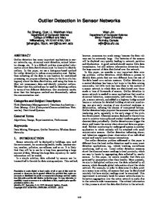
![Sensor ] ( Sensor](https://p.pdfkul.com/img/300x300/sensor-sensor_5a305cb11723ddc4471722ed.jpg)