Scalable K-Means by Ranked Retrieval
∗
Andrei Broder
Lluis Garcia-Pueyo
Vanja Josifovski
Google 1600 Amphitheater Parkway Mountain View, CA 94043
Google 1600 Amphitheater Parkway Mountain View, CA 94043
Google 1600 Amphitheater Parkway Mountain View, CA 94043
broder @google.com
[email protected]
[email protected]
Sergei Vassilvitskii
Srihari Venkatesan
Google 1600 Amphitheater Parkway Mountain View, CA 94043
xAd 440 North Wolfe Road Sunnyvale, CA 94085
[email protected] ABSTRACT
Categories and Subject Descriptors
The k-means clustering algorithm has a long history and a proven practical performance, however it does not scale to clustering millions of data points into thousands of clusters in high dimensional spaces. The main computational bottleneck is the need to recompute the nearest centroid for every data point at every iteration, a prohibitive cost when the number of clusters is large. In this paper we show how to reduce the cost of the k-means algorithm by large factors by adapting ranked retrieval techniques. Using a combination of heuristics, on two real life data sets the wall clock time per iteration is reduced from 445 minutes to less than 4, and from 705 minutes to 1.4, while the clustering quality remains within 0.5% of the k-means quality. The key insight is to invert the process of point-to-centroid assignment by creating an inverted index over all the points and then using the current centroids as queries to this index to decide on cluster membership. In other words, rather than each iteration consisting of “points picking centroids”, each iteration now consists of “centroids picking points”. This is much more efficient, but comes at the cost of leaving some points unassigned to any centroid. We show experimentally that the number of such points is low and thus they can be separately assigned once the final centroids are decided. To speed up the computation we sparsify the centroids by pruning low weight features. Finally, to further reduce the running time and the number of unassigned points, we propose a variant of the WAND algorithm that uses the results of the intermediate results of nearest neighbor computations to improve performance.
H.3.3 [Information Search and Retrieval]: Clustering
∗
Keywords k-means;WAND
1.
INTRODUCTION
The web abounds in high-dimensional “big” data: for example, collections such as web pages, web users, search clicks, and on-line advertising transactions. A common way to mitigate Bellman’s infamous “curse of dimensionality” [9] is to cluster these items: for example, classifying users according to their interests and demographics. Among popular approaches to clustering, the classic k-means algorithm remains a standard tool of practitioners despite its poor theoretical convergence properties [4, 34]. However, when clustering n data points into k clusters, each iteration of the k-means method requires O(kn) distance calculations, making it untenable for clustering scenarios requiring a partition of millions of points each with hundreds of non-null coordinates into thousands of clusters. While parallel programming techniques alleviate this cost by distributing the computation across many machines, with web scaled datasets, even massively parallelized implementation based on Hadoop (e.g. [16]) might take thousands of CPU-hours to converge on current hardware. Approaches optimizing the k-means running time generally fall into two categories: Some assume that the data is contained in a low dimensional space and use kd-trees and other geometric data structures to reduce the number of distance computations [21, 28, 29]; Others (e.g. [19, 30]) assume that the number of points per cluster is large, and subsample the data to deal with scale. Unfortunately when both the data dimensionality is high and the average number of points per cluster is small, both of the approaches above fail to provide significant speed ups. This is precisely the situation we address in this paper: we show how to reduce the cost of the k-means algorithm by large factors by adapting ranked retrieval techniques. Using a combination of heuristics, on two real-world data sets the wall clock time per iteration is reduced from 445 minutes to less than 4, and
Work done while the authors were at Yahoo! Research
Permission to make digital or hard copies of all or part of this work for personal or classroom use is granted without fee provided that copies are not made or distributed for profit or commercial advantage and that copies bear this notice and the full citation on the first page. Copyrights for components of this work owned by others than ACM must be honored. Abstracting with credit is permitted. To copy otherwise, or republish, to post on servers or to redistribute to lists, requires prior specific permission and/or a fee. Request permissions from
[email protected]. WSDM’14, February 24–28, 2014, New York, New York, USA. Copyright 2014 ACM 978-1-4503-2351-2/14/02 ...$15.00. http://dx.doi.org/10.1145/2556195.2556260 .
233
from 705 minutes to 1.4, without affecting quality or convergence speed—after 13 phases the algorithm has converged to within 0.5% of the k-means quality with the same number of phases. To reduce the cost of the k-means algorithm we use nearest neighbor data structures, optimized for retrieving the top ` closest points1 to a query point. Specifically, we use inverted indexes and a novel variant of the WAND ranked retrieval algorithm [12] to speed up the nearest centroid computations at the core of the k-means method. The k-means algorithm uses an iterative refinement technique where each iteration consists of two steps: the assignment step where the points are assigned to the closest centroid, and the update step where the centroids are recalculated based on the last assignment. The latter phase can be performed in a linear scan over the assigned points and is the less expensive of the two. Thus, we focus on the use of indexing to speed up point assignment. But what should we index? The natural choice is to index the centroids, and then run a query for each data point, retrieving the closest centroid. This approach would exactly implement the k-means algorithm, but since the centroids change in each iteration, this method requires both rebuilding the index and evaluating n queries at each iteration. In addition, as the centroids have many non-zero elements, they correspond to dense documents for which top-` nearest neighbor retrieval algorithms are not particularly efficient. In this work we propose the converse approach. Instead of indexing the centroids and using the points as queries, we propose indexing the points and using centroids as queries. This approach has several benefits. First, we do not need to rebuild the index between iterations since the points are stationary and only the centroids move from one iteration to the next. Second, the number of queries per iteration is significantly smaller (k rather than n) since we only pose one query per centroid. By retrieving only the top ` points closest to each centroid, we run the risk of leaving some points unassigned to any centroid. We show experimentally that the number of such points is low and thus they can be separately assigned once the final centroids are decided. In any case, these points are precisely the outliers in the dataset (they are far away from all known cluster centers), thus the setting of the parameter ` allows a tradeoff between the clustering speed and the acceptable number of outliers. Finally, in many applications, such as web search and ad selection, the application per se requires indexing the items of interest, thus large scale clustering of these items can be done without requiring significant additional infrastructure. To speed up the computation we begin by sparsifying the centroids by pruning low weight features: we show experimentally that this pruning brings significant improvements in efficiency while not changing the clustering performance at all. We then delve into the details of the WAND algorithm [12], and modify it to remember all of the points that were ranked in the top ` list during the retrieval. Again, our experimental evaluation over two datasets from realistic
practical scenarios shows that the proposed approaches are efficient and scale well with the number of clusters k, while having virtually no impact on the quality of the results. Indeed, in some cases, the new approaches produce clusters of slightly better quality than the standard k-means algorithm possibly by reducing the confusing effect of outliers. The techniques presented in this paper can be used in a single-machine setting, or at individual nodes in partitioned implementations. In both cases, the proposed method reduces the processing time and resource use by one to two orders of magnitude, while resulting in a negligible loss in clustering quality. In summary the contributions of this paper are as follows: • We describe an implementation of the k-means algorithm that is over 100 times faster than the standard implementation on realistic datasets by using an inverted index over all the points and then using the current centroids as queries into this index to decide on cluster membership. • We show experimentally that selectively re-assigning in each iteration only the subset of the points that are “close enough” to the current centroids and sparsifying the centroids does not materially change the quality of the final clustering. • For retrieval in the index above, we modify the WAND algorithm for similarity search to remember the runnerups in the current iteration and the radius of each cluster in the previous one, thus making significant efficiency gains.
2.
BACKGROUND
We follow the standard vector space model. Let T = {t1 , t2 , . . . , tm } be a collection of m terms, and D be a collection of n documents over the terms, D = {d1 , d2 , . . . , dn }. We treat each document d ∈ D as a vector lying in mdimensional term space, and use d(i) to denote the i-th coordinate. To judge the similarity between a pair of documents, we use the cosine similarity metric: for two documents d, d0 ∈ D: cossim(d, d0 ) =
d ◦ d0 , kdkkd0 k
where ◦ denotes the vector dot product, and k·k the vector’s length. Note that since the cossim measure is a function of the angle between the vectors d and d0 , it is invariant under scaling of its inputs. For any constants α, β > 0: cossim(d, d0 ) = cossim(αd, βd0 ). Thus we can assume without loss of generality that all of the documents d ∈ D are normalized to have unit length, kdk = 1. Recall that, the cossim of any pair of documents is always between 0 and 1, and f (d, d0 ) = 1 − cossim(d, d0 ) defines a metric: that is, it is non-negative, symmetric and satisfies the triangle inequality. Our goal is to find a partition of the documents in D into k non-overlapping clusters, C = {C1 , C2 , . . . , Ck } each with a representative point ci that maximizes the average cosine similarity between a document and its closest (under
1 we use the term top-` instead of top-k to avoid confusion between the number of retrieved points and the number of clusters in k-means clustering.
234
2.2
f ) representative. We will refer to the points ci as centers of individual clusters. Formally, we want to find a partition C which maximizes: X ψ(D, C) = max cossim(c, d). d∈D
2.1
c∈C
The k-means algorithm
The k-means algorithm is a widely used clustering method [24]. In its usual formulation, the algorithm is given a point set X ⊂ Rd , and a desired number of clusters k. It returns a set C of |C| = k cluster centers {c1 , . . . , ck } that forms a local minimum for a potential function X φ(X, C) = min kx − ck2 . x∈X
c∈C
In other words, it attempts to find a set of centers that minimizes the sum of squared distances between each point and its nearest cluster center. The algorithm is a local search method that minimizes φ by repeatedly (1) assigning each point to its nearest cluster center and (2) recomputing the best cluster centers given the point assignment.
K-means for Cosine Similarity We adapt the k-means algorithm to maximize the average cosine similarity, ψ. The assignment phase remains identical—we assign each point to the cluster center with the maximal cosine similarity. Next we show how to compute the optimal center given a set of points. To preserve the structure of the algorithm, we show below that selecting the (normalized) mean of the points as the center, maximizes the average similarity of a cluster. A similar observation has previously been made by Strehl et al. [32]. Lemma 1. For a set of n vectors D = {d1 , d2 , . . . , dn }, P i di P the unit length vector c = k di k maximizes i X cossim(c, d). d∈D
Proof. We want to find a unit length vector c that maximizes: X X X c◦d X = cossim(c, d) = c◦d=c◦ d kckkdk d∈D
d∈D
d∈D
d∈D
The vector c that maximizes the dot product with vector ¯ =P ¯ setting D d must be parallel to D, d∈D X 1 c= ¯ di kDk i
¯ and is of unit length. ensures that it is parallel to D Given the lemma, we can conclude that the k-means method will converge to a local optimum. Proposition 2. Given a set of documents D = {d1 , . . . , dn }, the k-means method which assigns each document to its most similar cluster, and recomputes the cluster center as the mean of the documents assigned to it converges to a local maximum of the objective function: X ψ(D, C) = max cossim(d, ci ) d∈D
c∈C
.
235
Ranked retrieval
Inverted indexes have become a de facto standard for evaluation of similarity queries across many different domains due to their very low latency and good scalability properties [35]. In an inverted index, each term t ∈ T has an associated postings list which contains all of the documents d ∈ D that contain t (those with d ∩ t 6= ∅). For each such document d, the list contains an entry called a posting. A posting is composed of the document id (DID) of d, and other relevant information necessary to evaluate the similarity of d to the query. In this paper we denote that additional information with d(t), and assume that it represents a weight for the particular term in the document. Such weights can be derived using variety of IR models [6] and in this work we chose to use the tf-idf weighting framework, but other methods are equally well applicable with our approach. The postings in each list are sorted in increasing order of DID. Often, B-trees or skip lists are used to index the postings lists, which facilitates searching for a particular DID within each list [35]. Inverted indexes are optimized for retrieving most similar documents for a query under an additive scoring model. Formally, a query q is a subset of terms, q ⊆ T , each with a given weight q(t). In this manner, a query can be seen as another document. Given a similarity function g, the score P of a document for a query, is t∈d∩q g(q(t), d(t)). When working with cosine similarity, the score is q ◦ d, with both q and d normalized to be unit length. Broder et al. [12] describe WAND, a method that allows for fast retrieval of the top-` ranked documents for a query. We choose WAND due to its ability to scale well with the number of features in the query, as reported in [15]. Additionally, this is a method where we can use information from previous rounds to further improve the retrieval time. A major difference in our setting is the fact that queries, representing centroids in k-means, are dense. We take special measures to sparsity the vectors, nevertheless, in our work queries are still substantially longer than the average search query of approximately 3 words. The main intuition behind the WAND algorithm (presented in Algorithm 1) is to use an upper bound of the similarity contribution of each term to eliminate documents that are too dissimilar from the query to make it into the top-` list. WAND works by keeping one pointer called a cursor for each of the query terms (dimensions) that points at a document in the corresponding posting list. During the evaluation, the algorithm repeatedly choses a cursor to be moved, and advances this cursor as far as possible in order to avoid examining unnecessary documents. To find the optimal cursor and improve the efficiency, the cursors are kept sorted by the DID they point to. At initialization time, for each term t ∈ T , WAND first fetches the upper bound UBt of the document weights across all documents in the posting list of t. UBt is query independent and is computed and stored during the index building phase at no extra cost. Next, all cursors are initialized by pointing at the first posting in their corresponding posting lists (the one with the minimum DID). The outer loop of the algorithm repeatedly retrieves the next (in order of DID) document that qualifies for the top-` list.
Algorithm 2 FindCandidate 1: Input: Query: q Cursors[1..|q|]: array of cursors over the posting lists used in the query, Threshold: θ 2: Output: Next feasible document, its similarity 3: loop 4: {Find pivot cursor} 5: pivotTerm ← findPivotTerm(Cursors,θ) 6: if pivotTerm == Null then 7: return N oM oreDocs 8: end if 9: pivotDoc ← Cursors[pivotTerm].DID 10: if Cursors[0].DID == pivotDoc then 11: {Evaluate pivot document} 12: if cossim(q,pivotDoc) ≥ θ then 13: return pivotDoc, cossim(q, pivotDoc) 14: end if 15: else 16: {Advance Cursors} 17: dim ← PickCursor(Cursors[0..pivotTerm]) 18: Cursors[dim].advance(pivotDoc) 19: end if 20: end loop
During the evaluation, the algorithm maintains a heap of highest scoring top-` documents among those examined so far. The minimum score in this heap, or the score of the current `-th best result, is denoted by θ. The key property of WAND is that it does not fully score every document, but skips the ones that have no chance in making it in the top-` list. Intuitively, if we can determine that the score of a an unexamined document cannot be higher than θ, then we can forego any further evaluation of this document and skip to the next DID that has a chance at success. The first document that has the property of having upper bound of its score higher than θ is known as the pivot document. We present the pivot finding subroutine as Algorithm 2. The subroutine relies on two helper functions. The first, findPivotTerm, returns the earliest term, t∗ , in the list, such that the sum of the score upper bounds, UBt for all terms t preceding t∗ is at least θ. Given the pivot document, we then check whether the cursors in the first and t∗ -th position point to the same document. Since the cursors are sorted by DID, if the two cursors point to different documents, the one pointed to by the first cursor cannot possibly make it to the top-` list. and we advance the cursors (Lines 15-18). The function PickCursor selects a cursor to advance to the first document with DID at least d∗ (Line 17). On the other hand, If both the first cursor and the cursor at t∗ point to a posting with the same DID, the similarity of that document is fully evaluated (Line 12). In the description we have simplified the algorithm by not dealing with some of the stopping conditions and end of postings list issues. The WAND algorithm is fully described in [12]. We have also described a basic version of the WAND algorithm for simplicity: several modifications are possible to improve the efficiency of the processing both for on-disk and in-memory scenarios [15].
we mentioned previously, the main bottleneck in getting kmeans to work on millions of points and thousands of clusters in multi-thousand dimensional spaces is the fact that at every iteration we must find the nearest cluster center to every one of the data points. The naive implementation requires O(nkd) time per round. Previous work has focused on reducing this complexity either by sampling ([19, 30]), which does not work well when the number of points per cluster is relatively small, or by employing kd-trees and other data structures ([21, 28, 29]) which are only efficient in low dimensional spaces. A simple approach to reduce the amount of time to compute the nearest cluster center for every point would be to build a nearest neighbor data structure on the cluster centers, and then issue a query for each data point to find the nearest neighbor. Unfortunately since the cluster centers move at every iteration this would force us to rebuild the index at every iteration, the cost of which would outweigh any potential savings. Instead we perform the converse. We build a nearest neighbor data structure on the points and then use the current centroids as queries to find the points closest to the centroids. Since the points do not move from one iteration to the next, we only have to build the index once, thereby amortizing the cost across the iterations of kmeans. Furthermore, often, inverted indexes of the points are build for other applications and can be reused for the computation of the clusters, using the algorithms described in this section. This approach has an additional benefit: it automatically detects outliers. Intuitively, the outlier points are precisely those points that are far away from all of the centers, and with this method these are exactly the points that are never returned by the nearest neighbor data structure. It is well known [18] that outliers present a problem for k-means and
Algorithm 1 WAND 1: Input: Centroid query C Index I 2: Output: Heap H with the top ` points most similar to C 3: for t ∈ dimensions(C) do 4: fetch UBt 5: Cursors[t].DID = first DID in posting list(t); 6: end for 7: Initialize empty heap H of size `; 8: while true do 9: sort Cursors by Cursors[t].DID (ascending) 10: θ = minSimilarity(H) 11: (candidate, sim) = F indCandidate(Cursors, θ); 12: if candidate == LastDID then 13: break; 14: end if 15: replaceM inElement(H, candidate, sim); 16: end while 17: return H;
3.
ALGORITHMS
In this Section we describe our main approach of using an inverted index to speed up k-means computations. As
236
can skew the position of the final clusters. In our algorithm, the outliers are never be retrieved as part of the top-` list for any of the centroids, therefore they do not impact the computation, rather we assign them to clusters in a post processing step. The value of the parameter ` allows us to control the rank (number of closer points) that classifies a point into an outlier.
3.1
in iteration t would also qualify for iteration t+1. (A similar approach was used by Elkin [14] to reduce the number of distance computations performed by k-means.) This follows by the fact that 1 − cossim forms a metric, thus for any point d: cossim(d, ct+1 ) ≥ cossim(d, cti ) − cossim(ct+1 , cti ) i i ≥ θit − σit = θit+1
WAND Based k-means
We present a progression of algorithms that incorporate the nearest neighbor index into k-means.
In practice, we find that setting θit+1 = θti works equally well and is more efficient, since we can forgo the computation of σit .
WAND for point assignment
Expanded use of the assignment table
The first algorithm we explore uses standard WAND to perform the point assignment as described in Section 2. Instead of the nested loop computing the distances for all pairs of centroids and points, as in regular k-means, we invoke the WAND algorithm to find the top-` closest points to each centroid. The WAND operator returns a set of ` points along with their similarity to the cluster. Although these are the most similar ` documents to the center, a single document d may be in the top-` lists for a number of different centroids. Thus we have to maintain the id of the centroid that is closest to d. We proceed by using an assignment table A which is a map with the document id, DID, as the key and whose payload contains the id of the most similar center and the corresponding similarity. Each point returned by the WAND operator is then checked against this table. If it is already in the table with a similarity larger than the one returned for the current cluster, the result is ignored. Otherwise it is added to the table with the new similarity, potentially replacing an existing entry associated with a previously evaluated centroid. The assignment table is reset at the beginning of each iteration.
By pushing the assignment table into the WAND subroutine, the caller only has access to the final Di documents returned. However, during the course of computing the top-` documents most similar to ci , the full similarity is computed for many more documents. There are two reasons why this similarity may not be preserved. First, a document may be reassigned to an even closer center in the assignment table, A. However, it could also be the case that a document d lies in the Voronoi cell of a particular centroid ci (that is it is closer to ci than to any other centroid), but it is not one of the top-` documents closest documents. If such a document d has a low DID then it will be fully scored, and temporarily placed on the heap in WAND, only to be replaced by an even closer document later on. As we show below, this situation is far from rare, and remembering the assignment and similarity information for such documents allows the algorithm designer to set a lower threshold ` to achieve the same effect. Therefore it pays to remember this information and incorporate it when computing the centroids. The final version of the wand-k-means algorithm, shown in Algorithm 3
Using the assignment table within WAND
3.2
Instead of using the assignment table A to post-process the results returned by WAND, we may instead modify the WAND algorithm to use the table A directly. The corresponding similarity value in A then serves as a lower bound on the similarity a point must achieve in order to be returned by WAND. TWe omit the full specification of this algorithm for brevity.
The key idea behind the algorithms presented thus far is to consider only the `-closest points to the cluster center when executing the assignment phase of k-means. To find the ` closest points, the WAND algorithm gains added efficiency by giving up on the distance computation as soon as one can safely conclude that the point is further away than the desired threshold. Nevertheless, during the typical course of its operation, the exact distance is computed for more than ` points. We formally analyze the number of such points and show it to be significantly higher than `. Consider a point set D = {d1 , d2 , . . . , dn }, a center c and let the elements of D be examined in a random order. The question we consider is how many elements of D are ever included in the top-` list. Call such an element d ∈ D fullyexamined.
Warm start of thresholds The WAND algorithm works by comparing the partial score of documents to the score of the `-th best result. In the naive implementation as in Algorithm 2, this threshold, θ is initialized to 0 at every iteration. This has the effect that the first ` documents are always fully evaluated, since their similarity is guaranteed to be at least 0. We can improve the performance by keeping track of intermediate information across the k-means iterations. Specifically, for each cluster ci we remember the threshold, θit , used by WAND when executed with cti as the query at time t (this is identical to the similarity to the `-th closest point considered by WAND). Let σit denote the similarity between the center of cluster i at time t and that at time t−1. Then if we set the threshold in the following iteration to θit+1 = θit − σti , we can guarantee that all of the points returned by WAND
Analysis
Lemma 3. If D is examined in a random order, the expected number of fully examined points is `(1+log n` )+o( n` ). Proof. A point di ∈ D is fully examined if and only if it is one of the `-closest points to c among those in {d1 , d2 , . . . , di }. Let Yi be an indicator variable which is set to 1 if the point in position i is fully examined and 0 otherwise and let pi denote the probability that yi is set to P1. Then the P expected number of fully examined points is i E[Yi ] = i pi .
237
Algorithm 3 wand-k-means 1: wand-k-means: 2: Input: D = Set of documents, k 3: Output: Centroids, C = {c1 , . . . , ck } 4: φ = ∞ 5: C ← InitializeCentroids 6: θ[1..k] ← 0 7: repeat 8: φ∗ ← φ, φ ← 0, A ← ∅ 9: for all ci ∈ C do {Find Nearby Documents} 10: hA, θi i ← WAND(ci , i, A, `, θi ) 11: end for 12: for 1 ≤ i ≤ k do {Compute Assignment} 13: Ci ← {d ∈ D : A[d].clust = i} 14: end for 15: for 1 ≤ i ≤ P k do {Recompute Centers} 16: ci ← |C1i | d∈Ci d 17: for all d ∈ Ci do {Update Cost Function} 18: φ ← φ + A[d].sim 19: end for 20: end for 21: until φ = φ∗ 22: return C = {c1 , . . . , ck }
In practice the order of the documents in D is not random, but we can use the intuition given by the Lemma to show that even when looking for the ` closest points, the algorithm will compute the distances to far more than ` points, which in turn allows us to use WAND with a smaller value of `, improving its performance.
1: 2: 3: 4: 5: 6: 7: 8: 9: 10: 11: 12: 13: 14: 15: 16: 17: 18:
The majority of time in any implementation of the kmeans algorithm is spend computing the cosine similarity between two points. As we saw in the previous section, we can leverage the infrastructure initially designed for nearest neighbor retrieval to improve the speed of k-means. The inverted index data structure that we use for nearest neighbor retrieval is especially efficient in the case that the query itself is sparse, i.e. contains few non-zero entries. In the applications we consider, the points (or documents) lie in a very high dimensional space: for example, the datasets in our experiments consist of 26 million and 7 million features respectively. Although an individual document typically has a small number of features (we find the average number of features per document to be around 100), the number of features in the cluster center ci tends to be very large, since the cluster center almost surely has a non-zero value for every feature present in the individual documents. As an additional optimization, we consider sparsifying each cluster center after computing it, effectively only keeping the top p features with the highest absolute value. A similar performance improvement was previously suggested in [30], the combination of sparse clusters with inverted indexing further improves the performance gained by this approach.
3.2.1
3.3
WAND Input: query q, cluster id i, table A, `, threshold θi Output: updated table A for all i ∈ q do Cursors[i].init end for H ← Heap of size ` while true do θi ← max(θi , min(H)) hd, simi ←WAND-Next(Cursors, θi ) if d == null then return A end if if (A[d] == null or A[d].sim < sim) then A[d].sim ← sim, A[d].clust ← i H.add(sim) end if end while
Since the first ` points are always examined, for 1 ≤ i ≤ ` we have pi = 1. Now consider a point in position j > `, it will be fully examined only if it is one of the ` closest points among those in positions 1, 2, . . . , j. Since we assumed that the elements arrived in random order, pj = j` . Therefore, n X i=1
pi = ` +
n X i=`+1
pi = ` +
Convergence
The original k-means algorithm increases the overall similarity in every step—both when assigning each point to its most similar center, and when recomputing the centers. Therefore, it is well known that it will converge to a locally optimum solution, although such convergence may take an exponential number of steps [34]. Since the wand-k-means algorithm potentially examines only the closest ` points in each iteration, the same analysis no longer holds. To ensure convergence, we compute the cost of assigning all of the points every 50 iterations, and stop if no progress is made on this objective. As we will show, in practice the algorithm keeps all of the convergence properties of k-means: it converges to a locally optimum solution after just a handful of iteration, see Section 4 for more details.
4.
Sparsification
EXPERIMENTAL EVALUATION
In this Section we present the results of the empirical evaluation of the algorithms on two real-world datasets. We begin by describing the datasets, and then evaluate the effect of each of the parameters. We use two datasets from a real world textual advertising system. In Dataset 1, each point (item) represents a textual ad (encompassing both sponsored search and content match) from a production version of a large internet search engine in 2008. The point features are extracted from the combination of the ad creative (the body, title, display url) and the list of keywords that the advertisers have associated with the
n X ` = `(1 + Hn − H` ) i
i=`+1
1 = `(1 + log n − log ` + o( )) n n ` = `(1 + log ) + o( ) ` n
238
!"#$$%&"'()(*+,-'".$)2'0)%.'0#1*")
ad. Clustering of similar ads is used in a variety of textual advertising tasks, for example to predict the clickthrough rate of previously unseen ads. Dataset 2 is composed of web search queries that are expanded with features of the web search results returned by a search engine. It is well known that the brevity of the queries poses a challenge in query analysis and it is beneficial to expand them. Such an approach has been shown to work well for classification [11]. The queries in Dataset 2 were chosen by a stratified sampling of web queries by volume. The main statistics of the two datasets are provided in Table 1.
+!!!"
*!!!"
)!!!"
!"#$$%&"'()(*+,-'".$)
(!!!"
'!!!" ,-./01023-.45"67'!!" ,-./01023-.45"67#!!"
&!!!"
,-./01023-.45"67#!" ,-./01023-.45"67#"
%!!!"
$!!!"
Number of Documents Number of Features Average Features per Document
Dataset 1 974,738 26,013,163 95.6
Dataset 2 933,761 7,126,669 98.9
#!!!"
!" #"
%#"
&#"
'#"
(#"
Figure 3:
The number of unassigned documents in Dataset 1 as a function of the number of iterations for different values of `.
Initialization
There are two initialization tasks that must be performed before running the wand-k-means algorithm, building the index and selecting the initial centers. Building the index took approximately 54 minutes on both of the datasets above. In order to make for a fair comparison between methods, we computed an initial seed set for both datasets and then used the same initial seeds in all of the algorithms and baselines. We used k-means++ [5] as the initialization method, as it has been proven to perform significantly better than a simple random assignment both in theory and in practice. We chose to cluster the data into k = 1000 clusters for the majority of the experiments. We report on scalability experiments separately in Section 4.4.
4.1
$#"
/.'0#1*")
Table 1: Dataset statistics.
4.0.1
##"
clustering. In Figure 1(b) we plot the average time per iteration. It is clear that by reducing the value of ` we reduce the per iteration running time of k-means more than five-fold.
4.2
Outliers
We further explore the trade-off between the setting of the parameter ` and the number of documents marked as unassigned by the algorithm. Recall, the unassigned documents are those that do not appear in the top-` list any cluster center during the execution of WAND. We plot the number of unassigned documents as a function of the iteration in Figure 3. There are two interesting observations. First, as expected, reducing ` allows wand-k-means to label more points as outliers, and the algorithm does take advantage of this new freedom. Moreover, the set of outliers remains very small, even the 6,500 outliers at ` = 1, represent less than 1% of the overall dataset.
Number of documents retrieved
The overall results are shown in Table 2, where we evaluate all the average similarity, ψ for all of the methods at iteration 13. The average similarity is computed after assigning all of the documents to their nearest center. As we can see, decreasing ` has a negligible effect on the final clustering similarity, but tremendously speeds up the iteration time. The effect of using all of the documents fully examined by WAND is apparent as well, even the setting of ` = 1 performs very well, owning to the fact that many more documents are examined during the WAND iteration. In addition, smaller values of ` allow wand-k-means to converge to a slightly better optimum than the vanilla kmeans method. We conjecture that this is due to the fact that outliers are automatically detected and ignored during the execution of the algorithm (since they are not part of the top ` elements). By changing the value of ` we do not affect the rate of convergence to the final solution. In Figure 1(a) we plot the average similarity as a function of the number of iterations. Here, we only compute the similarity for those documents that are assigned to some cluster at each iteration, but as we will see later (Section 4.2) the total number of unassigned documents is rather small. The rate of convergence to a solution does not change as a function of `, and examining fewer points has no detrimental effects on the quality of the
4.3
Sparsification
In this section we investigate the effect of the sparsification parameter p on the algorithm’s performance. We present the overall results, showing the average similarity of all documents at the end of iteration 13 in Table 3. Note that, while generally decreasing p slowly decreases the quality of the clustering, high values of p perform much better than having no sparsification at all. Again, we conjecture that this is because sparsification allows the algorithm to focus its performance on the critical features and ignore the contributions of outliers to the centroids. The effect of p on the running time is even larger than that obtained by restricting `. By insisting that the centroid have at most 500 non-zero features reduces the running time by a factor of 7 for dataset 1, and over a factor of 60 for dataset 2. The performance increase is much bigger for dataset 2, because the average similarity is low, and thus WAND is less effective at pruning out far away documents. To study the effect of sparsification on convergence, we again plot the per iteration quality and running time in Figure 2(a) and 2(b) respectively. (Here too we only compute
239
System k-means wand-k-means wand-k-means wand-k-means
` — 100 10 1
Dataset 1 Similarity 0.7804 0.7810 0.7811 0.7813
Dataset 1 Time 445.05 83.54 75.88 61.17
Dataset 2 Similarity 0.2856 0.2858 0.2856 0.2709
Dataset 2 Time 705.21 324.78 243.9 100.84
Table 2: The average point to centroid similarity at iteration 13 and average iteration time (in minutes) as a function of ` . /0+&%1+)!"#"$%&"'()2+&)*'+&%,-.)
!"#$%/$+%"*$+,-.'%
!"#(
%$$!!"!!#
!"#(%
($!"!!#
(!!"!!#
!"#'
%$'$!"!!#
!"#'%
!"#$%&#"'(%
!"#"$%&"'()
'!!"!!#
!"##$% -./0123% 4125.-./01236%78)!!%
!"##%
4125.-./01236%78)!%
+,-./01#
&$!"!!#
2/03,+,-./014#56%!!# 2/03,+,-./014#56%!#
&!!"!!#
4125.-./01236%78)%
2/03,+,-./014#56%#
!"#&$% %$!"!!#
!"#&%
%!!"!!#
!"#$
%$$!"!!#
!"#
%$!"!!#
)%
))%
*)%
+)%
,)%
$)%
&)%
#)%
%#
%%#
&%#
'%#
*'+&%,-.)
(%#
$%#
)%#
*%#
)*$+,-.'%
(a)
(b)
Figure 1: Evaluation of wand-k-means on Data 1 as function of different values of `: (a) The average point to centroid similarity at each iteration (b) The running time per iteration. /0+&%1+)!"#"$%&"'()2+&)*'+&%,-.)
!"#$%/$+%"*$+,-.'%
!"#(
%$($"!!#
!"#(% (!"!!# !"#'
%$'"!!#
!"##
%$!"#$%&#"'(%
!"#"$%&"'()
!"#'%
-./0123% 4125.-./01236%78$!% 4125.-./01236%78)!!%
!"##%
,-./01023-.45#67*!#
&"!!#
,-./01023-.45#67(!!# ,-./01023-.45#67$!!#
4125.-./01236%78*!!%
,-./01023-.45#67*!!#
4125.-./01236%78$!!%
!"#&
%$%"!!#
!"#&% $"!!# !"#$
%$!"#
%$!"!!# )%
))%
*)%
+)%
,)%
$)%
&)%
#)%
(#
*'+&%,-.)
((#
$(#
)(#
%(#
*(#
&(#
+(#
)*$+,-.'%
(a)
(b)
Figure 2: Evaluation of wand-k-means on Dataset 1 as a function of different values of p: (a) The average point to centroid similarity at each iteration (b) The running time per iteration. Note that we de not display the running time of k-means in part (b) since it is over 50 times slower.
4.4
the similarity for those documents that are assigned to some cluster at each iteration.) Note that we removed the running time of k-means from Figure 2(b) since it is almost two orders of magnitude worse than all of the other methods.
Number of Clusters
Next we investigate the performance of the algorithm as we increase the number of clusters, k beyond to 3,000 and 6,000.
240
System k-means wand-k-means wand-k-means wand-k-means wand-k-means wand-k-means
p — — 500 200 100 50
` — 1 1 1 1 1
Dataset 1 Similarity 0.7804 0.7813 0.7817 0.7814 0.7814 0.7803
Dataset 1 Time 445.05 61.17 8.83 6.18 4.72 3.90
` — 10 10 10 10 10
Dataset 2 Similarity 0.2858 0.2856 0.2704 0.2855 0.2853 0.2844
Dataset 2 Time 705.21 243.91 4.00 2.97 1.94 1.39
Table 3: Average point to centroid similarity and iteration time (minutes) at iteration 13 as a function of p . duce. The all point similarity algorithm proposed in [8] also uses indexing but focuses on savings achieved by avoiding the full index construction, rather than repeatedly using the same index in multiple iterations. Yet another approach has been suggested by Sculley [30], who showed how to use a sample of the data to improve the performance of the k-means algorithm. Similar approaches were previously used by Jin et al. [19]. Unfortunately this, and other subsampling methods break down when the average number of points per cluster is small, requiring large sample sizes to ensure that no clusters are missed. Finally our approach is related to subspace clustering [27] where the data is clustered on a subspace of the dimensions with a goal to shed noisy or unimportant dimensions. In our approach we perform the dimension selection based on the centroids and in an adaptive manner, while executing the clustering approach. In our current work we are exploring more the relationship between our approach and some of the reported subspace clustering approaches. Indexing. A recent survey and a comparative study of in-memory Term at a time (TAAT) and document at a time (DAAT) algorithms was reported in [15]. A large study of known TAAT and DAAT algorithms was conducted by [22] on the Terrier IR platform with disk-based postings lists using TREC collections They found that in terms of the number of scoring computations, the Moffat TAAT algorithm [26] had the best performance, though it came at a tradeoff of loss of precision compared to naive TAAT approaches and the TAAT and DAAT M AXSCORE algorithms [33]. In this paper we did not evaluate approximate algorithms such as Moffat TAAT [26]. We leave this study as future work. Finally, a memory-efficient TAAT query evaluation algorithm was proposed in [23].
We observe the same qualitative behavior: the average similarity of wand-k-means is indistinguishable from k-means, while the running time is faster by an order of magnitude.
5.
RELATED WORK
Clustering. The k-means clustering algorithm remains a very popular method of clustering over 50 years after its initial introduction by Lloyd [24]. Its popularity is partly due to the simplicity of the algorithm and its effectiveness in practice. Although it can take an exponential number of steps to converge to a local optimum [34], in all practical situations it converges after 20-50 iterations (a fact confirmed by the experiments in Section 4). The latter has been partially explained using smoothed analysis [3, 5] to show that worst case instances are unlikely to happen. Although simple, the algorithm has a running time of O(nkd) per iteration, which can become large as either the number of points, clusters, or the dimensionality of the dataset increases. The running time is dominated by the computation of the nearest cluster center to every point, a process taking O(kd) time per point. Previous work, [14, 20] used the fact that both points and clusters lie in a metric space to reduce the number of such computations. Other authors [28, 29] showed how to use kd-trees and other data structures to greatly speed up the algorithm in low dimensional situations. Since the difficulty lies in finding the nearest cluster for each of the data points, we can instead look for nearest neighbor search methods. The question of finding a nearest neighbor has a long and storied history. Recently, locality sensitive hashing, LSH [2] has gained in popularity. For the specific case of document retrieval, inverted indices [6] are the state of the art. We note that a straightforward application of both of these approaches would require rebuilding the data structure and querying it n times during every iteration, thereby negating most, if not all, of the savings over a straightforward naive implementation. The well known data deluge lead several groups of researchers to investigate the k-means algorithm in the regime when the number of points, n is very large. Guha et al. [17] show how to solve k-clustering problems in a data stream setting where points arrive incrementally one at a time. Their analysis for the related k-median problem was further refined and improved by [13, 25] and most recently by [10, 31]. However, all of these methods scale poorly with k, which is the problem we tackle in this work. As parallel algorithms have reemerged in their popularity these methods were adapted to speeding up k-means as well, [1, 7]. In fact the k-means method is implemented in Mahout [16], a popular machine learning package for MapRe-
6.
CONCLUSION
In this work we showed that using centroids as queries into a nearest neighbor data structure built on the data points can be very effective in reducing the number of distance computations needed by the k-means clustering method. Additionally, we showed that using the full information from the WAND algorithm, and sparsifying the centroids further improves performance. Our experimental evaluation over two real world data sets shows that the approach proposed in this paper is viable in practice, with up to a 20x reduction in the computation time, especially for large values of k.
7.
REFERENCES
[1] N. Ailon, R. Jaiswal, and C. Monteleoni. Streaming k-means approximation. In Y. Bengio, D. Schuurmans,
241
[2]
[3]
[4]
[5]
[6]
[7]
[8]
[9] [10]
[11]
[12]
[13]
[14] [15]
[16]
[17] [18]
J. Lafferty, C. K. I. Williams, and A. Culotta, editors, NIPS 22. 2009. A. Andoni and P. Indyk. Near-optimal hashing algorithms for approximate nearest neighbor in high dimensions. Commun. ACM, 51(1):117–122, Jan. 2008. D. Arthur, B. Manthey, and H. R¨ oglin. Smoothed analysis of the k-means method. J. ACM, 58(5):19, 2011. D. Arthur and S. Vassilvitskii. How slow is the k-means method? In Symposium on Computational Geometry, 2006. D. Arthur and S. Vassilvitskii. K-means++: the advantages of careful seeding. In N. Bansal, K. Pruhs, and C. Stein, editors, SODA. SIAM, 2007. R. A. Baeza-Yates and B. Ribeiro-Neto. Modern Information Retrieval. Addison-Wesley Longman Publishing Co., Inc., Boston, MA, USA, 1999. B. Bahmani, B. Moseley, A. Vattani, R. Kumar, and S. Vassilvitskii. Scalable k-means++. PVLDB, 5(7):622–633, 2012. R. J. Bayardo, Y. Ma, and R. Srikant. Scaling up all pairs similarity search. In Proceedings of the 16th international conference on World Wide Web, WWW ’07, 2007. R. E. Bellman. Dynamic Programming. Princeton University Press, Princeton, NJ, USA, 1957. V. Braverman, A. Meyerson, R. Ostrovsky, A. Roytman, M. Shindler, and B. Tagiku. Streaming k-means on well-clusterable data. In Proceedings of the Twenty-Second Annual ACM-SIAM Symposium on Discrete Algorithms, SODA ’11, pages 26–40. SIAM, 2011. A. Broder, M. Fontoura, E. Gabrilovich, A. Joshi, V. Josifovski, and T. Zhang. Robust classification of rare queries using web knowledge. In SIGIR’07, 2007. A. Z. Broder, D. Carmel, M. Herscovici, A. Soffer, and J. Y. Zien. Efficient query evaluation using a two-level retrieval process. In CIKM, 2003. M. Charikar, L. O’Callaghan, and R. Panigrahy. Better streaming algorithms for clustering problems. In L. L. Larmore and M. X. Goemans, editors, STOC. ACM, 2003. C. Elkan. Using the triangle inequality to accelerate k-means. In ICML, pages 147–153, 2003. M. Fontoura, V. Josifovski, J. Liu, S. Venkatesan, X. Zhu, and J. Y. Zien. Evaluation strategies for top-k queries over memory-resident inverted indexes. PVLDB, 4(11), 2011. A. S. Foundation, I. Drost, T. Dunning, J. Eastman, O. Gospodnetic, G. Ingersoll, J. Mannix, S. Owen, and K. Wettin. Apache mahout, 2010. http://mloss.org/software/view/144/. S. Guha, N. Mishra, R. Motwani, and L. O’Callaghan. Clustering data streams. In FOCS, 2000. V. Hautam¨ aki, S. Cherednichenko, I. K¨ arkk¨ ainen, T. Kinnunen, and P. Fr¨ anti. Improving k-means by outlier removal. In SCIA, 2005.
[19] R. Jin, A. Goswami, and G. Agrawal. Fast and exact out-of-core and distributed k-means clustering. Knowl. Inf. Syst., 10(1):17–40, July 2006. [20] T. Kanungo, D. M. Mount, N. S. Netanyahu, C. D. Piatko, R. Silverman, and A. Y. Wu. An efficient k-means clustering algorithm: Analysis and implementation. IEEE Trans. Pattern Anal. Mach. Intell., 24(7), 2002. [21] T. Kanungo, D. M. Mount, N. S. Netanyahu, C. D. Piatko, R. Silverman, and A. Y. Wu. A local search approximation algorithm for k-means clustering. Comput. Geom., 28(2-3), 2004. [22] P. Lacour, C. Macdonald, and I. Ounis. Efficiency comparison of document matching techniques. In Efficiency Issues in Information Retrieval Workshop; European Conference for Information Retrieval, 2008. [23] N. Lester, A. Moffat, W. Webber, and J. Zobel. Space-limited ranked query evaluation using adaptive pruning. In WISE, 2005. [24] S. P. Lloyd. Least squares quantization in pcm. IEEE Transactions on Information Theory, 28, 1982. [25] A. Meyerson. Online facility location. In FOCS, 2001. [26] A. Moffat and J. Zobel. Self-indexing inverted files for fast text retrieval. ACM Transactions on Information Systems, 14(4), 1996. [27] L. Parsons, E. Haque, and H. Liu. Subspace clustering for high dimensional data: a review. SIGKDD Explor., 6(1), 2004. [28] D. Pelleg and A. Moore. Accelerating exact k-means algorithms with geometric reasoning. In Proceedings of the fifth ACM SIGKDD international conference on Knowledge discovery and data mining, KDD ’99, pages 277–281, New York, NY, USA, 1999. ACM. [29] D. Pelleg and A. Moore. X-means: Extending k-means with efficient estimation of the number of clusters. In In Proceedings of the 17th International Conf. on Machine Learning, pages 727–734. Morgan Kaufmann, 2000. [30] D. Sculley. Web-scale k-means clustering. In WWW, 2010. [31] M. Shindler, A. Wong, and A. W. Meyerson. Fast and accurate k-means for large datasets. In J. Shawe-Taylor, R. Zemel, P. Bartlett, F. Pereira, and K. Weinberger, editors, Advances in Neural Information Processing Systems 24, pages 2375–2383. 2011. [32] A. Strehl, J. Ghosh, and R. J. Mooney. Impact of similarity measures on web-page clustering. In Proc. AAAI Workshop on AI for Web Search (AAAI 2000), Austin, pages 58–64. AAAI/MIT Press, July 2000. [33] H. R. Turtle and J. Flood. Query evaluation: Strategies and optimizations. Information Processing and Management, 31(6), 1995. [34] A. Vattani. k-means requires exponentially many iterations even in the plane. Discrete & Computational Geometry, 45(4):596–616, 2011. [35] J. Zobel and A. Moffat. Inverted files for text search engines. ACM Computing Surveys, 38(2), 2006.
242