Scalable Community Discovery from Multi-Faceted Graphs Ahmed Metwally Jia-Yu Pan Minh Doan Google Inc. 1600 Amphitheatre Pkwy, Mountain View, CA 94043 {metwally, jypan, minhdoan}@google.com Abstract—A multi-faceted graph defines several facets on a set of nodes. Each facet is a set of edges that represent the relationships between the nodes in a specific context. Mining multi-faceted graphs have several applications, including finding fraudster rings that launch advertising traffic fraud attacks, tracking IP addresses of botnets over time, analyzing interactions on social networks and co-authorship of scientific papers. We propose NeSim, a distributed efficient clustering algorithm that does soft clustering on individual facets. We also propose optimizations to further improve the scalability, the efficiency and the clusters quality. We employ generalpurpose graph-clustering algorithms in a novel way to discover communities across facets. Due to the qualities of NeSim, we employ it as a backbone in the distributed MuFace algorithm, which discovers multi-faceted communities. We evaluate the proposed algorithms on several real and synthetic datasets, where NeSim is shown to be superior to MCL, JP and AP, the well-established clustering algorithms. We also report the success stories of MuFace in finding advertisement click rings.
I. Introduction A multi-faceted graph, a.k.a multi-graph, defines several facets on the same set of nodes. Each facet comprises edges that represent the relationship between nodes in a specific context. This is a more realistic representation of complex relationships between natural entities than a single graph. Our main motivation is to find ad fraud rings [28], i.e., a group of online content publishers conducting advertising traffic fraud [8]. Several Internet services such as web search, web mail, social networks, maps, and others are provided to the public free of charge. This is often possible due to the revenue generated by Internet advertising, an industry that in 2014 generated over 50 billion USD in the U.S. alone [7]. In online advertising, a publisher registers its web sites with the network operator, e.g., Google, to display ads on his/her sites. Publishers receive revenue to a designated payment instrument, e.g., bank account, for actions on the displayed ad, e.g., viewing or clicking the ad by a site visitor. Without loss of generality, we limit the discussion to cost-per-click advertising where the revenue is generated for each ad click. Dishonest publishers launch surges of fake clicks, a.k.a. click fraud attacks, on ads hosted by their own websites to inflate their revenue. Google has invested much effort to protect advertisers from such attacks [24, 37]. To circumvent these efforts and stay under the radar level, a fraudster may sign up for multiple accounts to spread the revenue.
Christos Faloutsos Carnegie Mellon University 5000 Forbes Avenue, Pittsburgh, PA 15213
[email protected] Each publisher has meta-data, i.e., account attributes. Clustering publisher accounts that are related on one attribute is a viable way to discover potential click rings. Some attributes have proved to have higher accuracy than others, where accuracy is the ratio of the identified clusters that are truly fraudulent click rings, based on manual reviews. For instance, clustering the publishers based to the IP addresses (IPs) that generate the clicks on their websites was reported to be highly accurate in catching click rings [28]. However, more sophisticated click rings often comprise publishers that are not related by accurate attributes. We propose catching click rings by clustering publishers on multiple corroborative attributes even if they have lower accuracy. This motivates analyzing a multi-graph where the nodes represent publisher accounts, and each facet contains the edges representing pairs of publishers that are similar on a specific attribute. Another application of multi-graphs is modeling timeevolving graphs1 . An illustrative example is tracking the IP addresses (IPs) used by click botnets [9]. To avoid having their IPs blacklisted, it is typical of click botnets to gradually change the attacking behavior and the attacking IPs over time [44]2 . Still, a botnet can be tracked over time by detecting the attacking IPs at consecutive snapshots. To that end, we propose forming a multi-faceted graph from different snapshots, where each node represent an IP, each facet represent a snapshot, and an edge between two IPs at a snapshot exist if the two IPs click similar sets of publishers’ pages. IPs can be clustered within each facet, and clusters can be correlated across facets. Hence, botnet-IPs can be tracked over time even if the attacking IPs change and the behavior of the IPs evolve over time. Multi-graphs have several other applications, such as interaction on social networks. A person participates in multiple networks of different social functions (e.g., professional, geographic, academic, or hobby). These interactions form different social groups. In such a multi-faceted social graph, nodes represent people, and each facet represents a function. In [33], the example of co-authorship was used. For a survey of multi-graphs, the reader is referred to [25]. We devise a distributed two-phase approach for identifying communities, i.e., multi-faceted clusters. In the first 1 The
concept of graphs that evolve over time was introduced in [30]. proposed a similar idea of tracking email botnets, albeit using a different model and a different technique. 2 [44]
phase, a graph-clustering algorithm identifies clusters within individual facets. In the second phase, the same (or even another) algorithm combines these clusters across facets to discover communities. This two-phase clustering approach preserves the clusters of the individual facets. This reduces noise, since facets represent heterogeneous relationship between entities. For instance, when detecting click rings, merging the relationships between publishers into one single graph mixes attributes with different properties, and results in less confidence when terminating the publisher contracts. Our contributions can be summarized as follows. 1) We propose a scalable, easily-tunable, and soft graphclustering algorithm, NeSim3 , that employs the MinHash techniques [6, 16]. While our implementation is MapReduce-based [10], the algorithm is generalizable to other forms of parallelizing frameworks, such as MPI and OpenMP. This is explained in § III. 2) We make a novel use of graph-clustering algorithms (that detect clusters based solely on the neighborhood, i.e., adjacent nodes, of each node) to detect communities across facets (§ III). 3) We carefully engineer MuFace, an extremely scalable MapReduce-based algorithm that uses NeSim, due to NeSim’s qualities, as a backbone to discover communities across facets (§ III). 4) We propose optimizations to improve the algorithms efficiency, effectiveness, and scalability (§ IV). 5) We evaluate NeSim on Google’s real datasets, as well as synthetic datasets. NeSim is shown to be superior to the well-established Markov CLustering (MCL) [12], Affinity Propagation (AP) [15] and Jarvis Patrick clustering (JP) [21] algorithms. We examine the impact of the optimizations proposed, and report success stories of MuFace in detecting click rings in § V. We survey the related work in § VI, and conclude in § VII. II. Background and Problem Formalization This section discusses the MapReduce framework, and the concepts of facets, neighborhood similarity and denseness. A. The MapReduce Framework MapReduce [10] has become the de facto framework for scalable data processing in shared-nothing clusters. The framework offers high scalability and built-in fault tolerance. The computation is expressed in terms of two functions, map and reduce, borrowed from functional programing. map : hkey1 , vavlue1 i → [hkey2 , value2 i] reduce : hkey2 , [value2 ]i → [value3 ] Each record in the input dataset is represented as a tuple hkey1 , value1 i. The input dataset is distributed among the 3 NeSim
computes neighborhood similarity, hence the short form.
Figure 1. A multi-faceted graph with 4 facets (G1 , G2 , G3 , G4 ) and two communities. S G1 (S G2 ) is supported by facets G1 and G2 (G3 and G4 ).
mappers that execute the map functionality. Each mapper applies the map function on each input record to produce a list on the form [hkey2 , value2 i], where [.] represents a list. Then, the shufflers group the output of the mappers by the key. Next, each reducer is fed a tuple on the form hkey2 , [value2 ]i, where [value2 ], the reduce value list, contains all the value2 ’s that were output by any mapper with the same key2 value. Each reducer applies the reduce function on the hkey2 , [value2 ]i tuple to produce a list, [value3 ]. Partial reducing can happen at the mappers, which is known as combining to reduce the communication overhead. B. Facets, Neighborhood Similarity, and Denseness Definition 1: [Multi-faceted graph] A multi-faceted graph with F facets is denoted as Gm f = (V, E1 , . . . , EF ), where V is the set of nodes and each E f , f = 1, . . . , F, is a set of edges between V. The goal is to discover communities in a multi-faceted graph, where each pair of nodes are adjacent in multiple facets (interact closely in multiple contexts), i.e., have multiple relationships. In each such facet, the nodes form a dense subgraph, i.e., cluster. Combining these clusters form strong subgraphs, i.e., communities, spanning one or more facets. Definition 2: [Supporting facets] A facet, (V, E f ), is said to support a subgraph S G = (V′ , E′f ) if the subgraph (V′ , E′f ) is dense, according to some definition of graph denseness, and V′ ⊆ V and E′f = {hu, vi|hu, vi ∈ E f , and u, v ∈ V′ }. Definition 3: [Strong subgraph] A subgraph S G is called a strong subgraph if the number of its supporting facets is more than some threshold, min support. Figure 1 shows a multi-faceted graph with four facets, G1 , G2 , G3 , and G4 . The facet graphs have the same set of nodes V = {e1 , e2 , . . . , e10 }, but different sets of edges. Two communities can be identified in this multi-faceted graph. The subgraph S G1 and S G2 contain the sets of nodes {e1 , e2 , e3 , e4 } and {e5 , e6 , e7 , e8 , e9 } and are supported by the set of facets {G1 , G2 } and {G3 , G4 }, respectively. The node e10 is not part of any community. We define nodes that belong to the same dense subgraph on one facet as those with similar neighborhoods. Definition 4: [Node neighbors] For a node v in a graph G, the neighbors of v, N(v), are the nodes in G that are adjacent to v, including v itself. Definition 5: [Neighborhood similarity] The neighborhood similarity between two nodes, u and v, in a graph G is
Table I The smallest entities under the permutations. Node e1 e2 e3 e4 e5
Neighbors {e1 , e2 , e3 , e4 } {e1 , e2 , e3 , e4 } {e1 , e2 , e3 } {e1 , e2 , e4 , e5 } {e4 , e5 , e6 }
h1 e1 e1 e1 e1 e4
h2 e3 e3 e3 e5 e5
h3 e2 e2 e2 e2 e6
defined as the similarity between the neighbors of the two nodes, N(u) and N(v). The Jaccard similarity is used. |N(u) ∩ N(v)| |N(u) ∪ N(v)| Example 1: In Fig. 1, the nodes of the dense subgraph S G1 = {e1 , e2 , e3 , e4 } in the graph G1 have similar sets of neighbors, N(e1 ), N(e2 ), N(e3 ), N(e4 ), which are {e1 , e2 , e3 , e4 }, {e1 , e2 , e3 , e4 }, {e1 , e2 , e3 }, and {e1 , e2 , e4 , e5 }, respectively. On the other hand, N(e5 ) = {e4 , e5 , e6 } does not overlap much with N(e1 ), N(e2 ), and N(e3 ). Therefore, e5 is not considered part of the dense subgraph S G1 . Definition 6: [Dense subgraph] Given G = (V, E), a dense subgraph is a set of nodes V′ = {eb }, b = 1, . . . , B if B > 1 and ∀ei , e j ∈ V′ , S im(N(ei ), N(e j )) is high. Neighborhood similarity can be computed exactly, or approximately using the MinHash technique [6]. Definition 7: [The MinHash technique] The Jaccard similarity between two sets S and R is equal to the probability below, where h is a permutation function for the nodes, and H is the set of all such functions [6]. NeighborS im(u, v) =
|S ∩ R| = Prh∈H {h−1 (min s∈S (h(s))) = |S ∪ R| h−1 (minr∈R (h(r)))} For any set of entities, the smallest entity under any single permutation of the entities acts as a fingerprint. From Def. 7, the Jaccard similarity between two neighborhoods (sets of nodes) is equivalent to the probability that the two sets have the same fingerprint under the same permutation. By using sufficiently many (say, C) permutations, the Jaccard similarity of two neighborhoods can be estimated as the ratio of permutations where the fingerprints match. Tight error bounds on the estimation are established in [28]. Example 2: From Ex. 1, assume the three permutation functions, h1 , h2 , and h3 , below are used. h1 : (1, 2, 3, 4, 5, 6) 7→ (1, 2, 3, 4, 5, 6) h2 : (1, 2, 3, 4, 5, 6) 7→ (4, 3, 2, 5, 1, 6) h3 : (1, 2, 3, 4, 5, 6) 7→ (3, 2, 4, 6, 5, 1) Tab. I shows the smallest entities defined by h1 , h2 , and h3 . Tab. II shows the accuracy of the similarity estimates. III. The NeSim and MuFace Algorithms We now present the NeSim and MuFace algorithms for clustering single- and multi-faceted graphs, respectively.
Table II The neighborhood similarity estimation. Node pair (e1 , e2 ) (e1 , e3 ) (e3 , e4 ) (e4 , e5 )
Jaccard 4/4 3/4 2/4 1/5
Table III The inverted index of the fingerprints.
Estimate 3/3 3/3 1/3 0/3
Fingerprint
Entity-set
z(1) 1 z(1) 4 z(2) 3 z(2) 5 z(3) 2 z(3) 6
e1 , e2 , e3 , e4 e5 e1 , e2 , e3 e4 , e5 e1 , e2 , e3 , e4 e6
A. The Intuition Behind the Algorithms Based on Def. 6, finding dense subgraphs entail finding all pairs of nodes with high neighborhoods similarity. This can be done exactly or approximately. [29] proposes an exact scalable algorithm to compute the exact Jaccard similarity between the neighborhoods for all pairs of nodes. This approach will yield a set of pairs of nodes that should be in the same dense subgraph. Simply applying a connected components algorithm on these pairs of nodes results in an algorithm that is similar to JP, but is less aggressive, and hence, results in better connected clusters4 . There are two reasons for still producing weakly connected clusters. First, from the definition of Jaccard similarity, the number of shared neighbors between any pairs of nodes will be proportional to the sizes of the neighborhoods. The sizes of the neighborhood are not always proportional to the cluster size, especially around the cluster peripheries. Second, there may exist nodes in different peripheries of the same identified cluster that do not necessarily share any neighbors. We use a technique proposed in [16], which is fingerprinting the fingerprints of the neighborhoods5 . All first-level fingerprints sharing a second-level fingerprint are grouped together, and the original nodes are identified. This results in grouping first-level fingerprints sharing a second-level fingerprint. This is equivalent to grouping nodes with highly similar neighborhoods, which offers a good approximation of the dense subgraphs (Def. 6), without even computing the exact similarity values between neighborhoods of nodes. Example 3: In Ex. 2, the functions h1 , h2 , h3 define the fingerprints for each node according to its neighbors. We depict an inverted index that groups the nodes sharing a fingerprint. z(i j) denotes the fingerprint computed using h j for ei . In Tab. III, the nodes {e1 , e2 , e3 , e4 } share two fingerprints, and form the dense subgraph S G1 in Fig. 1. To combine clusters across facets, we make a novel use of graph-clustering algorithms that group nodes together based on their neighborhoods. The clusters discovered during the first phase on individual facets can be represented as metanodes. Each meta-node has the nodes inside its cluster as its neighborhood. In a second phase, several off-the-shelf graph4 JP applies connected components to pairs of nodes that are connected and are sharing a minimum absolute number of neighbors. 5 The fingerprinting technique used in [16] results in underestimating the Jaccard similarity of the neighborhoods, as will be shown through experiments and a formal proof in an extended manuscript.
clustering algorithms can process these meta-nodes and their neighborhoods to identify which of these neighborhoods should belong to the same meta-cluster. These meta-clusters represent clusters of meta-nodes whose neighborhoods overlap significantly, and are hence multi-faceted communities. The quality of the resulting communities depends largely on the clustering algorithm(s) used in both phases. B. The Distributed Algorithms Algorithm 1 NeSim(G) Input: A graph G = (V, E), where V = {v1 , . . . , vN }. Output: Dense subgraphs SG = {S G1 , . . . , S G D }. Let N(v) be the adjacent (neighbor) nodes of v in G. return GroupByFingerprints({(v1 , N(v1 )), . . . , (vN , N(vN ))})
Algorithm 2 GroupByFingerprints({(ei , R(ei )), i = 1, . . . , I}) Input:
A set of (e, R(e)) pairs, where e is an entity, and R(e) is a set of values associated with e. Output: A set containing clusters of ids SG = {S G1 , . . . , S G D }, where a cluster S Gd = {ed1 , . . . , edB }. Constants: C: used by the Fingerprint procedure. // See Section II for details. // (Step 1) First-level fingerprinting. for i = 1 to I do // Z(e) = {z1 , . . . , zC }, the first-level fingerprints for e. Z(ei ) ← Fingerprint(R(ei ), C) end for // Build the inverted index with first-level fingerprints. Let InvList(z) be the set of e’s with fingerprint z. // (Step 2) Second-level fingerprinting. I Let Z be ∪i=1 Z(ei ). for z ∈ Z do // T (z) = {t1 , . . . , tC }, the second-level fingerprints for z. T (z) ← Fingerprint(InvList(z), C) end for // Build the inverted index of second-level fingerprints. Let T be ∪z T (z). Let InvList(t) be the set of z’s with fingerprint t. // (Step 3) Connect the components using Union-Find. L ← UnionLists({InvList(t p ), ∀p}) // (Step 4) Map each Ld ∈ L to a cluster S Gd . for Ld ∈ L do // Each Ld is a set of first-level fingerprints, z’s. S Gd = {} for z ∈ Ld do // Group the entities associated with the // first-level fingerprints that are in the same list. S Gd = S Gd ∪ InvList(z). end for end for return {S G1 , . . . , S G D }
Algorithm 3 MuFace(Gm f ) Input: A multi-faceted graph Gm f = (V, E1 , . . . , EF ). Output: Strong subgraphs SG = {S G1 , . . . , S G M }. for f = 1 to F do Let G f be the graph (V, E f ). // D f is the set of dense subgraphs found in G f . D f ← NeSim(G f ) end for Let D be ∪Ff=1 D f // All dense subgraphs from all facets. Let N(D j ) be the nodes of the dense subgraph D j , ∀ j. return GroupByFingerprints({(D1 , N(D1 )), . . . , (D j , N(D j ))})
NeSim elegantly applies fingerprinting recursively to find dense subgraphs. The clusters output by NeSim are used
by MuFace to identify strong subgraphs, i.e., communities, among multi-faceted graphs. NeSim, Alg. 1, calls GroupByFingerprints, Alg. 2, on the set of nodes and their sets of neighbors. GroupByFingerprints groups entities into clusters. It starts by doing two fingerprinting iterations, first- and second-level fingerprinting. Each iteration contains two operations: computing the fingerprints for each entity and building an inverted index to group the entities sharing a fingerprint. These two operations of fingerprinting and building an inverted index can be implemented as a single MapReduce step. Computing the fingerprints of an entity is independent of other entities. Hence this computation can be parallelized on the mappers. The mappers key their output by the fingerprint value, and hence all the entities sharing a fingerprint form the reduce value list of a reducer. This builds an implicit inverted index on the entities by their fingerprints. The map and reduce functions are formalized below (symbols are defined in Alg. 2). mapFingerprintAndInvertedIndex : hei , R(ei )i → − [hzc , ei i, 1 ≤ c ≤ C] reduceFingerprintAndInvertedIndex : hzc , [ei ]i → − [ei ] Tab. IV illustrates the MapReduce for fingerprinting and indexing by example. In the table, ei ’s represent the entities and zi ’s represent the fingerprint values. The left-hand (righthand) side of the mapper/reducer is the input (output) tuples. After the second-level fingerprinting, GroupByFingerprints performs a union-find merge of the second-level inverted lists (that contain first-level fingerprints). This can be MapReduced using the scalable algorithm in [26]. Each “unioned” list corresponds to the first-level fingerprints of a dense subgraph. These first-level fingerprints are mapped back to the entities using the first-level inverted index. This can be done using the join algorithms described in [5]. To find strong subgraphs from multiple facets, we represent clusters as meta-nodes in a meta-graph and apply a graph-clustering algorithm. Due to the qualities of NeSim discussed in § V, GroupByFingerprints is used as a backbone (Alg. 3). The entities sent by MuFace to GroupByFingerprints are the dense subgraphs, and the sets of values are their sets of nodes, instead of the nodes and their neighbors as done by NeSim. To identify strong subgraphs supported by more than min support facets, the facets supporting each subgraph are tracked. This is omitted here for simplicity. IV. Extensions and Optimizations We introduce enhancements to improve the usability, scalability, efficiency and clusters quality of NeSim.
Table IV MapReduce fingerprinting-indexing example. Mappers (Fingerprinting) he1 , {values}i ⇒ Mapper ⇒ [hz1 , e1 i, hz2 , e1 i] he2 , {values}i ⇒ Mapper ⇒ [hz2 , e2 i, hz3 , e2 i] he3 , {values}i ⇒ Mapper ⇒ [hz3 , e3 i, hz4 , e3 i] Reducer (Indexing) hz1 , [e1 ]i ⇒ Reducer ⇒ [e1 ] hz2 , [e1 , e2 ]i ⇒ Reducer ⇒ [e1 , e2 ] hz3 , [e2 , e3 ]i ⇒ Reducer ⇒ [e2 , e3 ] hz4 , [e3 ]i ⇒ Reducer ⇒ [e3 ]
A. Handling Weighted Edges Handling weights respects the different strengths of the edges, and is useful in emphasizing facets differently. Edges from different facets can be scaled differently depending on the utility of each facet as well as its correlation with other facets6 . This will be discussed in an extended manuscript. To achieve this, the Fingerprint function needs to take as an argument a set of pairs of values and weights, {hx1 , w1 i, . . . , hxq , wq i, . . . , hxQ , wQ i}, instead of the set of values {x1 , . . . , xq , . . . , xQ }. The Fingerprint function then quantizes the weights using some δ, a quantization factor7 . For each element in the set (i.e., value or neighbor w node), xq , the Fingerprint function generates ⌈ δq ⌉ w-values, xq,1 , xq,2 ,. . . , xq,⌈wq /δ⌉ . The Hash function should be called on the w-values instead of the original x-values. Example 4: Let two nodes have the same neighbors but different edge weights, N(n1 ) = {hn3 , 0.2i, hn4 , 0.2i}, and N(n2 ) = {hn3 , 0.3i, hn4 , 0.1i}. Assuming δ = 0.1, the two resulting weighted sets of neighbors are {n3,1 , n3,2 , n4,1 , n4,2 } and {n3,1 , n3,2 , n3,3 , n4,1 }. The Jaccard similarity between these two sets is 35 , which respects the edge weights. Theorem 1: This extension results in estimating the weighted Jaccard similarity between neighborhoods. Proof: Consider the weighted sets of neighbors, N(u) and N(v), of two nodes, u and v. Replicating each element according to the weights results in two multisets, where the multiplicity of each element is proportional to its quantized weight; call them MS (u) and MS (v). For each original value, its resulting w-values in MS (u) are given distinct ids. These distinct ids represent MS (u) as a set; call it S(u). S(v) is created using the same method. Therefore, estimating the Jaccard similarity between S(u) and S(v) is equivalent to estimating the similarity between the weighted representations of N(u) and N(v). This extension only applies to the first-level fingerprinting (in Alg. 2) when processing individual facets. B. Pruning Fingerprints The main procedure, GroupByFingerprints in Alg. 2, computes first- and second-level fingerprints. At each level, the amount of fingerprints created is C × I, where C is the number of permutations and I is the number of input entities at that level. Hence, finding the dense subgraphs generates 6 We 7 We
measured the utility as the marginal impact on the caught fraud. set δ in the range [0.01, 0.1], assuming weights ≤ 1.0
C 2 × N second-level fingerprints, where N is the number of nodes. Storing and processing these fingerprints requires massive storage and computational resources. We propose an optimization technique to remove first-level fingerprints that do not contribute to second-level fingerprints. Definition 8: [Singleton fingerprints] Each fingerprint is produced from one or more sets of values. A fingerprint is said to be singleton if it is produced by exactly one set. In Tab. IV, the singleton fingerprints z1 and z4 have entitysets with single entities, {e1 } and {e3 }, respectively. Optimization 1: [Pruning singletons] Singleton first-level fingerprints should be pruned. In § V, this reduces the number of first-level fingerprints by 10 fold, and significantly reduces the disk and cpu costs. Theorem 2: Pruning first-level singleton fingerprints does not affect the final results of GroupByFingerprints. Proof: Let a connected component, L, contain a singleton first-level fingerprint, z1 . Let the single node of z1 , e, be a second-level fingerprint, z′ . WLOG, let there be a nonsingleton first-level fingerprint, z2 , in L that shares e, the second-level fingerprint of z1 . In step 4 of GroupByFingerprints (Alg. 2), the nodes in the entity-sets of z1 and z2 are merged together. Since both z1 and z2 share z′ , the secondlevel fingerprint, the single node of z′ , e, already belongs to the entity-set of z2 . Hence, z1 can be pruned without affecting the subgraph formed from the connected component L. However, if no such non-singleton z2 exists, then, the first-level fingerprints in the entity-list of z′ are singleton fingerprints. Then, z′ was not connected to any other secondlevel fingerprints by the union-find procedure (step 3 of Alg. 2). Hence, the subgraph formed by z′ comprises exactly one node, e. Single nodes do not form clusters (Def. 6), and hence form no communities (Def. 3). If the user is not interested in small clusters, singleton second-level fingerprints can be pruned. These fingerprints mostly correspond to small clusters, as verified in § V. C. Merging Dense Subgraphs Due to the union-find procedure in step 3 of GroupByFingerprints (Alg. 2), the groups of first-level fingerprints are guaranteed to not overlap. However, the final subgraphs formed in step 4 may still overlap, since two first-level fingerprints may have common entities in their entity-sets. Often, the overlapping clusters have redundancy. On several real datasets that were examined, redundancy was found in two forms. First, some clusters were parts of other clusters. Second, some clusters were roughly the same (i.e., differ only in a small fraction of entities). We propose an optimization to identify and remove these redundancies. Optimization 2: [Merging clusters] Any two clusters, S G1 and S G2 output by GroupByFingerprints, can be merged if any of the conditions below hold, where T 1 , and T 2 are user-specified thresholds8 . 8 We
set the threshold T 1 to 0.75 and T 2 to 0.5.
G2 | G1 ∩S G2 | 1) |S G|S1 ∩S > T 1 2) |S|S G > T2 G1 | 1 ∪S G 2 | This optimization improves the quality of the singlefaceted clusters, which improves the quality of the strong subgraphs discovered across facets. If each subgraph is modeled as a set of nodes, candidates for Opt. 2 are readily found using the techniques proposed in [29].
D. Processing Complex Edge Structures NeSim (Alg. 1) calls GroupByFingerprints on the nodes, and the set of neighboring nodes for each node. This is exactly the adjacency-list representation of the facet graph. Adjacency lists represent the graph in a rigid manner and can be huge for some nodes., and hence, may not fit in memory. In addition, adjacency-list representation is not concise. A group of pair-wise-similar nodes can be represented using a clique, saving considerable space. Complex edge representations occur naturally in many applications. For instance, in a co-authorship graph, all the authors of a paper are pair-wise connected by edges, forming a clique. In [42], all pairs of entities in metric spaces whose distance is less than some threshold, d, are discovered, and the edges are often represented compactly as cliques and bicliques. We propose optimizations to NeSim for breaking huge adjacency lists into multiple partial lists, as well as processing compressed edges without decompression. This optimization will be explained in detail in an extended manuscript, and is omitted here for space limitations. V. Evaluation Results First, the NeSim performance is compared to MCL, JP and AP on a real dataset of IPs. Second, the impact of the optimizations proposed in § IV is examined. Finally, the ability of MuFace to find multi-faceted communities of ad publishers from Google is reported. The tightly related rings discovered by MuFace were mostly confirmed to be fraudulent click rings. A. Comparing NeSim to MCL, JP, and AP In [18], a study was conducted on several general-purpose graph-clustering algorithms that do not require the number of clusters to be pre-specified on documents, where two documents are connected by an edge if their similarity exceeds some threshold. In our application, the nodes are ad publishers and IPs instead. Markov CLustering (MCL) [12], an algorithm based on the simulation of stochastic flow in graphs, was the winner due to its high-quality clusters. NeSim was compared to MCL, as well as Affinity Propagation (AP) [15] and Jarvis Patrick clustering (JP) [21]. JP and AP were chosen for their scalability since they can run on multiple machines in a straightforward way9 . The dataset used is a real single-faceted graph of a sample of IPs. Two nodes (IPs) are connected by an edge if the 9 A study in [40] confirms the superiority of MCL to AP on protein data in terms of the clusters quality.
Jaccard similarity between the sets of websites they visited is above some threshold, as found by the techniques in [29]. To compare the scalability and the quality of the clusters identified by the algorithms, the IPs (nodes) included in the graph was varied. Only the IPs that have a minimum activity threshold over all websites in the experiments period were included. This threshold was reduced from 100, to 50, to 10, and then down to 1 visit, yielding approximately 162K, 290K, 8.1M and 121M nodes, and 3.3M, 4.9M, 25M, and 115M edges respectively. IPs not connected to any edges are not counted. Clearly, the graphs are sparse. The sizes of the clusters found by the algorithms are reported first . Since the dataset contains millions of nodes, we could not manually evaluate the clusters identified by the algorithms. Instead, the distributions of the sizes of the clusters found by NeSim and MCL are plotted in Fig. 2 (a) and (b), respectively. For the threshold values 100 and 50, NeSim found twice as many clusters of each size as those found by MCL. When the activity threshold is 10 clicks, the distribution of the sizes of the clusters found by NeSim still followed a Zipf distribution10 , while MCL found only 34 clusters of sizes exceeding 1 node: 32 clusters of size 2, a cluster of size 5, and a cluster of size 17. When the threshold was decreased to 10, MCL never finished on a quad-processor machine with 16GB of memory, and the process was killed after 24 hours. The running times of the two algorithms are not compared, since MCL is a sequential algorithm11 , while NeSim is a distributed algorithm. However, NeSim never took over 51 minutes to run on 128 machines, each with 300MB of memory, regardless of the activity threshold. We then reduced the activity threshold to 1 visit, and ran the distributed algorithms, NeSim, JP and AP. The running time of NeSim, JP, and AP were approximately 4, 4.5, and 3.67 hours, respectively. The three algorithms were run on 256 machines, each with 2G of memory, except for AP. AP consumed 4G per machine in order to finish. The histograms of the sizes of the clusters of the NeSim, JP, and AP are plotted in Fig. 3(a). The sizes of the clusters reported by JP and Nesim were very comparable, while AP produced a significant number of unexpected clusters in the medium range of sizes (between 20 and 500 IPs). We also evaluated the denseness, and the conductance of the clusters, as defined below. For a critique of some of the clustering metrics, the reader is referred to [2]. Definition 9: [Denseness of a cluster] Given a cluster S G = (V, E), where V is the set of nodes and E is the set of edges, the denseness is defined below. 2 × |E| |V| × |V − 1| Definition 10: [Conductance of a cluster] Given a cluster S G, whose set of nodes is V, let Einter be the edges {vi , v j } Denseness(S G) =
10 Other 11 We
work assumes skewed distribution of the clusters sizes, e.g., [18]. used the authors’ code under http://micans.org/mcl.
(a)
Figure 2.
(b)
The sizes of the clusters found by (a) NeSim, and (b) MCL.
(a)
Figure 3.
(b)
(c)
The (a) sizes, (b) denseness, and (c) conductance of the clusters found by NeSim, JP, and AP.
where vi ∈ V, v j < V, and Eintra be the set of edges {vi , v j } where vi , v j ∈ V, the conductance is defined below. Conductance(S G) =
|Einter| |Einter | + |Eintra|
The denseness measure how close a cluster is to a clique. The conductance measure how disconnected the cluster is from other nodes. An isolated clique has a denseness of 1.0 and a conductance of 0.0. We defined the metrics for undirected graphs, due to our use case, but the algorithms are applicable for both directed and undirected graphs. The average denseness (conductance) of the clusters produced by NeSim and MCL were 0.90 and 0.78 (0.69 and 0.64), respectively, when the activity threshold was 50 visits. The histograms of the denseness and conductance of the clusters produced by the distributed algorithms when the activity threshold was 1 are plotted in Fig. 3(b) and Fig. 3(c), respectively. From these two figures, NeSim clearly produced clusters that are better connected and better isolated than the other two distributed algorithms, since it scored a higher ratio of its clusters with higher denseness and lower conductance. Meanwhile, a large ratio of the clusters produced by AP had low denseness and high conductance.
(a) 500 nodes, 3 clusters
Figure 4.
(b) 5000 nodes, 30 clusters
Visualization of the synthetic datasets.
The conductance of JP clusters was lower (better) than AP, since JP can be viewed as a very sophisticated version of finding connected components. These results establish the superiority of NeSim in terms of scalability and clusters quality on real data. B. Scalability and Clusters Quality on Synthetic Data To study the effectiveness of the proposed optimizations and the scalability boost offered by the MapReduce framework, several synthetic datasets were generated. Each synthetic graph contains some clusters, but the clusters contain only a small portion of total nodes (see Fig. 4 for examples).
Table V Effectiveness of Optimization 1.
Graph N500C3 N5000C30 N50000C60 N500000C90 N5000000C120
Number of Fingerprints Original Optimized Ratio 2778 254 9.14% 28458 2456 8.63% 317159 20854 6.58% 3242593 204777 6.32% 32525392 2048535 6.30%
Figure 7.
(a)
Figure 5.
(b)
Scalability offered by (a) Opt. 1, and (b) MapReduceing.
The name of a synthetic graph indicates the number of nodes and the number of clusters. For example, the graph N500C3 contains 500 nodes and 3 clusters (Fig. 4(a)). The average size of a cluster is about 40 nodes, and the Denseness of each cluster is about 90%. For every node, a few edges (2 to 4) are added to connect to other nodes. 1) Improving Scalability: Opt. 1 prunes singleton firstlevel fingerprints and reduces the storage and computation cost. Tab. V shows that more than 90% of the first-level fingerprints were pruned. Fig. 5(a) compares the wall-clock time with and without the pruning. The saving in the computation time is more significant on larger graphs, where the fixed overhead of starting and stopping MapReduce workers decreases relative to the total running time. Fig. 5(b) shows the improvement of the running time as the number of shards increases. In this experiment, the dataset is N5000000C120, and the pruning optimization is on. The total processing time drops from around 20 minutes to less than 9 minutes, as the number of shards increases from 1 to 16. The sub-linear scalability is due to the overhead of the MapReduce framework that becomes less significant as the size of the dataset increases.
(a)
Figure 6.
(b)
Quality improvement by (a) Opt. 1, and (b) Opt. 2.
Cumulative distribution of publisher rings denseness.
2) Enhancing the Clusters Quality: Applying Opt. 1 to singleton second-level fingerprints reduces noise and improves the clusters quality, especially in bigger graphs where the relatively smaller clusters are susceptible to noisy edges. We define the accuracy of an output cluster as the highest Jaccard similarity to all the input clusters. The overall accuracy is the average score of all the output clusters. Fig. 6(a) shows the average accuracy before and after pruning. The pruning maintains the accuracy at roughly 0.75 regardless of the number of nodes. Opt. 2 refines the final output by reducing redundant clusters. Fig. 6(b) compares the number of clusters before and after applying Opt. 2. Since the clusters are generated with the pruning of second-level fingerprints turned on, the exact correct number of clusters was produced. C. Google Publisher Dataset The main motivating application of this work is to find rings (communities) of ad publishers, which are likely to be click rings that conduct click fraud. We collected a sample of a few millions of our publishers (including both active and inactive ones), each had roughly twenty attributes12 . We use a multi-faceted graph to represent the relationship between the publishers. Each attribute defines a facet, and two publishers are connected by an edge if their similarity on that attribute exceeds a certain threshold. MuFace is applied on this multi-faceted graph to find click rings. MuFace successfully found suspiciously dense publisher communities that are potentially click rings. To measure the quality of the multi-faceted rings, the denseness (or conductance) of a multi-faceted ring is defined as the average over all the supporting single-faceted clusters. The denseness of the rings is histogrammed in Fig. 7. More than 50% (80%) of the rings have denseness at least 0.9 (0.5). All the identified rings had a conductance of 1.0. The communities were reviewed manually by the Traffic Quality Operations team at Google. The manual investiga12 The exact number of publishers and the attributes are concealed, due to their sensitivity.
tion resulted in terminating over 76% of the communities. This was a great improvement over the accuracy of individual signals which averaged 30%. Some of the terminated communities spanned multiple countries and multiple languages. This is probably because of several rings timesharing the same botnet. VI. Related Work In this section, the work related to mining multiple graphs, as well as graph clustering is discussed. A. Community Discovery from Multiple Graphs Several algorithms were proposed recently for mining multi-faceted graphs, all of which were sequential. The ABACUS algorithm in [4] clusters individual facets separately and then uses itemset mining to identify communities across facets that share a minimum number of nodes. This algorithm suffers from a major drawback that is inherent from itemset discovery: this number of shared nodes, σ, is fixed for all communities. Hence, no communities of size less than σ can be discovered. Conversely, setting σ to a small number results in reporting noisy large communities that happen to share a relatively small number of nodes. In [38], modularity maximization techniques were used to obtain a robust community structure in a multi-dimensional network. By combining the information from the multiple dimensions of a network, the proposed methods were able to reduce noise and obtain a more reliable community structure using k-means clustering. In contrast, the proposed MuFace algorithm does not need to have the number of communities specified a priori. In addition, MuFace identifies not only the strong subgraphs, but also the supporting facets, which is critical for operational reasons. The state of the art multi-faceted clustering algorithms model the graph as a three-dimensional Tensor, and use a PARAFAC decomposition (SVD generalization) to identify dominant factors [11, 33]. However, during the exploratory phase of the project, several drawbacks were discovered for this approach, such as failing to find clusters with significantly different sizes13 . Moreover, in case of relatively large numbers of clusters (thousands or more), the majority of the clusters were very noisy. In [27], nonnegative tensor factorization was used to find community structures in a graph where each facet has completely different set of nodes. These and other matrix-factorization algorithms (e.g., [39]) suffered from the same drawbacks. Hence, these algorithms are not suitable for our application, where the number of clusters is large and not known beforehand, and the clusters can vary widely in size. Other work focused on mining communities from multiple graphs [20, 22], but with more restrictive problem than the one handled here. In [20], the goal is to find coherent 13 [31]
reported similar observations about spectral clustering.
subgraphs whose edges occur in a minimum number of graphs. This edge frequency constraint was added to make the algorithms in [20] more scalable, since the algorithms require many steps with expensive operations. [22] uses the concept of subgraph diameter and proposes a method to identify all of the quasi-cliques which are subgraphs with small diameter values. The performance of the methods in [22] is very dependent on the parameters values, where some values allow aggressive pruning of the search space and can reduce the run time at the expense of the clusters quality. The experiments in [20, 22] were conducted on graphs that are relatively small (several thousands of nodes) and it is unclear the methods can be scaled up to large graphs. B. Clustering Single-Faceted Graph Since matrices can represent graphs, finding structures in matrices is related to community discovery in graphs [32, 34, 41]. Among these, several scalable methods have been developed for mining large graphs [32, 23]. In [32], a scalable method based on the MapReduce framework was proposed for discovering block structures in a matrix, where each block structure corresponds to a dense subgraph in a bipartite graph. The Pegasus system [23] is a system that provides scalable implementation of several graph-mining algorithms. e.g., PageRank, spectral clustering, etc. Among these, the HCC algorithm discovers connected components. Several other MapReduce-based algorithms were devised to find connected components [36, 26, 35]. Other work in subgraph discovery tried to optimize specific denseness definitions, such as edge-node denseness ratio [3, 17], subgraph diameter [22], and max-flow value [20, 13]. Different definitions lead to different approaches for finding dense subgraphs. Finding the subgraph with the maximum denseness was explored in [17]. In [3], the special case of starting from a target node was handled. Finding subgraphs with specific link topologies was considered in [13]. [19] considers the problem of merging results from several community discovery algorithms on a single graph. Enumerating large, dense subgraphs was the focus of [16], where we borrow the insight of multi-level fingerprinting to find dense graphs in individual facets. [14, 43] survey graph clustering algorithms. For a more inclusive survey of clustering, the reader is referred to [1]. VII. Conclusion Being motivated by discovering click rings and tracking botnet IPs over time, we address the problem of finding communities from multi-faceted graphs. This problem has numerous other applications, e.g., social network interactions. We started by proposing NeSim, a scalable and efficient distributed clustering algorithm that does soft clustering at the single-faceted level. We also propose optimizations to further improve the scalability and the clusters quality
of NeSim. We propose to employ general-purpose graphclustering algorithms in a novel way to discover communities across facets. Due to the qualities of NeSim, we employ it as a backbone to the distributed MuFace algorithm that discovers multi-faceted communities. We evaluated the proposed algorithms on several real and several synthetic datasets, where NeSim was shown to be superior to MCL, JP, and AP, the well-established clustering algorithms. We also examined the impact of the optimizations proposed, and reported the success stories of the MuFace algorithm. Acknowledgment We would like to thank Anurag Gupta, Daniel Summerhays, Nihar Khedekar, Riccardo Turchetto, Cherian Koshy, Khoa Phung, Mayura Mohanam, Thomas Legrand and the rest of the Traffic Quality Engineering and Operations teams at Google for assisting with testing, deploying and productionizing the MuFace algorithm, and manually investigating the results; Ye Wang for implementing the compressed edges algorithm; Amr Ebaid for running the MCL experiments; and Raimondas Kiveris and Vahab Mirrokni for sharing the distributed implementation of Affinity Propagation.
References [1] C. C. Aggarwal and K. R. Chandan, editors. Data Clustering: Algorithms and Applications. CRC Press, 2013. [2] H. Almeida, D. Guedes, W. M. Jr, and M. J. Zaki. Is There a Best Quality Metric for Graph Clusters? In Proceedings of the Machine Learning and Knowledge Discovery in Databases, pages 44–59, 2011. [3] R. Andersen. A local algorithm for finding dense subgraphs. ACM Transactions on Algorithms, 6(4):60:1–60:12, 2010. [4] M. Berlingerio, F. Pinelli, and F. Calabrese. ABACUS: frequent pAttern miningBAsed Community discovery in mUltidimensional networkS. Data Mining and Knowledge Discovery, 27(3):294–320, 2013. [5] S. Blanas, J. M. Patel, V. Ercegovac, and J. Rao. A comparison of Join Algorithms for Log Processing in MapReduce. In Proceedings of the 36th SIGMOD International Conference on Management of Data, pages 975–986, 2010. [6] A. Broder. Identifying and Filtering Near-Duplicate Documents. In Proceedings of the 11th CPM Annual Symposium on Combinatorial Pattern Matching, pages 1–10, 2000. [7] I. A. Bureau. IAB Internet Advertising Revenue Report 2014 Full Year Results, 2015. [8] N. Daswani, C. Mysen, V. Rao, S. Weis, K. Gharachorloo, and S. Ghosemajumder. Online Advertising Fraud. Crimeware: Understanding New Attacks and Defenses, 2008. [9] N. Daswani and M. Stoppelman. The Anatomy of Clickbot.A. In Proceedings of the 1st HotBots Workshop on Hot Topics in Understanding Botnets, pages 11–11, 2007. [10] J. Dean and S. Ghemawat. MapReduce: Simplified Data Processing on Large Clusters. In Proceedings of the 6th OSDI Symposium on Opearting Systems Design & Implementation, pages 10–10, 2004. [11] D. M. Dunlavy, T. G. Kolda, and W. P. Kegelmeyer. Multilinear Algebra For Analyzing Data With Multiple Linkages. In J. Kepner and J. Gilbert, editors, Fundamentals of Algorithms, pages 85–114. SIAM, 2011. [12] A. J. Enright, S. van Dongen, and C. A. Ouzounis. An efficient algorithm for large-scale detection of protein families. Nucleic Acids Research, 30(7):1575– 1584, 2002. [13] G. Flake, S. Lawrence, and C. Giles. Efficient Identification of Web Communities. In Proceedings of the 6th ACM SIGKDD International Conference on Knowledge Discovery and Data Mining, pages 150–160, 2000. [14] S. Fortunato. Community Detection in Graphs. Physics Reports, 486(3):75–174, 2010. [15] B. J. Frey and D. Dueck. Clustering by Passing Messages Between Data Points. Science, 315(5814):972–976, 2007. [16] D. Gibson, R. Kumar, and A. Tomkins. Discovering Large Dense Subgraphs in Massive Graphs. In Proceedings of the 31st VLDB International Conference on Very large Data Bases, pages 721–732, 2005. [17] A. Goldberg. Finding a Maximum Density Subgraph. Technical report, EECS Department, University of California, 1984. [18] O. Hassanzadeh, F. Chiang, H. Lee, and R. Miller. Framework for Evaluating Clustering Algorithms in Duplicate Detection. Proceedings of the VLDB Endowment, 2(1):1282–1293, 2009. [19] K. Henderson, T. E. Rad, S. Papadimitriou, and C. Faloutsos. HCDF: A Hybrid Community Discovery Framework. In Proceedings of the 10th SIAM SDM International Conference on Data Mining, pages 754–765, 2010. [20] H. Hu, X. Yan, Y. Huang, J. Han, and X. Zhou. Mining Coherent Dense Subgraphs Across Massive Biological Networks for Functional Discovery. Bioinformatics, 21(1):213–221, 2005.
[21] R. A. Jarvis and E. A. Patrick. Clustering Using a Similarity Measure Based on Shared Near Neighbors. IEEE Transactions Computers, 100(11):1025–1034, 1973. [22] P. Jian, D. Jiang, and A. Zhang. On Mining Cross-graph Quasi-cliques. In Proceedings of the 11th ACM SIGKDD International Conference on Knowledge Discovery and Data Mining, pages 228–238, 2005. [23] U. Kang, C. Tsourakakis, and C. Faloutsos. PEGASUS: A Peta-Scale Graph Mining System Implementation and Observations. In Proceedings of the 9th IEEE ICDM International Conference on Data Mining, pages 229–238, 2009. [24] C. Kintana, D. Turner, J.-Y. Pan, A. Metwally, N. Daswani, E. Chin, and A. Bortz. The Goals and Challenges of Click Fraud Penetration Testing Systems. In Proceedings of the 20th IEEE ISSRE International Symposium on Software Reliability Engineering, 2009. [25] M. Kivel, A. Arenas, M. Barthelemy, J. Gleeson, Y. Moreno, and M. Porter. Multilayer Networks. Journal of Complex Networks, 2(3):203–271, 2014. [26] R. Kiveris, S. Lattanzi, V. Mirrokni, V. Rastogi, and S. Vassilvitskii. Connected Components in MapReduce and Beyond. In Proceedings of the ACM SOCC Symposium on Cloud Computing, pages 18:1–18:13, 2014. [27] Y.-R. Lin, J. Sun, P. Castro, R. Konuru, H. Sundaram, and A. Kelliher. MetaFac: Community Discovery Via Relational Hypergraph Factorization. In Proceedings of the 15th ACM SIGKDD International Conference on Knowledge Discovery and Data Mining, pages 527–536, 2009. [28] A. Metwally, D. Agrawal, and A. El Abbadi. DETECTIVES: DETEcting Coalition hiT Inflation attacks in adVertising nEtworks Streams. In Proceedings of the 16th WWW International Conference on World Wide Web, pages 241–250, 2007. [29] A. Metwally and C. Faloutsos. V-SMART-Join: A Scalable MapReduce Framework for All-Pair Similarity Joins of Multisets and Vectors. Proceedings of the VLDB Endowment, 5(8):704–715, 2012. [30] P. J. Mucha, T. Richardson, K. Macon, M. A. Porter, and J. P. Onnela. Community Structure in Time-Dependent, Multiscale, and Multiplex Networks. Science, 328(5980):876–878, 2010. [31] B. Nadler and M. Galun. Fundamental Limitations of Spectral Clustering. In B. Sch´olkopf, J. Platt, and T. Hoffman, editors, Advances in Neural Information Processing Systems 19, pages 1017–1024. MIT Press, 2007. [32] S. Papadimitriou and J. Sun. DisCo: Distributed Co-clustering with Map-Reduce: A Case Study towards Petabyte-Scale End-to-End Mining. In Proceedings of the 8th IEEE ICDM International Conference on Data Mining, pages 512–521, 2008. [33] E. E. Papalexakis, L. Akoglu, and D. Ienco. Do more views of a graph help? Community detection and clustering in multi-graphs. In Proceedings of the 16th FUSION International Conference on Information Fusion, pages 899–905, 2013. [34] B. Prakash, A. Sridharan, M. Seshadri, S. Machiraju, and C. Faloutsos. EigenSpokes: Surprising Patterns and Scalable Community Chipping in Large Graphs. In Proceedings of the 14th PAKDD Pacific-Asia Conference on Advances in Knowledge Discovery and Data Mining, pages 435–448, 2010. [35] L. Qin, J. X. Yu, L. Chang, H. Cheng, C. Zhang, and X. Lin. Scalable Big Graph Processing in MapReduce. In Proceedings of the 40th SIGMOD International Conference on Management of Data, pages 827–838, 2014. [36] V. Rastogi, A. Machanavajjhala, L. Chitnis, and A. D. Sarma. Finding Connected Components in Map-Reduce in Logarithmic Rounds. In Proceedings of the 29th ICDE IEEE International Conference on Data Engineering, pages 50–61, 2013. [37] F. Soldo and A. Metwally. Traffic Anomaly Detection Based on the IP Size Distribution. In Proceedings of the 31st IEEE INFOCOM International Conference on Computer Communications, pages 2005–2013, 2012. [38] L. Tang, X. Wang, and H. Liu. Uncovering Groups via Heterogeneous Interaction Analysis. In Proceedings of the 2009 9th IEEE ICDM International Conference on Data Mining, pages 503–512, 2009. [39] W. Tang, Z. Lu, and I. Dhillon. Clustering with Multiple Graphs. In Proceedings of the 2009 9th IEEE ICDM International Conference on Data Mining, pages 1016–1021, 2009. [40] J. Vlasblom and S. Wodak. Markov Clustering Versus Affinity Propagation for the Partitioning of Protein Interaction Graphs. BMC Bioinformatics, 10:1–14, 2009. [41] F. Wang, T. Li, X. Wang, S. Zhu, and C. Ding. Community Discovery using Nonnegative Matrix Factorization. Data Mining and Knowledge Discovery, 22(3):493–521, 2011. [42] Y. Wang, A. Metwally, and S. Parthasarathy. MR-MAPSS: All-Pair Similarity Search in Metric Spaces Using MapReduce. In Proceedings of the 19th ACM SIGKDD International Conference on Knowledge Discovery and Data Mining, pages 829–837, 2013. [43] Y. Yang, Y. Sun, S. Pandit, N. Chawla, and J. Han. Is Objective Function the Silver Bullet? A Case Study of Community Detection Algorithms on Social Networks. In Proceedings of the 3rd IEEE ASONAM International Conference on Advances in Social Networks Analysis and Mining, pages 394–397, 2011. [44] L. Zhuang, J. Dunagan, D. Simon, H. Wang, and J. Tygar. Characterizing Botnets from Email Spam Records. In Proceedings of the 1st Usenix LEET Workshop on Large-Scale Exploits and Emergent Threats, pages 1–9, 2008.