Robust Outlier Detection Using Commute Time and Eigenspace Embedding Nguyen Lu Dang Khoa and Sanjay Chawla School of Information Technologies, University of Sydney Sydney NSW 2006, Australia [email protected] and [email protected] Abstract. We present a method to find outliers using ‘commute distance’ computed from a random walk on graph. Unlike Euclidean distance, commute distance between two nodes captures both the distance between them and their local neighborhood densities. Indeed commute distance is the Euclidean distance in the space spanned by eigenvectors of the graph Laplacian matrix. We show by analysis and experiments that using this measure, we can capture both global and local outliers effectively with just a distance based method. Moreover, the method can detect outlying clusters which other traditional methods often fail to capture and also shows a high resistance to noise than local outlier detection method. Moreover, to avoid the O(n3 ) direct computation of commute distance, a graph component sampling and an eigenspace approximation combined with pruning technique reduce the time to O(nlogn) while preserving the outlier ranking. Key words: outlier detection, commute distance, eigenspace embedding, random walk, nearest neighbor graph

1

Introduction

Unlike other data mining techniques which extract common or frequent patterns, the focus of outlier detection is on finding abnormal or rare observations in the data. Standard techniques for outlier detection include statistical [7, 14], distance based [2, 10] and density based [3] approaches. However, standard statistical and distance based approaches can only find global outliers which are extremes with respect to all observations in the dataset. On the other hand local outliers are extremes with respect to their neighborhood observations, but may not be extremes with respect to all other observations in the dataset [16]. A well-known method for detecting local outliers is the Local Outlier Factor (LOF), which is a density based approach [3]. The downside of LOF is the outlier score of each observation only considers its local neighborhood and does not have the global view over all the dataset. Recently, Moonesinghe and Tan [13] proposed a method called OutRank to detect outlier using a random walk on graph. The outlier score is the connectivity of each node which is computed from a stationary random walk. This method cannot find outlying clusters where the node connectivities are still high. An excellent survey by Chandola et. al [4] provides a more detailed view on outlier detection techniques.

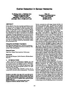
Fig. 1: Example of CD. Edge e12 has a larger CD than all edges in the cluster while its Euclidean distance is the same or smaller than their Euclidean distances. In this paper, we present a new method to find outliers using a measure called commute time distance, or commute distance for short (CD) 1 . CD is a well-known measure derived from a random walk on graph [11]. The CD between two nodes i and j in the graph is the number of steps that a random walk, starting from i will take to visit j and then come back to i for the first time. Indeed CD is a Mahalanobis distance in the space spanned by eigenvectors of the graph Laplacian matrix. Unlike traditional Mahalanobis distance, CD between two nodes can capture both the distance between them and their local neighborhood densities so that we can capture both global and local outliers using distance based methods such as methods in [2, 10]. Moreover, the method can be applied directly to graph data. To illustrate, consider a graph of five data points shown in Figure 1, which is built from a dataset of five observations. Denote dED (i, j) and dCD (i, j) as an Euclidean distance and a CD between observations i and j, respectively. The distances between all pairs of observations are in Table 1. Table 1: The Euclidean distance and CD for the graph in Figure 1. Euclidean Distance Index 1 2 3 4 1 0 1.00 1.85 1.85 2 1.00 0 1.00 1.00 3 1.85 1.00 0 1.41 4 1.85 1.00 1.41 0 5 2.41 1.41 1.00 1.00

5 2.41 1.41 1.00 1.00 0

Commute Distance 1 2 3 4 5 0 12.83 19.79 19.79 20.34 12.83 0 6.96 6.96 7.51 19.79 6.96 0 7.51 6.96 19.79 6.96 7.51 0 6.96 20.34 7.51 6.96 6.96 0

It can be seen that dCD (1, 2) is much larger than dCD (i, j) ((i, j) ∈ {2, 3, 4, 5}, i 6= j) even though dED (i, j) have the same or larger Euclidean distances than dED (1, 2). The CD from an observation outside the cluster to an observation inside the cluster is significantly larger than the CDs of observations inside the cluster. Since CD is a metric, a distance based method can be used to realize that point 1 is far away from other points using CD. Therefore, the use of CD is promising for identifying outliers. The contributions of this paper are as follows: – We prove that CD can naturally capture the local neighborhood density and establish a relationship between CD and local outlier detection. – We propose an outlier detection method using the CD metric to detect global and local outliers. The method can also detect outlying clusters which traditional methods often fail to capture. Moreover, the method is shown to be more resistant to noise than other local outlier detection methods. 1

A preliminary version of this work appeared as a technical report [8].

– We accelerate the computation of CD using a graph component sampling and an eigenspace approximation to avoid O(n3 ) computation. Furthermore, pruning technique is used to calculate the CD ‘on demand’. All of them speed up the method significantly to O(nlogn) while preserving the outlier ranking. The remainder of the paper is organized as follows. Section 2 reviews the theory of random walk on graph and CD. In Section 3, we introduce the method to detect outliers with the CD measure. Section 4 presents a way to approximate CD and accelerate the algorithm. In Section 5, we evaluate our approach using experiments on real and synthetic datasets. Section 6 is the conclusion.

2 2.1

Background Random Walk on Graph and Stationary Distribution

The random walk on a graph is a sequence of nodes described by a finite Markov chain which is time-reversible [11]. The probability that the random walk on node i at time t selects node j at time t + 1 is determined by the edge P weight on the graph: pij = P (s(t + 1) = j|s(t) = i) = wij /dii where dii = j∈adj(i) wij and adj(i) is a set of neighbors of node i. Let P be the transition matrix with entry pij , A is the graph adjacency matrix, and D is the diagonal matrix with entries dii . Then P = D−1 A. Denote πi (t) as the probability of reaching node i at time t, π(t) = [π1 (t), π2 (t), ..., πn (t)]T as the state probability distribution at time t, the state on transforming is π(t + 1) = P T π(t) and thus π(t) = (P T )t π(0) where π(0) is an initial state distribution. The distribution π(t) is stationary if π(t) = π(0) for all t > 0. 2.2

Commute Distance

This section reviews two measures of a random walk called hitting time h(i, j) and commute time c(i, j) [11]. The hitting time h(i, j) is the expected number of steps a random walk starting at i will take to reach j for the first time: ( 0 if i = j P h(i, j) = (1) 1 + k∈adj(i) pik h(k, j) otherwise. The commute time, which is known to be a metric and that is the reason for the term ‘commute distance’ [6], is the expected number of steps that a random walk starting at i will take to reach j once and go back to i for the first time: c(i, j) = h(i, j) + h(j, i).

(2)

The CD can be computed from the Moore-Penrose pseudoinverse of the graph Laplacian matrix [9, 6]. Denote L = D−A and L+ as the graph Laplacian matrix and its pseudoinverse respectively, the CD is: + + + c(i, j) = VG (lii + ljj − 2lij ),

(3)

Pn + where VG = i=1 dii is the volume of the graph and lij is the (i, j) element of + L . Equation 3 can be written as c(i, j) = VG (ei − ej )T L+ (ei − ej ),

(4)

where ei is the i-th column of an (n × n) identity matrix I [15]. Consequently, c(i, j)1/2 is a distance in the Euclidean space spanned by the ei ’s.

3 3.1

Commute Distance Based Outlier Detection A Proof of Commute Distance Property for Outlier Detection

We now show that CD is a good metric for local outlier detection. Lemma 1. The expected number of steps that a random walk which has just visited node i will take before returning back to i is VG /dii . Proof. For the proof of this Lemma, see [11]. Theorem 1. Given a cluster C and a point s outside C connected to a point t on the boundary of C (Fig. 2a). If C becomes denser (by adding more points or edges), the CD between s and t increases. Proof. From Lemma 1, the expected number of steps that a random walk which has just visited node s will take before returning back to s is VG /dss = VG /wst . Since the random walk can only move from s to t, VG /wst = h(s, t) + h(t, s) = c(s, t) (Fig. 2b). If cluster C becomes denser, there are more edges in cluster C. As a result, VG increases while wst is unchanged. So the CD between s and t (i.e c(s, t)) increases. u t As shown in Theorem 1, the denser the cluster, the larger the CD between a point s outside the cluster to a point t in the cluster. That is the reason why we can effectively detect local outliers using CD. 3.2

Outlier Detection Using Commute Distance

This section introduces a method based on CD to detect outliers. As CD is a metric and captures both the distance between nodes and their local neighborhood densities, we can use a CD based method to find global and local outliers. First, a mutual k1 -nearest neighbor graph is constructed from the dataset. The mutual k1 -nearest neighbor graph connects nodes u and v if u belongs to the k1 nearest neighbors of v and v belongs to the k1 nearest neighbors of u. The reason for choosing mutual k1 -nearest neighbor graph is that this graph tends to connect nodes within cluster of similar densities, but does not connect nodes from clusters of different densities [12]. Therefore, outliers are isolated and data clusters form graph components in mutual k1 -nearest neighbor graph. Moreover, the mutual k1 -nearest neighbor graph with n nodes (k1 ¿ n) is usually sparse,

s

t

(a)

(b)

Fig. 2: The CD from an outlier to an observation in a cluster increases when the cluster is denser. which has an advantage in computation. If the data has coordinates, we can use kd-tree to avoid O(n2 ) searching of nearest neighbors. The edge weights are inversely proportional to their Euclidean distances. However, it is possible that the mutual k1 -nearest neighbor graph is not connected so that we cannot apply random walk on the whole graph. One approach to make the graph connected is to find its minimum spanning tree and add the edges of the tree to the graph. Then the graph Laplacian matrix L and its pseudoinverse L+ are computed. After that the pairwise CDs between any two observations are calculated from L+ . Finally, the distance based outlier detection using CD with pruning technique proposed by Bay and Schwabacher [2] is used to find the top N outliers. The main idea of pruning is that an observation is not an outlier if its average distance to k2 current nearest neighbors is less than the score of the weakest outlier among top N found so far. Using this approach, a large number of non-outliers can be pruned without carrying out a full database scan. The outlier score used is the average distance of an observation to its k2 nearest neighbors. Suitable values for k1 (for building the nearest neighbor graph) and k2 (for estimating the outlier score) will be presented in the experiments.

4

Graph Component Sampling and Eigenspace Approximation

While CD is a robust measure for detecting both global and local outliers, its main drawback is its computational time. The direct computation of CD from L+ is proportional to O(n3 ) which is not feasible for large graphs (n is the number of nodes). In this work, the graph components are sampled to reduce the graph size and then eigenspace approximation in [15] is applied to approximate the CD on the sampled graph. 4.1

Graph Sampling

An easy way to sample a graph is selecting nodes from it uniformly at random. However, sampling in this way can break the graph geometry structure and outliers may not be chosen in sampling. To resolve this, we propose a sampling strategy called component sampling. After creating the mutual k1 -nearest neighbor graph, the graph tends to have many connected components corresponding to different data clusters. Outliers are either isolated nodes or nodes in very small components. For nodes in normal components (we have a threshold to distinguish between normal and outlying components), they are uniformly sampled

with the same ratio p = 50k1 /n, which is chosen from experimental results. For nodes in outlying components, we sample all of them. Then we rebuild a mutual k1 -nearest neighbor graph for the sampled data. Sampling in this way will maintain the geometry of the original graph and the relative densities of normal clusters. Outliers are also not sampled in this sampling strategy. 4.2

Eigenspace Approximation

Because the Laplacian matrix L (n×n) is symmetric and has rank n−1 [5], it can be decomposed as L = V SV T , where V is the matrix containing eigenvectors of L as columns and S is the diagonal matrix with the corresponding eigenvalues λ1 = 0 < λ2 < ... < λn on the diagonal. Then L+ = V S + V T where S + is the + + diagonal matrix with entries λ+ 1 = 1/λ2 > λ2 = 1/λ3 > ... > λn−1 = 1/λn > + T λn = 0. Equation 4 can be written as c(i, j) = VG (xi − xj ) (xi − xj ) where xi = S +1/2 V T ei [15]. Therefore, the CD between nodes on the graph can be viewed as the Euclidean distance in the space spanned by eigenvectors of the graph Laplacian matrix. Denote V˜ , S˜ as a matrix containing m largest eigenvectors of L+ and its corresponding diagonal matrix, and x ˜i = S˜+1/2 V˜ T ei , the approximate CD is c˜(i, j) = VG (˜ xi − x ˜j )T (˜ xi − x ˜j ),

(5)

The CD c(i, j) in an n dimensional space is transformed to the CD c˜(i, j) in an m dimensional space. Therefore, we just need to compute the m smallest eigenvectors with nonzero eigenvalues of L (i.e the largest eigenvectors of L+ ) to approximate the CD. This approximation is bounded by kc(i, j) − c˜(i, j)k ≤ Pm VG i=1 λ+ i [15]. 4.3

Algorithm

The proposed method is outlined in Algorithm 1. We create the sampled graph from the data using graph components sampling. Then the graph Laplacian L of the sampled graph and matrix V˜ (m smallest eigenvectors with nonzero eigenvalues of L) are computed. Since we use the pruning technique, we do not need to compute the approximate CD for all pairs of points. Instead, we compute Pm + it ‘on demand’ using the formula in equation 3 where ˜lij = k=1 λ+ k vik vjk , vjk and vjk are entries of matrix V˜ . 4.4

The Complexity of the Algorithm

The k-nearest neighbor graph with n nodes is built in O(nlogn) using kd-tree with the assumption that the dimensionality of the data is not very high. The average degree of each node is O(k) (k ¿ n). So the graph is sparse and thus finding connected components take O(kn). After sampling, the size of graph is O(ns ) (ns ¿ n). The standard method for eigen decomposition of L is O(n3s ). Since L is sparse, it would take O(N ns ) = O(kn2s ) where N is the number of

nonzeros. The computation of just the m smallest eigenvectors (m < ns ) is less expensive than that. The typical distance based outlier detection takes O(n2s ) for the neighborhood search. Pruning can scale it nearly linear. We only need to compute the CDs O(ns ) times each of which takes O(m). So the time needed for two steps is proportional to O(nlogn + kn + kn2s + mns ) = O(nlogn) as ns ¿ n. Algorithm 1 Commute Distance Based Outlier Detection with Graph Component Sampling and Eigenspace Approximation. Input: Data matrix X, the numbers of nearest neighbors k1 and k2 , the numbers of outliers to return N Output: Top N outliers 1: 2: 3: 4: 5: 6:

5

Construct the mutual k1 -nearest neighbor graph from the dataset Do the graph component sampling Reconstruct the mutual k1 -nearest neighbor graph from sampled data Compute the Laplacian matrix of the sampled graph and its m smallest eigenvectors Find top N outliers using the CD based technique with pruning rule (using k2 ) Return top N outliers

Experiments and Analysis

In this section, the effectiveness of CD as a measure for outlier detection is evaluated. Firstly, the ability of the distance based technique using CD (denoted as CDOF) in finding global, local outliers, and outlying clusters was tested in a synthetic dataset. The distance based technique using Euclidean distance [2] (denoted as EDOF) , LOF [3], and OutRank [13] (denoted as ROF and the same graph of CDOF was used) were also used to compare with CDOF. Secondly, the effectiveness of CDOF was evaluated in a real dataset. Thirdly, we have shown that CDOF is more resistant to small perturbations to data than LOF. Finally the performance and effectiveness of approximate CDOF were evaluated. The experiments were conducted on a workstation with an 3GHz Intel Core2 Duo processor and 2GB of main memory in Windows XP. 5.1

Synthetic Dataset

Figure 3a shows a 2-dimensional synthetic dataset. It contains one dense cluster of 500 observations (C1 ) and one sparse cluster of 100 observations (C2 ). Moreover, there are three small outlying clusters with 12 observations each (C3−5 ) and four outliers (O1−4 ). All the clusters were generated from a Normal distribution. O2 , O3 , O4 are global outliers which are far away from other clusters. O1 is a local outlier of dense cluster C1 . In the following experiments for this dataset, the numbers of nearest neighbors are k1 = 10 (for building the graph), k2 = 15 (for estimating the outlier score. Since the size of outlying clusters is twelve, fifteen is a reasonable number to estimate the outlier scores), and the number of top outliers is N = 40 (the

C

90

C

5

90

2

80

80 O

1

O2

70

70

C1

60

60 C3

O3

50

C4 50

40

40

O4

30

40

50

60

70

80

90

100

30

40

50

(a) Synthetic dataset

90

90

80

80

80

70

70

70

60

60

60

50

50

50

40

40

40

50

60

70

80

(c) EDOF

90

100

70

80

90

100

(b) CDOF

90

30

60

40

30

40

50

60

70

80

90

100

30

(d) LOF

40

50

60

70

80

90

100

(e) ROF

Fig. 3: Comparison of the results of EDOF, LOF, ROF, and CDOF. CDOF can detect all global, local outliers, and outlying clusters effectively. total observations in three outlying clusters and four outliers). The results are shown in Figure 3. The ‘x’ signs mark the top outliers found by each method. The figure shows that EDOF cannot detect local outlier O1 . Both EDOF and LOF cannot find two outlying cluster C3 and C4 . The reason is those two clusters are near each other with similar densities and consequently for each point in the two clusters the average distance to its nearest neighbors is small and the relative density is similar to that of its neighbors. Moreover, ROF outlier score is actually the node probability distribution when the random walk is stationary [13]. Therefore, it is dii /VG [11], which is small for outliers 2 . Therefore, it cannot capture nodes in the outlying clusters where dii is large. For degree one outlying nodes, ROF and CDOF have similar scores. The result in Figure 3b shows that CDOF can identify all the outliers and outlying clusters. The key point is in CD, inter-cluster distance is significantly larger then intra-cluster distance even if the two clusters are near in the Euclidean distance. 5.2

Real Dataset

In this experiment, CDOF was used to find outliers in an NBA dataset. The dataset contains information of all the players in the famous basketball league in the US in year 1997-1998. There were 547 players and six attributes were used: position, points per game, rebounds per game, assists per game, steals 2

This score has not been explicitly stated in the ROF paper.

per game and blocks per game. Point and assist reflect the offensive ability of a player while steal and block show how good a player is in defending. Rebound can be either offensive or defensive but total rebound is usually an indicator of defensive ability. The results are shown in Table 2 with the ranking and statistics of top five outliers. The table also shows the maximums, averages, and standard deviations for each attribute over all players. Table 2: The outlying NBA players. Rank 1 2 3 4 5

Player Dikembe Mutombo Dennis Rodman Michael Jordan Shaquille O’neal Jayson Williams Max Average Standard deviation

Position Center Forward Guard Center Forward

Points Rebounds Assists Steals Blocks 13.43 11.37 1.00 0.41 3.38 4.69 15.01 2.88 0.59 0.23 28.74 5.79 3.45 1.72 0.55 28.32 11.35 2.37 0.65 2.40 12.88 13.58 1.03 0.69 0.75 28.74 15.01 10.54 2.59 3.65 7.69 3.39 1.78 0.70 0.40 5.65 2.55 1.77 0.48 0.53

Dikembe Mutombo was ranked as the top outlier. He had the second highest blocks (5.6 times of standard deviation away from mean), the highest rebounds for center players, and high points. It is rare to have good scores in three or more different statistics and he was one of the most productive players. Dennis Rodman and Michael Jordan took the second and third positions because of their highest scores in rebound and point (4.6 and 3.7 times of standard deviation away from mean, respectively). Dennis Rodman was a rare case because his points were quite low among high rebound players as well. The next was Shaquille O’Neal who had the second highest points and high rebounds. He was actually the best scoring center and is likely a local outlier among center players. Finally, Jayson Williams had the second highest rebounds. It is interesting to note that except for Dennis Rodman because of his bad behaviour in the league, the other four players were listed in that year as members of All-Stars team [1]. 5.3

Sensitivity to Data Perturbation

In this section LOF and CDOF were compared on their ability to handle ‘noise’ perturbations in data. Recall that LOF (p) is the ratio between the average relative density of the nearest neighbors q of p over the relative density of p. LOF (p) is high (i.e p is outlier) if p’s neighborhood area is sparse and q’s neighborhood area is dense. Suppose that noise is uniformly distributed in the data space, it is obvious that the noise will have more effect on outliers than points in clusters. The noise data can be neighbors of outliers and their neighborhood are also sparse. Thus the numerator in LOF (p) formula where p is outlier reduces considerably while the denominator increases. As a result, LOFs of outliers may reduce significantly but they does not change much for points inside the clusters. Therefore, the relative rankings of data may not be preserved. On the other hand, uniform noise changes the nearest neighbor graph for CDOF in the way that degrees of outliers will increase but are still much smaller than degree of

4

3

x 10

100 EDOF LOF CDOF

2.5

800

90

700

80

1

F O

50

400

40

Time (s)

500

60

D

Time (s)

1.5

70

C

Outlier Percentage (%)

600 2

300

30 200 20

0.5

100

10 0

1

1.5

2

2.5

3 Data sizes

3.5

4

4.5

5

0

aCDOF 1000

4

x 10

2000

3000 Data Sizes

4000

5000

0

(a) Performances of EDOF, LOF, and ap- (b) Effectiveness of approximate CDOF proximate CDOF

Fig. 4: Performances of the method using approximate commute distance. points inside the clusters. Thus there will still be a big difference between intercluster and intra-cluster CDs. That maintains the higher scores for outliers than the points inside the cluster. To show this, we randomly added 10% noise from a uniform distribution to the synthetic dataset in Section 5.1 and applied LOF and CDOF in the new dataset. Then noise data was removed from the ranking. Two criteria were used to compare two methods: Spearman rank test for the ranking of the whole dataset and the similarity between the sets of top outliers before and after adding noise. The results were averaged over ten trials. Spearman rank test in LOF was 0.01 while the it was 0.48 for CDOF. It shows the relative ranking by LOF changes significantly due to noise effect. After adding noise, there were 62% of the original outliers still in the top outlier list for LOF while it was 92% for CDOF. CDOF is less sensitive as it combines local and global views of the data. Since noise is a kind of outlier, we cannot distinguish between outliers and noise but the preliminary results for noise effect show that the proposed method is more resistance to noise than the local outlier detection method. 5.4

Performances of the Proposed Method

In the following experiments, we compared the performances of EDOF, LOF, and approximate CDOF mentioned in Section 4. The experiment was performed using five synthetic datasets, each of which contained different clusters generated from Normal distributions and a number of random points. The number of clusters, the sizes, and the locations of the clusters were also chosen randomly. The results are shown in Figure 4a where the horizontal axis represents the dataset sizes in the ascending order and the vertical axis is the corresponding computational time. The result of approximate CDOF was averaged over ten trials of data sampling. It is shown that approximate CDOF is faster than LOF and slower than EDOF. This reflects the complexities of O(n), O(nlogn), and O(n2 ) for EDOF, approximate CDOF, and LOF, respectively. In order to validate the effectiveness of approximate CD, we used CD and approximate CD to find outliers in five synthetic datasets generated in the same

way as the experiment noted above with smaller sizes due to the high computation of CDOF. The results were averaged over ten trials. The results in Figure 4b shows approximate CDOF (aCDOF) is much faster than CDOF but still preserves a high percentage (86.2% on average) of top outliers found by CDOF. 5.5

Impact of Parameter k

In this section, we investigate how the number of nearest neighbors affects CDOF. Denote kmin as the maximum number of nodes that a cluster is an outlying cluster and kmax as the minimum number of nodes that a cluster is a normal cluster. There are two situations. If we choose the number of nearest neighbors k2 < kmin , nodes in an outlying cluster do not have neighbors outside the cluster. As a result, their outlier factors are small and we will miss them as outliers. On the other hand, if we choose k2 > kmax , nodes in a normal cluster have neighbors outside the cluster. And it is possible that some nodes in the cluster will be falsely recognized as outliers. The value of kmin and kmax can be considered as the lower and upper bounds for the number of nearest neighbors. They can be different depending on the application domains. In the experiment in Section 5.1, we chose k2 = 15, which is just greater than the sizes of all outlying clusters (i.e 12) and is less than the size of the smallest normal cluster (i.e 100). The same result can be obtained with 15 < k2 < 100 but it requires longer computational time. k2 is also chosen as a threshold to distinguish between normal and outlying clusters. Note that k2 mentioned in this section is the number of nearest neighbors for estimating the outlier scores. For building mutual k1 -nearest neighbor graph, if k1 is too small, the graph is very sparse and may not represent the dataset densities properly. In the experiment in Section 5.1, if k1 = 5, the algorithm misclassifies some nodes in the smaller normal cluster as outliers. If k1 is too large, the graph tend to connect together clusters whose sizes are less than k1 and are close to each other. Then some outlying clusters may not be detected if they connect to each other and form a normal cluster. k1 = 10 is found suitable for many synthetic and real datasets.

6

Conclusions

We have proposed a method for outlier detection using ‘commute distance’ as a metric to capture global, local outliers, and outlying clusters. The CD captures both distances between observations and their local neighborhood densities. We observed and proved a property of CD which is useful in capturing local neighborhood density. The experiments have shown the effectiveness of the proposed method in both synthetic and real datasets. Moreover, graph component sampling and eigenspace approximation used to approximate CD and the use of pruning rule can accelerate the algorithm significantly while still maintaining the accuracy of the detection. Furthermore preliminary experiments suggest that CDOF is less sensitive to perturbations in data than other measures.

7

Acknowledgement

The authors of this paper acknowledge the financial support of the Capital Markets CRC.

References 1. Database basketball. http://www.databasebasketball.com 2. Bay, S.D., Schwabacher, M.: Mining distance-based outliers in near linear time with randomization and a simple pruning rule. In: KDD ’03: Proc. of the ninth ACM SIGKDD international conference on Knowledge discovery and data mining. pp. 29–38. ACM, New York, NY, USA (2003) 3. Breunig, M.M., Kriegel, H.P., Ng, R.T., Sander, J.: Lof: Identifying density-based local outliers. In: Chen, W., Naughton, J.F., Bernstein, P.A. (eds.) Proc. of the 2000 ACM SIGMOD International Conference on Management of Data, May 1618, 2000, Dallas, Texas, USA. pp. 93–104. ACM (2000) 4. Chandola, V., Banerjee, A., Kumar, V.: Outlier detection: A survey. Tech. Rep. TR 07-017, Department of Computer Science and Engineering, University of Minnesota, Twin Cities (2007) 5. Chung, F.: Spectral Graph Theory. CBMS Regional Conference Series. No. 92, Conference Board of the Mathematical Sciences, Washington (1997) 6. Fouss, F., Renders, J.M.: Random-walk computation of similarities between nodes of a graph with application to collaborative recommendation. IEEE Transaction on Knowledge and Data Engineering 19(3), 355–369 (2007) 7. Hawkins, D.: Identification of Outliers. Chapman and Hall, London (1980) 8. Khoa, N.L.D., Chawla, S.: Unifying global and local outlier detection using commute time distance. Tech. Rep. 638, School of IT, University of Sydney (2009) 9. Klein, D.J., Randic, M.: Resistance distance. Journal of Mathematical Chemistry 12, 81–95 (1993), http://dx.doi.org/10.1007/BF01164627 10. Knorr, E.M., Ng, R.T.: Algorithms for mining distance-based outliers in large datasets. In: The 24rd International Conference on Very Large Data Bases. pp. 392–403 (1998) 11. Lov´ asz, L.: Random walks on graphs: a survey. Combinatorics, Paul Erd¨ os is Eighty 2, 1–46 (1993) 12. Luxburg, U.: A tutorial on spectral clustering. Statistics and Computing 17(4), 395–416 (2007) 13. Moonesinghe, H.D.K., Tan, P.N.: Outrank: a graph-based outlier detection framework using random walk. International Journal on Artificial Intelligence Tools 17(1), 19–36 (2008) 14. Rousseeuw, P.J., Leroy, A.M.: Robust Regression and Outlier Detection. John Wiley and Sons (2003) 15. Saerens, M., Fouss, F., Yen, L., Dupont, P.: The principal components analysis of a graph, and its relationships to spectral clustering. In: Proc. of the 15th European Conference on Machine Learning (ECML 2004). pp. 371–383. Springer-Verlag (2004) 16. Sun, P.: Outlier Detection In High Dimensional, Spatial And Sequential Data Sets. Ph.D. thesis, The University of Sydney (2006)