PAC Reinforcement Learning with an Imperfect Model Nan Jiang Microsoft Research, NYC
Motivation: sim2real transfer for RL
Sufficient conditions and algorithms
● Empirical success of deep RL (Atari games, MuJoCo, Go, etc.) ● Popular algorithms are sample-intensive for real-world applications
Definition 1: A partially corrected model MX is one whose dynamics are the same as M on X, and the same as M otherwise.
● Sim2real approach: (1) train in a simulator, (2) transfer to real world
Condition 1: V*(s0) is always higher in MX than in M for all X ⊆ Xξ-inc.
● Hope: reduce sample complexity with a high-fidelity simulator Compute policy
Collect data
(see the agnostic version of the conditions in the paper.) Theorem 1: Under Condition 1, there exists an algorithm that achieves O(|Xξ-inc|2 H4 log(1/δ)/ε3) sample complexity for ξ = O(ε/H2). Algorithm 1: illustration on previous example, Model 3.
Verify
Calibrate Simulator
Real environment
Figures from [1]
A simple theoretical question: If the simulator is only wrong in a small number of state-action pairs, can we substantially reduce #real trajectories needed?
● Collect data using optimal policy in simulator. ● Blue cells: plug in estimated dynamics along states w/ enough samples. Key steps in analysis: ● Accurate estimation of transition may require O(|S|) samples per (s, a). ● Incur dependence on |S|… need to avoid. ● Workaround: union bound over V* of all partially corrected models, which only incurs log(2|Xξ-inc|).
Answer: No! Further conditions are needed… Deeper thoughts: many scenarios in sim2real transfer ● What to transfer: policy, features, skills, etc. (we focus on policy)
What if we cannot change the model?
● How to quantify fidelity
Basic idea: ● Identify the wrong states as necessary. ● Terminate a simulated episode when running into wrong (s, a). = penalize a wrong (s, a) by fixing Q(s, a) = 0 (Vmin) in planning.
○ Prior theories (e.g., [2]) focus on global error (worst over all states) ○ Local errors (#states with large errors)? ● Is interactive protocol really better than non-interactive? Answer: Yes! (non-interactive: collect real data, calibrate the model, done)
Definition 2: A partially penalized model M\X is one that terminates on X, and have the same dynamics as M otherwise. Condition 2: V*(s0) is always higher in M\X than in M for all X ⊆ Xξ-inc.
Setup
Theorem 2: Under Condition 2, there exists an algorithm that achieves O(|Xξ-inc|2 H2 log(1/δ)/ε3) sample complexity for ξ = O(ε/H).
● Real environment: episodic MDP M = (S, A, P, R, H, s0).
Algorithm 2: M0 ← M , X0 ← {}. For t = 0, 1, 2, … ● Let πt be the optimal policy of Mt . Monte-Carlo evaluate πt.
● Simulator: M = (S, A, P , R, H, s0). ● Define Xξ-inc as the set of “wrong” (s, a) pairs where ● Goal: learn a policy π such that V*(s0) - Vπ(s0) ≤ ε, using only poly(|Xξ-inc|, H, 1/ε, 1/δ) real trajectories.
● Return if Vπt(s0) in M is close to V*(s0) in Mt. ● Sample real trajectories using πt . ● Once #samples from some (s, a) reaches threshold, compute
No dependence on |S| or |A; instead, adapt to the simulator’s quality. ● This is impossible without further assumptions...
● If large, Xt+1←Xt ∪ {(s, a)}, Mt+1←M\X .
Lower bound and hard instances
Non-interactive protocol is inefficient
● Lower bound: Ω(|S×A|/ε2), even when |X0-inc| = constant!
Theorem 3: “Collect data, calibrate, done” style algorithms cannot have poly(|Xξ-inc|, H, 1/ε, 1/δ) sample complexity, even with Conditions 1 & 2.
t+1
● Proof sketch: ○ Bandit hard instance: M = all arms Ber(½), except one w/ Ber(½+ ε)
Proof sketch: assume such an algorithm exists. Then,
○ Approximate model: M = all arms Ber(½) --- |X0-inc|=1 but useless
● The same dataset can calibrate multiple models.
● Illustration:
● Consider the hard instance in bandit. Design |A|2 models: ∀ a, a’∈ A, Ma, a’ = all arms Ber(½), except a & a’ w/ Ber(½+ ε). ● When a = a*, both Conditions 1 & 2 are met and |X0-inc| = 1.
Real environment
Model 1 (hard instance)
Model 2 (hard instance)
Model 3 (good cases)
○ Issue with Model 1: too pessimistic ○ Issue with Model 2: initially optimistic; pessimistic once error fixed ○ Good property of Model 3: always optimistic
● Hypothetical algorithm prefers a* to a’ with ⅔ prob. using a dataset of constant size. ● Majority vote from O(log|A|) datasets: boost success prob. to 1 - O(1/|A|). ● Solve bandit hard instance w/ polylog(|A|), against Ω(|A|) lower bound.
[1] Rusu et al. Sim-to-real robot learning from pixels with progressive nets. CoRL 2017. [2] Cutler et al. 2015. Real-world reinforcement learning via multifidelity simulators. IEEE Transaction on Robotics, 2015.